| Issue |
A&A
Volume 540, April 2012
|
|
|---|---|---|
| Article Number | A42 | |
| Number of page(s) | 7 | |
| Section | Stellar structure and evolution | |
| DOI | https://doi.org/10.1051/0004-6361/201118303 | |
| Published online | 22 March 2012 | |
Rotten Egg nebula: the magnetic field of a binary evolved star
1 Argelander Institute für Astronomie, Universität Bonn, Auf dem Hügel 71, 53121 Bonn, Germany
e-mail: This email address is being protected from spambots. You need JavaScript enabled to view it.
; This email address is being protected from spambots. You need JavaScript enabled to view it.
2 Department of Earth and Space Sciences, Chalmers University of Technology, Onsala Space Observatory, 439 92 Onsala, Sweden
3 JBCA, School of Physics & Astronomy, Manchester University, M13 9PL, UK
4 Department of Astronomy, University of Illinois at Urbana-Champaign, 1002 West Green Street, Urbana, IL 61801, USA
5 National Center for Supercomputing Applications, University of Illinois at Urbana-Champaign, 605 East Springfield Avenue, Champaign, IL 61820, USA
6 Joint Institute for VLBI in Europe, PO Box 2, 7990 AA Dwingeloo, The Netherlands
7 Leiden Observatory, Leiden University, PO Box 9513, 2300 RA Leiden, The Netherlands
8 Observatorio Astronómico Nacional, C/Alfonso XII 3, 28014 Madrid, Spain
Received: 19 October 2011
Accepted: 14 January 2012
Abstract
Context. Most of the planetary nebulae (PNe) observed are not spherical. The loss of spherical symmetry occurs somewhere between the asymptotic giant branch (AGB) phase and the PNe phase. The cause of this change of morphology is not yet well understood, but magnetic fields are one of the possible agents. The origin of the magnetic field remains to be determined, and potentially requires the presence of a massive companion to the AGB star. Therefore, further detections of the magnetic field around evolved stars, and in particular those thought to be part of a binary system, are crucial to improve our understanding of the origin and role of magnetism during the late stages of stellar evolution. One such binary is the pre-PN OH231.8+4.2, around which a magnetic field has previously been detected in the OH maser region of the outer circumstellar envelope.
Aims. We aim to detect and infer the properties of the magnetic field of the pre-PN OH231.8+4.2 in the H2O maser region that probes the region close to the central star. This source is a confirmed binary with collimated outflows and an envelope containing several maser species.
Methods. In this work we observed the 61,6−52,3 H2O maser rotational transition to determine its linear and circular polarization. As a result of Zeeman splitting, the properties of the magnetic field can be derived from maser polarization analysis. The H2O maser emissions of OH231.8+4.2 are located within the inner regions of the source (at a few tens of AU).
Results. We detected 30 H2O maser features around OH231.8+4.2. The masers occur in two distinct regions that are moving apart with a velocity on the sky of 2.3 mas/year. Taking into account the inclination angle of the source with the line of sight, this corresponds to an average separation velocity of 21 km s-1. Based on the velocity gradient of the maser emission, the masers appear to be dragged along the direction of the nebula jet. Linear polarization is present in three of the features, and circular polarization is detected in the two brightest features. The circular polarization results imply a magnetic field strength of |B||| ~ 45 mG.
Conclusions. We confirm the presence of a magnetic field around OH231.8+4.2, and report the first measurements of its strength within a few tens of AU of the stellar pair. Assuming a toroidal magnetic field, this imples B ~ 2.5 G on the stellar surface. The morphology of the field is not yet determined, but the high scatter found in the directions of the linear polarization vectors could indicate that the masers occur near the tangent points of a toroidal field.
Key words: masers / polarization / magnetic fields / stars: AGB and post-AGB
© ESO, 2012
1. Introduction
During the final stages of their evolution, low and intermediate mass stars (0.8−8 M⊙) evolve from the asymptotic giant branch (AGB) phase to planetary nebulae (PNe). During this transition most of these objects lose their spherical symmetry. The process responsible for the change of morphology is, so far, not well understood. Bujarrabal et al. (2001) have shown that, in most cases, the radiation pressure does not have enough energy to drive the acceleration of the fast bipolar flows observed in pre-PNe (pPNe). Moreover, the mass ejection on a preferred axis requires an extra agent to collimate the flow. The possible mechanisms that could both provide the missing energy to drive the fast flows and that could collimate it on a preferred axis are: (i) a companion to the star (either a binary stellar companion or massive planet) and its tidal forces, (ii) disk interaction and (iii) magnetic fields – or a combination of these (Balick & Frank 2002; Frank et al. 2007; Nordhaus et al. 2007, and references therein).
From magneto-hydrodynamic (MHD) simulations, García-Segura et al. (1999) concluded that magnetic fields can indeed have a pronounced effect on shaping stars beyond the AGB stage and that, working together with rotation, they can produce collimated bipolar nebulae and jets. Since then, several other MHD simulations have been designed to investigate how magnetic fields can shape a pPN and, consequently, a PN (e.g., García-Segura et al. 2005; García-Díaz et al. 2008; Dennis et al. 2009).
Observations of the magnetic fields around evolved stars, however, are still rare. Most current magnetic field measurements are performed using Zeeman splitting (Zeeman 1897) of maser lines (e.g., Vlemmings et al. 2001, 2006). Each maser species requires different physical conditions to occur. Therefore, different masers originate in different locations of the studied object. The SiO masers are found close to the central star (CS), in regions with a temperature of ~1300 K. The OH masers are generally expected to occur further out, at a few hundred AU from the CS. For AGB stars, the H2O maser emission is expected to be intermediate between these two regions; but for a pPN/PN it can be found at a similar or greater radius than the OH maser emission (Cohen 1987; Reid & Menten 1997; Vlemmings & Diamond 2006).
In this work, we aim to investigate the polarization of the H2O maser emission toward the pPN OH231.8+4.2 (Rotten Egg Nebula; Calabash Nebula), and infer the properties of its magnetic field. Located at a distance of ~1540 pc (Choi et al. 2011, updated from private communication), the bipolar nebula OH231.8+4.2 contains a binary system in its core, where a Main Sequence type A star accompanies an evolved star - the Mira variable QX Pup (Sanchez Contreras et al. 2004). The SiO, H2O and OH maser emission toward the Rotten Egg Nebula have been observed several times before (e.g., Morris et al. 1982; Gómez & Rodríguez 2001; Sanchez Contreras et al. 2002; Desmurs et al. 2007; Etoka et al. 2008, 2009). These prior works have shown that the spatial distribution of both the SiO and OH maser emission lie perpendicular to the nebular symmetry axis, consistent with the presence of a torus around the equator of the central star. However, the H2O masers (located at only ~40 AU from the CS) do not follow the same pattern, and are instead located toward the bipolar structure. Few of the prior studies included polarization measurements. Sanchez Contreras et al. (2002) note that their SiO polarization maps are not reliable and Gómez & Rodríguez (2001) found no circular polarization in the OH maser emission. Etoka et al. (2008, 2009), however, found both circular and linear polarization in the OH masers, and conclude that a well-organized magnetic field seems to be flaring out in the same direction as the outflow.
This paper is structured as follows: Sect. 2 describes the observations, data reduction, and calibration, and Sect. 3 includes a presentation of the results. The results are discussed in Sect. 4 and the concluding analysis is presented in Sect. 5.
2. Observations and data reduction
The observations of the pPN OH231.8+4.2 were carried out on March 1st, 2009, using the NRAO1 Very Long Baseline Array (VLBA), under project code BV067A. We observed the H2O 61,6 − 52,3 rotational transition, at an adopted rest frequency of 22.235081 GHz. We used 2 baseband filters of 1 MHz bandwidth and, following the VLBA H2O observations of Desmurs et al. (2007, hereafter D07), the filters were centered at Vlsr 44.0 km s-1 and 26.0 km s-1 respectively. This was done in order to detect both the emission from the northern (NReg; ~30 mas from the CS) and southern regions (SReg; ~40 mas from the CS) of the source. The observations were centered on RA0(J2000) = 07h42m16.93 and Dec0(J2000) = −14°42′ . Both a lower and a higher spectral resolution correlation were performed. The former was undertaken in full polarization mode (to obtain all 4 Stokes correlations: RR, LL, RL and LR) over 128 channels, with a resulting nominal channel width of 0.104 km s-1. The latter correlation was performed in dual polarization mode (to obtain RR and LL) over 512 channels, with a resulting nominal channel width of 0.026 km s-1. The synthesized beam size was ~1.7 × 0.9 mas. The observations spanned 8 h, of which 4.7 h were spent on OH231.8+4.2.
For calibration purposes, we observed J0854+2006. This reference source was used to perform bandpass, phase and polarization calibration. We used the Astronomical Image Processing Software Package (AIPS) and followed the data reduction procedure documented by Kemball et al. (1995), and which has been successfully adopted by several authors (e.g., Vlemmings et al. 2001; Surcis et al. 2011).
Using the low resolution data, we created image cubes for the Stokes parameters I, Q, U and V. The noise level measured from these image cubes ranges between ~3 and ~5 mJy/beam in the emission free channels. From the Stokes Q and U images, we derived image cubes for the linear polarization intensity (P) and the linear polarization direction (also referred to as electric vector position angle, EVPA).
Using the high resolution data, we created image cubes for the Stokes parameters I and V. The noise level measured from these image cubes lay between ~6 and ~10 mJy/beam in the emission free channels. To estimate the polarization leakage and consequently the minimum believable fractional linear polarization we determined the Stokes Q and U limits for the brightest maser feature with no detected polarization. We conclude that, at 3σ, the minimum detected fractional polarization is ~0.1%, a value that is consistent with the self-calibration method used during the data reduction, described in further detail by Leppänen et al. (1995).
In our analysis we adopted a signal-to-noise ratio cutoff of four times the measured noise (4σ). We define a maser feature to be successfully detected when maser spots located at similar spatial positions (within the beam size) appear and survive the threshold cut in at least 3 consecutive channels. The position of the maser feature is then defined by the emission in the channel where the peak appears (see e.g. Richards et al. 2011).
3. Results
3.1. Masers location
We detected 30 maser features in total, 20 of them located in the NReg and the remaining 10 located in the SReg. In Fig. 1 we present four plots: 1a and 1b correspond to the NReg, and 1c and 1d to the SReg. Plots (a) and (c) show the distribution of all 252 maser spots that comprise the 30 maser features. The dashed vectors indicate the direction of the pPN jet. Plots (b) and (d) show the maser features, scaled by their flux densities (proportional to the size of the triangles), and color-coded according to their line-of-sight velocities. The black line segments, scaled in size by the degree of polarization, show the EVPA (see Sect. 3.2). The origin (0, 0) of all four plots is centered on the brightest feature we detected, located in the SReg.
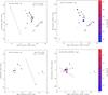 |
Fig. 1 Plots a) and b) (top) corresponds to NReg, and plots c) and d) (bottom) to SReg. Plots a) and c) (left) show the position of all the measured maser spots, and plots b) and d) (right) present the maser features. On plots a) and c) the dashed vectors indicate the direction of the pPN jet. On plots b) and d) the size of the triangles are scaled by the maser fluxes, and the color scale is related to the velocity. The black lines represent the EVPA and intensity of the linear polarization. |
In order to aid the comparison of the observations presented by D07 with the current work, we over-plotted both observations in Fig. 2. Since we did not use phase-referencing during our observations, unlike D07, we do not have a precise value for the absolute maser positions (but we do have accurate relative astrometric information). Therefore, to be able to make this comparison, we assumed a common origin point at the center of the maser emission. We determined this center point by taking the mean position over all the 30 maser features detected here, and over 15 of the 16 features detected by D07. We chose not to include maser feature number 16 from D07 in the analysis, because it is clearly a spatial outlier in the field that contains the features we observed. Figure 2 shows the entire field of view (NReg and SReg). The filled triangles represent the 30 features detected in the current work and the hollow squares show the observations from D07. Five regions (2.A, 2.B, 2.C, 2.D and 2.E) are drawn on the figure to facilitate their identification in the text.
In the NReg, the positions of the brightest feature and its surrounding features, are similar to those found by D07, except that the current observations detected more widespread features (region 2.A). On the eastern side of the brightest northern feature, at a separation of ~30 mas, we detected only one weak feature, while two features were detected by D07 in this region, at ~20 mas from the brightest maser (region 2.B). On the western side of the main feature we detected a group of 7 features that together seem to compose a single extended structure (region 2.C). This group of features does not appear in the observations of D07. Instead, they found only two features in that same region. Moreover, the emissions we detected in the NReg are contained within a much wider North-South area (~26 mas) than that in the D07 image (~13 mas).
In the SReg, the distribution of the features we observed is similar to those presented by D07, but appears to have moved away from the origin. Furthermore, we detected 10 features in this region, while D07 detected only six features (considering only regions 2.D and 2.E). The detections in the current observations are spread over a wider East-West area (~36 mas) than that reported by D07 (~17 mas).
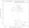 |
Fig. 2 Overplot of the maser features observed by D07 and the features presented in the present work. The filled triangles show the 30 features we observed and the hollow squares represent the observations from D07. The dashed vector indicate the direction of the pPN jet. |
The 30 maser features and their properties are listed in Table 1.
Maser features detected on OH231.8+4.2.
3.2. Linear polarization
We detected linear polarization for three of the 11 maser features in the SReg (S.05, S.06 and S.07). The degree of polarization and polarization angles of each feature are listed, with their respective errors, in Cols. 8 and 9 of Table 1. Those values correspond to the results given by the brightest channel of each feature. The P error is given by the rms taken from the P image, scaled by the intensity peak. The EVPA error was determined using the expression σEVPA = 0.5 σP/P × 180°/π (Wardle & Kronberg 1974).
In Fig. 1d, the black lines show the direction of the linear polarization of features S.05, S.06 and S.07. The length of the lines are proportional to the linear polarized intensity of each feature.
In Fig. 3, for each feature for which linear polarization was detected, we show the polarization vectors across all individual channels. Again the length of the vectors are scaled in proportion to the linearly-polarized intensity.
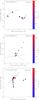 |
Fig. 3 Maser spots of the features S.05, S.06 and S.07. The triangle sizes are scaled to the intensity of each spot emission; the color scale shows how the velocity varies at each spot; and the black lines show the direction of linear polarization for those spots that have survived to the polarization threshold cut. The size of the black lines are scaled to the linearly-polarized intensity measured for each spot. |
3.3. Circular polarization
The total intensity (I) and circular polarization (V) spectra of the maser features were used to perform the Zeeman analysis described by Vlemmings et al. (2002). In this approach, the fraction of circular polarization, PV, is given by ![Mathematical equation: \begin{eqnarray} P_V &=& (V_{\rm max}~-~V_{\rm min})/I_{\rm max} \nonumber \\ &=& 2~\times A_{{\rm F}-{\rm F}'}~\times B_{||[{\rm Gauss}]} /\Delta v_{L[{\rm km\,s}^{-1}]} \end{eqnarray}](/articles/aa/full_html/2012/04/aa18303-11/aa18303-11-eq38.png) (1)where Vmax and Vmin are the maximum and minimum of the model fitted to the V spectrum and Imax is the peak flux of the emission. AF − F′ is the Zeeman splitting coefficient, whose exact value depends on the relative contribution of each hyperfine component of the H2O 61,6 − 52,3 rotational maser transition. We adopt the value AF − F′ = 0.018, which is the typical value reported by Vlemmings et al. (2002). B|| [Gauss] is the projected magnetic field strength along the line of sight, and ΔvL is the full- width half-maximum of the I spectrum. Although the non-LTE analysis in Vlemmings et al. (2002) has shown that the circular polarization spectra are not necessarily strictly proportional to dI/dν, using AF − F′ determined by a non-LTE fit introduces a fractional error of less than ~20% when using Eq. (1). To increase the signal-to-noise ratio of the I and V spectra, we smoothed the data by applying a running average over three consecutive channels. We note that the same result, albeit at lower signal-to-noise ratio, was obtained using the non-smoothed spectra.
(1)where Vmax and Vmin are the maximum and minimum of the model fitted to the V spectrum and Imax is the peak flux of the emission. AF − F′ is the Zeeman splitting coefficient, whose exact value depends on the relative contribution of each hyperfine component of the H2O 61,6 − 52,3 rotational maser transition. We adopt the value AF − F′ = 0.018, which is the typical value reported by Vlemmings et al. (2002). B|| [Gauss] is the projected magnetic field strength along the line of sight, and ΔvL is the full- width half-maximum of the I spectrum. Although the non-LTE analysis in Vlemmings et al. (2002) has shown that the circular polarization spectra are not necessarily strictly proportional to dI/dν, using AF − F′ determined by a non-LTE fit introduces a fractional error of less than ~20% when using Eq. (1). To increase the signal-to-noise ratio of the I and V spectra, we smoothed the data by applying a running average over three consecutive channels. We note that the same result, albeit at lower signal-to-noise ratio, was obtained using the non-smoothed spectra.
In Fig. 4 we show the spectra from Stokes I and V, with aI subtracted. Over-plotted on the V spectrum (red), we show the model curve that best fits the spectrum (blue). From this model fit, we derive a magnetic field strength of B||(NReg) = 44 ± 7 mG and B||(SReg) = −29 ± 21 mG. The reported errors are based on the single channel rms using Eq. (1), but similar errors were found using a chi-square analysis of the model circular polarization fitted to the smoothed spectra. We also further confirmed the result for both maser features by performing the chi-square analysis on spectra smoothed to different spectral resolutions (up to ~0.2 km s-1). This leads us to conclude that the detection in the SReg is marginally significant. The flux densities of the other 28 features, however, where not sufficient for a detection of circular polarization.
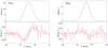 |
Fig. 4 Spectra of the Stokes I (top) and V (bottom). On the left hand side we present the spectra on the spatial position of the peak emission of the NReg. On the right hand side we show the spectra on the spatial position of the peak emission of the SReg. From the best fit model (blue line) we obtained B||(NReg) = 44 ± 7 mG and B||(SReg) = −29 ± 21 mG. |
4. Discussion
4.1. Kinematics
Assuming that the maser features observed in this work, at the epoch of March 1st 2009, correspond to approximately the same features detected by D07 on November 24th 2002, we can estimate the apparent proper motion between both observational epochs. We compared the distance between the mean position of all features located in region 2.A to the mean position of all features located in region 2.D in our data (Fig. 2), against the distance between the two corresponding points from D07. We present these mean positions and the offsets between the two observational epochs in Table 2. The offsets2 in α and δ give a total offset of 14.4 mas which, at a distance of 1540 pc, corresponds to 22.2 AU. Accordingly, for the time elapsed between the observations (2288 days), the velocity of the separation between the two mean points on the sky is computed to be 2.3 mas/year, or 16 km s-1. Assuming the inclination of the bipolar flow is i = 36° (Kastner et al. 1992; Shure et al. 1995), the real separation velocity is 21 ± 11 km s-1.
Furthermore, we considered the overall distribution of the maser spots for all features that we observed. In Fig. 1a we show that the spots in the NReg appear to align well with the direction of the nebular jet. The same property is found for the spots from the SReg, as can be seen more clearly in Fig. 3. In particular, the spots from feature S.07 appear to be closely aligned with the direction of the jet. However, despite being co-linear with the jet, the H2O maser outflow velocity is significantly lower than that reported for the jet, vjet ~ 330 km s-1 (Sanchez Contreras 1997). Hence, our interpretation is that the masers are being entrained by the jet but are not located in the jet itself. As a consequence, the maser spots have a velocity gradient; with higher velocity further from the origin. The nature of the H2O masers in OH231.8+4.2 is thus very different from that of the water fountain sources where the H2O masers lie at the tip of their fast bipolar outflows (e.g. Imai et al. 2002).
It is important to highlight, however, that a more precise kinematics analysis will require more accurate astrometric observations.
4.2. Polarization
We detected linear polarization for three H2O maser features, all of them located in the SReg (S.05, S.06 and S.07). According to maser polarization theory, the direction of the linear polarization can be either parallel or perpendicular to the direction of the magnetic field lines. It is parallel when the angle between the magnetic field and the direction of maser propagation (θ) is less than the van Vleck angle (~55°), and it is perpendicular when θ is greater than this angle (Goldreich 1973). The percentage of linear polarization is affected by θ and by the degree of saturation. Based on the level of linear polarization detected (~1%) we cannot conclude definitively in which regime – parallel or perpendicular – the masers of OH231.8+4.2 occur.
The linear polarization angles of the features S.05, S.06 and S.07 display a significant scatter (Fig. 1d). The cause of this scatter is not known, but we propose three different scenarios: (i) the scatter could be caused by turbulence, or (ii) in the case of a toroidal magnetic field, the masers could be located at its tangent points; both would explain the different local directions of the field, or (iii) the scatter could be caused by internal Faraday rotation (Faraday 1845). Under the effect of Faraday rotation, the linear polarization angle of the emission (Φ) is rotated by ![Mathematical equation: \begin{eqnarray} \Phi[^\circ]=2.02~\times 10^{-2}~L[{\rm AU}]~n_{\rm e}[{\rm cm}^{-3}]~B_{||}[m{\rm G}]~\nu^{-2}[{\rm GHz}] \end{eqnarray}](/articles/aa/full_html/2012/04/aa18303-11/aa18303-11-eq57.png) (2)where L is the path-length of the maser emission through a medium with magnetic field B|| and electron density ne at a frequency ν. By assuming typical values L ~ 10 AU and B|| ~ 50 mG for the H2O masers, Eq. (2) becomes: Φ ~ 0.02° × ne. For the Faraday rotation angle to be of the order of the observed scatter, an electron density of order 103 is required. For example, if ne ~ 2000 cm-3, then Φ ~ 40°. For an electron density of this order at this distance to the central star(s), the fractional ionization would be significantly higher then for a regular evolved star. However, considering the pre-PN nature of OH231.8+4.2 this cannot be completely ruled out. Still, we consider either scenarios (i) and (ii) more likely than the internal Faraday rotation effect. We note, however, that both scenarios (i) and (ii) differ from the results reported by Etoka et al. (2009) for the OH maser region. The OH masers indicate a uniform field that seems to be flaring out in the same direction of the jet. However, the H2O and OH masers occur in very different regions. While the current work finds the H2O masers to be located at ~40 AU from the CS, the OH masers are located on a torus with a radius of ~2 arcsec (Zijlstra et al. 2001; Etoka et al. 2008). At 1540 pc this correspond to a distance of ~ 3100 AU.
(2)where L is the path-length of the maser emission through a medium with magnetic field B|| and electron density ne at a frequency ν. By assuming typical values L ~ 10 AU and B|| ~ 50 mG for the H2O masers, Eq. (2) becomes: Φ ~ 0.02° × ne. For the Faraday rotation angle to be of the order of the observed scatter, an electron density of order 103 is required. For example, if ne ~ 2000 cm-3, then Φ ~ 40°. For an electron density of this order at this distance to the central star(s), the fractional ionization would be significantly higher then for a regular evolved star. However, considering the pre-PN nature of OH231.8+4.2 this cannot be completely ruled out. Still, we consider either scenarios (i) and (ii) more likely than the internal Faraday rotation effect. We note, however, that both scenarios (i) and (ii) differ from the results reported by Etoka et al. (2009) for the OH maser region. The OH masers indicate a uniform field that seems to be flaring out in the same direction of the jet. However, the H2O and OH masers occur in very different regions. While the current work finds the H2O masers to be located at ~40 AU from the CS, the OH masers are located on a torus with a radius of ~2 arcsec (Zijlstra et al. 2001; Etoka et al. 2008). At 1540 pc this correspond to a distance of ~ 3100 AU.
We detected circular polarization for two maser features. Based on these detections, we determined the strength of the magnetic field in each feature to be (B||(NReg) = 44 ± 7 mG, B||(SReg) = −29 ± 21 mG). If, as argued in Sect. 3.3 that the detection in the SReg is marginally significant, it is evident that the magnetic field in the SReg has an opposite sign compared to the field in the NReg – the positive sign indicates that the direction of the magnetic field is away from the observer, while the negative sign corresponds to a direction towards the observer.
A precise determination of the morphology of the magnetic field is not possible from the current work, as different field morphologies can fit the circular and linear polarization results obtained here. To reach a final conclusion as to the morphology of the magnetic field of OH231.8+4.2 more sensitive polarization information is necessary. If, however, we assume a toroidal3 magnetic field (B ∝ r-1), it is possible to extrapolate the field strength to the stellar surface. By taking the separation between the NReg and SReg, and assuming that the CS is located centrally between the two, each H2O maser region is at ~40 AU from the star. Therefore, from the measured B|| for these regions, the magnetic field strength on the stellar surface (taken to have a radius of ~1 AU) must be ~2.5 G.This is consistent with the result found for W43A (1.5 G; Vlemmings et al. 2006). This value presents a lower limit if the magnetic field vs. radius relation has a steeper than toroidal dependence.
5. Conclusions
We detected 30 H2O maser features towards OH231.8+4.2. By comparing the current work with the prior observations of Desmurs et al. (2007), we can conclude that the features are moving away from the central star. The average separation velocity of the masers is 21 ± 11 km s-1. Furthermore, the masers appear to be dragged in the direction of the collimated outflow. This likely indicates that the masers arise in the turbulent material that is entrained by the jet.
We detected linear polarization for three H2O maser features. The large scatter in the directions of the linear polarization could be caused by turbulence, or could be due to the masers being located close to the tangent points of a toroidal magnetic field. The possibility of Faraday rotation has also been investigated but, unless the electron density is exceptionally high ( ≳ 2000 cm-3), is ruled out.
Based on the detection of circular polarization for two maser features, we determined that the strength of the source magnetic field is B||(NReg) = 44 ± 7 mG and B||(SReg) = −29 ± 21 mG. The exact morphology of the field in the H2O maser region could however not be determined. Assuming a toroidal magnetic field (B ∝ r-1), the extrapolated magnetic field strength on the stellar surface is ~ 2.5 G.
Our polarization detections, together with the results from Etoka et al. (2009), make pPN OH231.8+4.2 the first evolved star that is known to be a binary and in which the presence of a magnetic field is confirmed throughout the circumstellar envelope. A more comprehensive model of the magnetic field morphology and its potential evolution based on a comparison of the inner and outer wind will require more sensitive observations.
The National Radio Astronomy Observatory (NRAO) is a facility of the National Science Foundation operated under cooperative agreement by Associated Universities, Inc.
These offsets occur in tangent plane project in the sky. So, strictly, the α and δ listed in Table 2 correspond to the coordinate angles of these projections.
Note that solar-type and dipole fields have r-2 and r-3 dependencies, respectively.
Acknowledgments
M.L.L.-F. would like to thank Dr. G. Surcis, Dr. R. Franco-Hernández and the anonymous referee for their useful suggestions, that helped to improved the paper. This research was supported by the Deutscher Akademischer Austausch Dienst (DAAD) and the Deutsche Forschungsgemeinschaft (DFG; through the Emmy Noether Research grant VL 61/3-1).
References
- Balick, B., & Frank, A., 2002, ARA&A, 40, 439 [NASA ADS] [CrossRef] [Google Scholar]
- Bujarrabal, V., Castro-Carrizo, A., Alcolea, J., & Sánchez Contreras, C. 2001, A&A, 377, 868 [NASA ADS] [CrossRef] [EDP Sciences] [Google Scholar]
- Choi, Y. K., Brunthaler, A., Menten, K. M., & Reid, M. J. 2011, IAUS, submitted [Google Scholar]
- Cohen, R. J. 1987, IAUS, 122, 229 [NASA ADS] [Google Scholar]
- Dennis, T. J., Frank, A., Blackman, E. G., et al. 2009, ApJ, 707, 1485 [NASA ADS] [CrossRef] [Google Scholar]
- Desmurs, J.-F., Alcolea, J., Bujarrabal, V., et al. 2007, A&A, 468, 189 [NASA ADS] [CrossRef] [EDP Sciences] [Google Scholar]
- Etoka, S., Lagadec, E., Zijlstra, A. A., et al. 2008, Proc. Sci., 63 [Google Scholar]
- Etoka, S., Zijlstra, A., Richards, A. M., Matsuura, M., & Lagadec, E. 2009, ASPC, 404, 311 [NASA ADS] [Google Scholar]
- Faraday, M. 1845, Faraday’s Diary of Experimental Investigation, IV [Google Scholar]
- Frank, A., De Marco, O., Blackman, E., & Balick, B. 2007, unpublished [arXiv:0712.2004] [Google Scholar]
- García-Díaz, M. T., López, J. A., Richer, M. G., & Steffen, W. 2008, ApJ, 676, 402 [NASA ADS] [CrossRef] [Google Scholar]
- García-Segura, G., Langer, N., Różyczka, M., & Franco, J. 1999, ApJ, 517, 767 [NASA ADS] [CrossRef] [Google Scholar]
- García-Segura, G., López, J. A., & Franco, J. 2005, ApJ, 618, 919 [NASA ADS] [CrossRef] [Google Scholar]
- Goldreich, P., Keeley, D. A., & Kwan, J. Y. 1973, ApJ, 179, 111 [NASA ADS] [CrossRef] [Google Scholar]
- Gómez, Y., & Rodríguez, L. F. 2001, ApJ, 557, 109 [Google Scholar]
- Imai, H., Obara, K., Diamond, P. J., Omodaka, T., & Sasao, T. 2002, Nature, 417, 829 [NASA ADS] [CrossRef] [PubMed] [Google Scholar]
- Kastner, J. H., Weintraub, D. A., Zuckerman, B., et al. 1992, ApJ, 398, 552 [NASA ADS] [CrossRef] [Google Scholar]
- Kemball, A. J., Diamond, P. J., & Cotton, W. D. 1995, A&AS, 110, 383 [NASA ADS] [Google Scholar]
- Leone, F., Martínez González, M. J., Corradi, R. L. M., Privitera, G., & Manso Sainz, R. 2011, ApJ, 731, 33 [Google Scholar]
- Leppänen, K. J., Zensus, J. A., & Diamond, P. J. 1995, AJ, 110, 2479 [NASA ADS] [CrossRef] [Google Scholar]
- Morris, M., Bowers, P. F., & Turner, B. E. 1982, ApJ, 259, 625 [Google Scholar]
- Nordhaus, J., Blackman, E. G., & Frank, A. 2007, MNRAS, 376, 599 [NASA ADS] [CrossRef] [Google Scholar]
- Reid, M. J., & Menten, K. M. 1997, ApJ, 476, 327 [NASA ADS] [CrossRef] [Google Scholar]
- Richards, A. M. S., Elitzur, M., & Yates, J. A. 2011, A&A, 525, A56 [NASA ADS] [CrossRef] [EDP Sciences] [Google Scholar]
- Sánchez Contreras, C. 1997, AcC, 23, 175 [NASA ADS] [Google Scholar]
- Sánchez Contreras, C., Desmurs, J. F., Bujarrabal, V., Alcolea, J., & Colomer, F. 2002, A&A, 385, 1 [Google Scholar]
- Sánchez Contreras, C., Gil de Paz, A., & Sahai, R. 2004, ApJ, 616, 519 [NASA ADS] [CrossRef] [Google Scholar]
- Shure, M., Sellgren, K., Jones, T. J., & Klebe, D. 1995, AJ, 109, 721 [NASA ADS] [CrossRef] [Google Scholar]
- Surcis, G., Vlemmings, W. H. T., Curiel, S., et al. 2011, A&A, 527, A48 [NASA ADS] [CrossRef] [EDP Sciences] [Google Scholar]
- Vlemmings, W. H. T., & Diamond, P. J. 2006, ApJ, 648, 59 [Google Scholar]
- Vlemmings, W., Diamond, P. J., & van Langevelde, H. J. 2001, A&A, 375, 1 [NASA ADS] [CrossRef] [EDP Sciences] [Google Scholar]
- Vlemmings, W. H. T., Diamond, P. J., & van Langevelde, H. J. 2002, A&A, 394, 589 [NASA ADS] [CrossRef] [EDP Sciences] [Google Scholar]
- Vlemmings, W. H. T., Diamond, P. J., & Imai, H. 2006, Nature, 440, 58 [NASA ADS] [CrossRef] [PubMed] [Google Scholar]
- Wardle, J. F. C., & Kronberg, P. P. 1974, ApJ, 194, 249 [NASA ADS] [CrossRef] [Google Scholar]
- Zeeman, P. 1897, Philos. Mag., 43, 226 [Google Scholar]
- Zijlstra, A. A., Chapman, J. M., te Lintel Hekkert, P., et al. 2001, MNRAS, 322, 280 [NASA ADS] [CrossRef] [Google Scholar]
All Tables
All Figures
|
Fig. 1 Plots a) and b) (top) corresponds to NReg, and plots c) and d) (bottom) to SReg. Plots a) and c) (left) show the position of all the measured maser spots, and plots b) and d) (right) present the maser features. On plots a) and c) the dashed vectors indicate the direction of the pPN jet. On plots b) and d) the size of the triangles are scaled by the maser fluxes, and the color scale is related to the velocity. The black lines represent the EVPA and intensity of the linear polarization. |
| In the text | |
|
Fig. 2 Overplot of the maser features observed by D07 and the features presented in the present work. The filled triangles show the 30 features we observed and the hollow squares represent the observations from D07. The dashed vector indicate the direction of the pPN jet. |
| In the text | |
|
Fig. 3 Maser spots of the features S.05, S.06 and S.07. The triangle sizes are scaled to the intensity of each spot emission; the color scale shows how the velocity varies at each spot; and the black lines show the direction of linear polarization for those spots that have survived to the polarization threshold cut. The size of the black lines are scaled to the linearly-polarized intensity measured for each spot. |
| In the text | |
|
Fig. 4 Spectra of the Stokes I (top) and V (bottom). On the left hand side we present the spectra on the spatial position of the peak emission of the NReg. On the right hand side we show the spectra on the spatial position of the peak emission of the SReg. From the best fit model (blue line) we obtained B||(NReg) = 44 ± 7 mG and B||(SReg) = −29 ± 21 mG. |
| In the text | |
Current usage metrics show cumulative count of Article Views (full-text article views including HTML views, PDF and ePub downloads, according to the available data) and Abstracts Views on Vision4Press platform.
Data correspond to usage on the plateform after 2015. The current usage metrics is available 48-96 hours after online publication and is updated daily on week days.
Initial download of the metrics may take a while.