| Issue |
A&A
Volume 540, April 2012
|
|
|---|---|---|
| Article Number | A57 | |
| Number of page(s) | 21 | |
| Section | Galactic structure, stellar clusters and populations | |
| DOI | https://doi.org/10.1051/0004-6361/201117637 | |
| Published online | 27 March 2012 | |
The present-day mass function of the Quintuplet cluster based on proper motion membership⋆,⋆⋆,⋆⋆⋆
1 Argelander Institut für Astronomie, Universität Bonn, Auf dem Hügel 71, 53121 Bonn, Germany
e-mail: This email address is being protected from spambots. You need JavaScript enabled to view it.
; This email address is being protected from spambots. You need JavaScript enabled to view it.
2 Max-Planck-Institut für Astronomie, Königsstuhl 17, 69117 Heidelberg, Germany
e-mail: This email address is being protected from spambots. You need JavaScript enabled to view it.
; This email address is being protected from spambots. You need JavaScript enabled to view it.
3 Max-Planck-Institut für Radioastronomie, Auf dem Hügel 69, 53121 Bonn, Germany
e-mail: This email address is being protected from spambots. You need JavaScript enabled to view it.
Received: 5 July 2011
Accepted: 14 February 2012
Abstract
Context. The stellar mass function is a probe for a potential dependence of star formation on the environment. Only a few young clusters are known to reside within the central molecular zone and can serve as testbeds for star formation under the extreme conditions in this region.
Aims. We determine the present-day mass function of the Quintuplet cluster, a young massive cluster in the vicinity of the Galactic centre.
Methods. We use two epochs of high resolution near infrared imaging data obtained with NAOS/CONICA at the ESO VLT to measure the individual proper motions of stars in the Quintuplet cluster in the cluster reference frame. An unbiased sample of cluster members within a radius of 0.5 pc from the cluster centre was established based on their common motion with respect to the field and a subsequent colour-cut. Initial stellar masses were inferred from four isochrones covering ages from 3 to 5 Myr and two sets of stellar evolution models. For each isochrone, the present-day mass function of stars was determined for the full sample of main sequence cluster members using an equal number binning scheme.
Results. We find the slope of the present-day mass function in the central part of the Quintuplet cluster to be α = -1.68+0.13-0.09 for an approximate mass range from 5 to 40 M⊙, which is significantly flatter than the Salpeter slope of α = −2.35. The flattening of the present-day mass function may be caused by rapid dynamical evolution of the cluster in the strong Galactic centre tidal field. The derived mass function slope is compared to the values found in other young massive clusters in the Galaxy.
Key words: Galaxy: center / open clusters and associations: individual: Quintuplet cluster / stars: early-type / infrared: stars / stars: luminosity function, mass function / stars: kinematics and dynamics
Based on observations collected at the ESO/VLT under Program ID 71.C-0344(A) (PI: F. Eisenhauer, retrieved from the ESO archive) and Program ID 081.D-0572(B) (PI: W. Brandner).
Appendices are available in electronic form at http://www.aanda.org
Full Table 4 is available at the CDS via anonymous ftp to cdsarc.u-strasbg.fr (130.79.128.5) or via http://cdsarc.u-strasbg.fr/viz-bin/qcat?J/A+A/540/A57
Member of the International Max Planck Research School for Astronomy and Cosmic Physics at the University of Heidelberg, IMPRS-HD, Germany.
© ESO, 2012
1. Introduction
The Quintuplet cluster is one of only three young massive clusters known within the central molecular zone (CMZ) with projected distances of less than 30 pc to Sagittarius A∗, the supermassive black hole (SMBH) at the centre of the Milky Way. The other two clusters are the Arches cluster at a similar location as the Quintuplet cluster, and the nuclear star cluster surrounding Sgr A∗. These clusters are unique laboratories to study the formation and evolution of stars and their host clusters in the Galactic centre (GC) environment.
The conditions for star formation in the CMZ and the GC region are rather extreme in terms of high gas densities, enhanced temperatures, tidal forces exerted by the gravitational potential in the inner Galaxy, and strong magnetic fields. These conditions were suggested to favour the formation of high mass stars as compared to the more moderate spiral arm environments (Morris 1993; Morris & Serabyn 1996). An overpopulation of high mass stars may be evidenced in a flattened initial mass function (IMF) in GC star clusters. The young massive clusters are ideal candidates to search for such a deviation from the Galactic field IMF. Their youth ensures that a large fraction of the initial population is still present in or near the cluster and their high total masses provide coverage of the entire mass function (MF) up to the highest-mass stars known, such as the Pistol star in the Quintuplet cluster (Figer et al. 1995; Figer et al. 1998; Yungelson et al. 2008). Due to the large number of high mass stars these cluster are also well-suited to assess stellar evolution scenarios for the most massive stars.
A direct comparison of the observed present-day mass function (PDMF) of the GC young massive clusters with the Galactic field IMF is aggravated due to their rapid dynamical evolution and dissolution in the GC tidal field. N-body simulations of compact massive clusters with masses ≤2 × 10⁴ M⊙ and distances from the GC ≤ 100 pc by Kim et al. (2000) yielded dissolution times of less than 10 Myr. A similar study by Portegies Zwart et al. (2002) derived somewhat longer dissolution times of up to 55 Myr for a GC distance of 150 pc, but found that the spatial density of a young massive cluster drops quickly below the background density within a few Myr, rendering older clusters indetectable.
In spite of this difficulty, measuring the PDMF is essential to deduce the IMF and to compare star formation in the GC with the outcome in less extreme environments. As the cluster centre is least affected by tidal stripping, as opposed to the outer cluster areas, the slope of the PDMF there can be compared to the PDMF slopes of spiral arm young massive clusters. In addition, tidally stripped stars might still be located close to the cluster at these young ages. If these stars can be identified as former cluster members, e.g. as they are co-moving with the cluster at comparable velocities, the common PDMF of cluster members and former members might still be a reasonable representation of the IMF. Most notably the measured PDMF of a GC cluster is an indispensable ingredient to constrain dynamical simulations set out to reconstruct its dynamical history, its IMF and to recover possible IMF variations.
The name of the Quintuplet cluster arises from a “quintuplet” of bright near-infrared (NIR) sources (Q1–Q4, Q9), which was first observed by Nagata et al. (1990) and Okuda et al. (1990) by resolving one or two merged sources present in earlier surveys (e.g. Kobayashi et al. 1983). Shortly afterwards, the number of resolved cluster stars was increased to 15 stars (Q1–Q15, Glass et al. 1990; the “Q”-label was introduced in Figer et al. 1999b). Until today, 21 Wolf-Rayet (WR) stars (14 WC, 7 WN stars, see van der Hucht 2006, and references therein; Mauerhan et al. 2010b; Liermann et al. 2009, 2010), two luminous blue variables (LBVs) and 93 OB stars were spectroscopically identified (Figer et al. 1999b; Liermann et al. 2009). Hence, the Quintuplet hosts almost a quarter of the 92 WR stars in the Galactic centre region (Mauerhan et al. 2010a). The age of the cluster was derived based on spectral types of likely cluster stars to be 4 ± 1 Myr (Figer et al. 1999b). The Quintuplet cluster is therefore slightly older than the Arches cluster (age: 2−2.5 Myr, Najarro et al. 2004), with whom it shares a similar projected GC distance (30 pc and 26 pc, respectively), a similar location in the sky and comparable masses of the order of 104 M⊙. As the density of the Quintuplet cluster is more than two orders of magnitude lower than the density of the Arches cluster (Figer 2008), and it exhibits a much more dispersed appearance, it is suggestive to regard these two clusters as snapshots at different timesteps of massive clusters rapidly dissolving in the GC tidal field.
Due to the strong interstellar extinction for lines of sight towards the GC and the large distance to these clusters, NIR observations with high spatial resolution provided either by ground based telescopes with AO correction or space telescopes are required to study their stellar populations. As the Quintuplet cluster is far less compact than the Arches cluster, it is mandatory even in the cluster core to apply an effective method to discern the cluster stars from field stars in order to determine cluster properties in an unbiased way. In this paper, we analyse adaptive optics (AO) observations of the Quintuplet cluster obtained with the NAOS-CONICA (NACO) instrument on the ESO Very Large Telescope (VLT). A clean sample of cluster stars was established based on the measurement of individual proper motions and a subsequent colour-cut. The determination of proper motion membership allowed us to derive the PDMF of the central part of the Quintuplet cluster for the first time.
In Sect. 2 we present the data and the data reduction. The source extraction, the photometric calibration and the determination of the astrometric and photometric uncertainties are detailed in Sect. 3. The completeness of detected stars is derived from artificial star experiments in Sect. 4. The proper motion of individual stars is determined in Sect. 5, and the proper motion membership sample is established. The colour-magnitude diagrams (CMDs) of proper motion members and non-members are discussed in Sect. 6, and the final cluster sample is derived applying a colour-cut and using spectral identifications from the spectral catalogue by Liermann et al. (2009). Initial stellar masses are determined in Sect. 7 from four isochrones of different ages and different stellar models. The arising PDMFs of the four isochrones are discussed in Sect. 8. In Sect. 9, we compare our results to reported mass function slopes of other young massive clusters in the Milky Way. This paper concludes with a short summary in Sect. 10.
Overview of the VLT/NAOS-CONICA datasets.
2. Observations and data reduction
Two epochs of high-resolution observations of the Quintuplet Cluster (α = 17h46m15s, δ = −28°49′41″, J2000) were obtained in service mode on July 22–23th 2003 and July 24th 2008 with the VLT, yielding a time baseline of 5.0 yr. In order to achieve the high astrometric accuracy crucial for this study, the near-infrared imaging camera CONICA was used in combination with the NAOS instrument providing AO correction (Lenzen et al. 2003; Rousset et al. 2003). The first epoch was observed with a Santa Barbara Research Center (SBRC) InSb Aladdin2 array detector, which was replaced by an InSb Aladdin3 array in May 2004 (Ageorges et al. 2007). All data were taken with the medium-resolution camera (S27) with a pixel scale of 0.0271″ pixel-1 and a field of view of 27.8″. The Quintuplet star Q2 (Glass et al. 1990) with Ks ~ 6.6 mag served as the natural guide star for the infrared wavefront sensor. The data of the first epoch was retrieved from the ESO archive (PI: F. Eisenhauer, Program ID 71.C-0344(A)) and consisted of three datasets: two datasets in the H- and Ks-band with a short detector integration time (DIT) of 2.0 s and a further Ks-band dataset with a longer DIT of 20.0 s to expand the range of observed magnitudes towards fainter stars. Each of these three datasets map an effective field of view of about 40″ × 40″. The Ks-band observations of the second epoch in 2008 cover the same field of view as the first epoch. The details of all four datasets such as the number of integrated DITs (NDIT) and the total exposure time are summarized in Table 1 and a composite colour image is shown in Fig. 1.
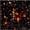 |
Fig. 1 VLT NACO JHKs composite image of the Quintuplet cluster. Outside the dotted rectangle only H- and Ks-band data are available. The dashed circle with a radius of 500 pixel or 0.5 pc indicates the region used for the derivation of the mass function (see Sect. 5.2). Due to bad AO correction, the J-band dataset was unsuitable to perform photometry and astrometry and was used only for this composite image. |
Standard data reduction was performed using a custom made reduction pipeline written in Python, calling a series of self-written IDL routines as well as PyRAF tasks12. Both sky and science frames were reduced by subtracting the appropriate darks and dividing by the twilight flat fields. A master sky image was created for each dataset by removing the brightest pixels from the stack of sky images to avoid contamination with stellar light. This is particularly crucial along the line of sight towards the GC, where the high stellar density prohibits the choice of star-free sky fields. Before the master sky image was subtracted from a science frame, it was scaled to the background level of this frame. Hot and dead pixels were detected from outliers during the combination of the dark images and twilight flats and written to the master bad pixel mask. For each science frame, pixels affected by cosmic ray hits were determined by the IRAF task cosmicrays and added to the master bad pixel mask to create an individual mask for each frame. The correction and treatment of specific detector related noise and ghost patterns is described in Appendix A.
The science frames of each dataset were combined with the IRAF task drizzle (Fruchter & Hook 2002). Each science frame was linearly weighted by the inverse of the full width at half maximum (FWHM) of an unsaturated, bright star present in all frames of this dataset in order to optimise the spatial resolution in the combined image. The large number of 44 exposures for the second epoch allowed for using only the 33 frames with a FWHM < 0.082″ in order to enhance the spatial resolution without losing stars at the faint end.
3. Photometry
3.1. Source extraction
Stellar fluxes and positions were determined with the starfinder algorithm (Diolaiti et al. 2000), which is designed for high precision astrometry and photometry on AO data of crowded fields. The point spread function (PSF) is derived empirically from the data by median superposition of selected stars after subtraction of the local background and normalization to unit flux. Using an empirical PSF is preferable for astrometric AO data, as the steep core and wide halo are not well reproduced by analytic functions. Stars whose peak flux exceed the linearity limit of the detector and are included in the list of stars for the PSF extraction are repaired by replacing the saturated core with a replica of the PSF, scaled to fit the non-saturated wings of the star3. Only if the saturated stars are repaired, they are definitely detected and fitted by the algorithm, so that their contribution on the flux of neighbouring stars can be subtracted. This is of special importance for faint stars located within the halo of a saturated star in order to measure their fluxes precisely. As spatially varying PSFs are not supported in starfinder, the PSF was assumed to be constant across the field (but see Sect. 3.2). Isolated, bright stars uniformly spread across the image were selected for PSF extraction. All saturated stars were included in the list of PSF stars in order to be repaired. The total number of selected PSF stars and the number of saturated stars among them are listed in Table 2. The comparably small number of saturated stars of the last dataset is due to the higher linearity limit of the Aladdin3 detector.
Number of stars for PSF extraction.
3.2. Relative photometric calibration
The simplification of a constant PSF across the whole image led to spatially varying PSF fitting residuals and in turn to small-scale zeropoint variations across the field. This is typical for AO data and is mostly a consequence of anisoplanatism at increasingly larger distances from the natural guide star. As the extracted PSF resembles an average of the different PSFs across the image, the variation of the residuals after PSF subtraction is not centred at the position of the guide star. In the case of both the 2003 and 2008 data, the residual image showed a radial variation of the PSF fitting residual overlaid with slow azimuthal changes. In order to correct for these local zeropoint variations, a spatially varying correction factor was determined from the flux ratio FR of the residual flux in the PSF subtracted image and the stellar flux within an aperture around the centroids of isolated stars. The flux ratio FR was fitted in dependence of the distance to the image centre for angular sectors of 45° (0°−45°, 45°−90°, ...) either by a constant offset or a small linear trend. The correction factor fcorr(r), which is to be multiplied to the fluxes of all stars within an angular sector, follows from the respective fit of the flux ratio FRfit(r): 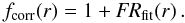 (1)The error of fcorr(r) is identical to the fitting error of FRfit(r), which is ΔFRfit(r) = Δc if the flux ratio in the respective angular sector was fitted by a constant offset c and
 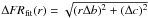 if the flux ratio was fitted by a linear trend with FRfit(r) = br + c.
This procedure resulted in the most consistent photometric calibration across the observed field. Besides the small-scale zeropoint variations the spatial variation of the PSF affects the centroiding accuracy of detected stars. This effect is described in Sect. 5.2.
3.3. Absolute photometric calibration
Reference sources for the photometric calibration were taken from the Galactic Plane Survey (GPS; Lucas et al. 2008), which is part of the UKIRT Infrared Deep Sky Survey (UKIDSS; Lawrence et al. 2007). Magnitudes of stars within the UKIDSS catalogue are determined from aperture photometry using an aperture radius of 1″ and are calibrated using the Two Micron All Sky Survey (2MASS; Skrutskie et al. 2006). Data from the Sixth Data Release (DR6) for the Quintuplet cluster was retrieved from the UKIDSS archive (Hambly et al. 2008). For a set of calibration stars (29 in H-, 13 in Ks-band), which could unambiguously be assigned to calibrated sources in the UKIDSS catalogue, the individual zeropoints were determined. Due to the high spatial resolution of the NACO data several fainter stars can be resolved within the UKIDSS 1″ aperture around each calibrator. As these stars do contribute to the measured flux in the UKIDSS aperture, the PSF-flux of all stars falling within a radius of r = 1″−0.5 × FWHMPSF, where FWHMPSF is the FWHM of the extracted NACO PSF, was added and compared to the magnitude of each calibrator in the UKIDSS catalogue. The final zeropoint was then determined from the average of the individual zeropoints of the calibration stars. The zeropoints of the two Ks-band datasets from the first epoch were determined subsequently using the calibrated second epoch data. No significant colour terms were found between the NACO H, Ks and the UKIDSS H, K filter systems.
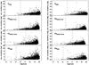 |
Fig. 2 Plot of the astrometric uncertainty (left panels) and the photometric uncertainty (right panels) vs. the magnitude for all four NACO datasets. The plotted photometric uncertainty does only include the PSF fitting uncertainty. The dashed lines mark the linearity limit of the respective dataset. |
3.4. Error estimation
The estimation of the photometric and astrometric uncertainties follows the approach described in Ghez et al. (2008) and Lu et al. (2009). The reduced science frames for each dataset were divided into three subsets of comparable quality and coverage. Each subset of 5 (first epoch) or 11 frames (second epoch) was combined with drizzle and the photometry and astrometry of the resulting auxiliary image was derived with starfinder in the same way as for the deep images. The photometric and astrometric uncertainty was derived as the standard error of the three independent measurements for each star detected in all three auxiliary frames. As no preferential direction is expected for the positional uncertainty, the astrometric uncertainty of each star is computed as the mean of the positional uncertainty in the x- and y-direction. The astrometric and photometric uncertainties as derived from the auxiliary frames are shown in dependence of the magnitude in Fig. 2 for all datasets.
In order to remove false detections from the three Ks-band catalogues, only stars which were detected in all three auxiliary images of the respective dataset, and hence with measured astrometric and photometric uncertainties assigned, were kept in the respective source catalogue. For the H-band data this criterion was not applied. The H-band was matched (see Sect. 6) with a Ks-band catalogue containing only stars detected in both epochs. It is assumed that a star found in the Ks-band images of both epochs is a real source and if it is missing in one of the H-band auxiliary images this is a consequence of the substantially lower photometric depth of the auxiliary image.
The photometric errors as stated in the final source catalogue (Table 4) do include the respective zeropoint uncertainties, the photometric uncertainties due to the flux measurement from PSF fitting, and the error of the correction factors (Sect. 3.2).
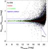 |
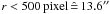
Fig. 3 Difference of the inserted and recovered magnitudes of artificial stars inserted into the combined image of the Ks-band data in 2008 plotted vs. the magnitude. A high-order polynomial fit to the median and the standard deviation (multiplied by a factor of 1.5) of the magnitude difference within magnitude bins of 1 mag are shown as well. The vertical dotted line indicates the maximum Ks-band magnitude at Ks = 19 mag of stars to be used for the proper motion analysis. |
4. Completeness
In order to quantify the detection losses due to crowding effects, the local completeness for each dataset was determined from the recovery fraction of artificial stars inserted into each combined image. The artificial star experiment for the H-band data covers a magnitude range from 9.5 to 21.5 mag. For each magnitude bin with a width of 0.5 mag, 42 artificial star fields were generated. Each artificial star field was created by adding 100 artificial stars, which are scaled replica of the empirical PSF, inserted at random positions and with random fluxes within the respective flux interval, into the combined image.
For the three Ks-band datasets, the artificial stars were inserted at the same physical positions as in the H-band image and with a magnitude in Ks yielding a colour for the respective artificial star of H − Ks = 1.6 mag, which resembles the colour of main sequence (MS) stars in the Quintuplet cluster (see Sect. 6). The photometry on the images with added artificial stars was performed in the same way as for the original images. In addition to artificial stars which were not re-detected by starfinder, stars, whose recovered magnitudes deviated strongly from the inserted magnitudes, were considered as not recovered. The criterion to reject recovered stars due to their magnitude difference between input and output magnitude was derived from polynomial fits to the median and the standard deviation of the magnitude difference within magnitude bins of 1 mag (Fig. 3). Stars with absolute magnitude differences larger than 1.5 times the fit to the standard deviation are treated as not recovered, but only if their absolute magnitude difference exceeds 0.20 mag. The median of the magnitude difference exposes a systematic increase towards the faint end, exceeding 0.05 mag for Ks > 19.4 mag or H > 20.25 mag. This trend indicates that for the faintest stars the measured fluxes contain systematic uncertainties. As we restrict the analysis to stars brighter than Ks < 19 mag, sources at these faint magnitudes are excluded from the proper motion and mass function derivation.
The left panel in Fig. 4 shows the overall recovery fraction for all datasets (Ks 2003 and 2008, and H 2003) within a radius of 500 pixels ( ) from the image centre, the part of the image actually used for the determination of the present-day mass function (see Sect. 5.2). The recovery fraction for the Ks-band data from 2003 is a combination of the recovery fractions for the two Ks-band datasets of that epoch. The dataset with the longer DIT of 20.0 s is used only for magnitudes fainter than the linearity limit of this dataset at 14.3 mag. For brighter magnitudes, the recovery fraction of the 2003 Ks-band data with the short DIT of 2.0 s is drawn. The total recovery fraction also shown in the figure is the product of all three recovery fractions and is most relevant for the completeness correction of the mass function, as i) only stars which are detected in both epochs can be proper motion members and ii) only for stars with measured H-band magnitudes can masses be derived reliably.
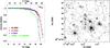 |
Fig. 4 Left panel: recovery fractions of artificial stars inserted within the inner 500 pixel from the centre of the observed field plotted vs. the respective magnitude in the Ks- (lower abscissa) or H-band (upper abscissa). The full and dotted lines correspond to the recovery fractions for the Ks-band data in 2003 and 2008, respectively and the dash-dotted line shows the completeness in the H-band. The dashed line shows the total completeness for the stars after matching the two Ks-band and the H-band datasets. Only stars with Ks < 19 mag are used for the proper motion analysis, as indicated by the vertical dotted line. Right panel: Ks-band image from the second epoch with the overplotted contours representing a completeness level of 50% for the labelled magnitudes. |
Completeness varies as a function of position due to the non-uniform distribution of brighter stars and hence is a function of the stellar density and magnitude contrast between neighbours (see e.g., Eisenhauer et al. 1998; Gennaro et al. 2011). A spatially-dependent approach to determine the local completeness value becomes especially important if the cluster exhibits a non-symmetric geometry or in the presence of very bright objects, which heavily affect the completeness values in their surrounding. Both effects are present in the Quintuplet cluster. In order to assign a local completeness value to each detected star, the method described in Appendix A of Gennaro et al. (2011) was applied to derive completeness maps for each combined image containing the recovery fraction for every pixel as a function of magnitude. The procedure encompasses three steps performed for each magnitude bin (for a detailed description the reader is referred to Gennaro et al. 2011): 1.) determine for each artificial star its ν nearest neighbours among the inserted stars (ν = 16 for all datasets). The local, averaged completeness value at the position of the considered artificial star follows from the fraction of the recovered nearest neighbours (including the star itself); 3.) interpolate these local completeness values into the regular grid of image pixels; 4.) smooth the obtained map with a boxcar kernel with a width of the sampling size in order to remove potential artificial features introduced by the previous step. The sampling size ⟨ d ⟩ is the typical separation of independent measurements of the local completeness value and depends on the image area A, the number of inserted stars N and the chosen number of nearest neighbours ν (see Eq. (A1) in Gennaro et al. 2011): 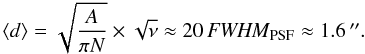 (2)For the final step the completeness maps of all magnitude bins are used. To ensure that the completeness decreases monotonically with increasing magnitude, a Fermi-like function is fitted to the completeness values at every pixel in the image as a function of magnitude. The completeness (or recovery fraction) for every real star can then be computed from the fit parameters at the position of the star in each image. The right panel in Fig. 4 shows the combined Ks-band image for the 2008 epoch with superimposed 50%-completeness contours and limiting magnitudes labelled. The very bright stars with their extended halos hamper the detection of nearby faint stars causing the recovery fraction to be non-uniform across the field, as expected. The completeness of a star entering the mass function is the product of its completeness in the H-band, the 2008 epoch Ks data, and either the 2.0 s DIT (Ks,2003 < 14.3 mag) or the 20.0 s DIT (Ks,2003 > 14.3 mag) 2003 epoch Ks dataset as determined from the respective completeness maps:
  (3)For stars brighter than H = 13.5 mag or Ks = 10.4 mag the completeness was assumed to be 100%.
5. Proper motion membership
Due to the high field star density for lines of sight towards the GC the distinction between cluster and field stars becomes particularly important. As most of the field stars are located within the Galactic bulge they have similar extinction values as the cluster and cannot be distinguished from cluster members on the basis of their colours alone. The high astrometric accuracy of the AO assisted VLT observations in combination with the time baseline of 5.0 yr allows for the measurement of the individual proper motions of stars at the distance of the Quintuplet cluster. The primary applied method to discern the cluster members from the field stars is based on the measured proper motions.
5.1. Geometric transformation
In order to determine the spatial displacements, two geometric transformations were derived to map each position in the two first epoch Ks images (2003) with short (2.0 s) and long (20.0 s) DIT onto the corresponding position in the second epoch Ks image (2008). The second epoch is used as reference epoch because of the higher astrometric accuracy, deeper photometry and brighter linearity limit of this dataset. Only the Ks-band datasets were used to determine the spatial displacements, as due to their higher Strehl ratios the stellar cores are better resolved than in H-band, providing the better centroiding accuracy and hence most accurate astrometry.
Under the assumption that internal motions are not resolved so far, the cluster itself served as the reference frame. The geometric transformation was derived in an iterative process. First, a rough transformation was determined with the IRAF task geomap using the positions of manually selected bright, non-saturated stars uniformly distributed across the images of both epochs. The respective catalogue of the first epoch dataset (2003) was then mapped onto the catalogue of the second epoch (2008) to get a mutual assignment of stars found in both catalogues. From these stars the most likely cluster candidates were selected to provide the reference positions for the refined, final geometric transformation. As the bright stars used for the preliminary transformation are likely cluster members, the distribution of spatial displacements in the x-, y-direction of cluster star candidates are expected to scatter around the origin. Therefore, only stars with spatial displacements within a radius of  from the origin were selected for the derivation of the final transformation, which excludes most of the presumed field stars. Further, as the bulk of cluster stars are probably brighter than most stars in the field, only non-saturated bright and intermediate bright stars (11.5 < Ks < 15.5 mag for a DIT of 2.0 s and 14.0 < Ks < 17.0 mag for a DIT of 20.0 s) provide the reference positions. The final geometric transformations were derived with geomap in an interactive way. The residual displacements in the x-, y-directions between the transformed first epoch and the second epoch coordinates were minimized by iteratively removing outliers and carefully adapting the order of the polynomial fit (=3 for the final transformations). The final rms deviation of the geometric transformation was 0.2 mas/yr in the x- and 0.3 mas/yr in the y-direction for the dataset with a DIT of 2.0 s, and 0.3 mas/yr in the x- and y-direction for the dataset with a DIT of 20.0 s. For a total cluster mass of Mcl ≈ 6000 M⊙ within a radius of r ≤ 0.5 pc (see Sect. 8) the internal velocity dispersion is expected to be of the order of 0.15 − 0.2 mas/yr or 6 − 8 km s-1. As this is smaller than the uncertainty of the geometric transformation alone, intrinsic motions are not resolved. Therefore the selection of cluster stars as geometric reference sources is justified.
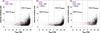 |
Fig. 5 Left panel: plot of the combined astrometric uncertainty from the two epochs of Ks-band data plotted vs. the magnitude of the second epoch (for details of the error estimation see Sect. 3.4). The median and standard deviation of the astrometric uncertainty above the linearity limit (at 14.3 mag) of the dataset in 2003 with 20.0 s DIT were fitted by polynomials. This fit of the median (lower line) and the sum the median and standard deviation (upper line) are drawn in all three plots. Middle panel: astrometric uncertainty of stars residing within a circle with |
5.2. Data selection and combination
Each of the two transformed star catalogues of the Ks-band data from the first epoch was matched with the star catalogue of the second epoch using a matching radius of 4 pixels ( ). The matching radius was chosen small enough to avoid mismatches between close neighbouring stars, but large enough to include all moving sources at GC distances below the escape velocity of the GC. A displacement of 108 mas within the time baseline of 5.0 yr for a distance of 8.0 kpc to the GC (Ghez et al. 2008) corresponds to a proper motion of 820 km s-1. The combined astrometric uncertainty
 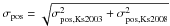 was derived for both of these catalogues. In the left panel of Fig. 5, the combined astrometric uncertainty is plotted against the magnitude. The datapoints below the linearity limit of the long exposure in 2003 at Ks = 14.3 mag originate from the match of the second epoch with the data with a DIT of 20.0 s, the datapoints at brighter Ks magnitudes are from the match with the data obtained with a shorter DIT of 2.0 s. For the matched catalogue using the first epoch dataset with a DIT of 20.0 s, the median and the standard deviation of the astrometric uncertainties within bins of 0.5 mag width were fitted by a third and second order polynomial, respectively. The fit to the median and the sum of both fits are shown in all three panels of Fig. 5 for comparison. The usage of one averaged PSF for the whole image results in the observed radial increase of the PSF fitting residuals (see Sect. 3.2). The centroiding accuracy is therefore expected to decrease towards larger radii resulting in a larger astrometric uncertainty. The centre and right panel of Fig. 5 exemplify this behaviour by using only stars with a distance of less than or greater than
  from the centre of the combined images in both epochs, respectively. The decrease in the scatter and magnitude of the astrometric uncertainties at smaller radii is striking. The median of the astrometric uncertainty for 12 < Ks < 18 mag is 1.46 mas for stars within a radius of 500 pixel, but 2.64 mas for stars outside that radius. Therefore, the further analysis is restricted to stars within a radius of 13.6″ from the centre of the observed field of view for the remainder of this paper. The astrometric uncertainties rise steeply near the detection limit at about 20 mag (see centre panel in Fig. 5). For stars fainter than 19 mag, almost no stars exhibit an uncertainty below the median value of stars with intermediate brightness (14 < Ks < 17 mag). Stars with a Ks-band magnitude fainter than 19 mag are therefore excluded from the sample. As last selection based on the combined uncertainty, stars fainter than Ks = 14.3 mag are removed if their uncertainty is above the sum of the fits of the median and standard deviation derived from the combined uncertainty of all observed stars (see Fig. 5). The percentage of rejected stars varies between 0 and 9.4% for the affected magnitude bins and does not show a systematic trend with magnitude, therefore no systematic bias is introduced by this selection. After the above mentioned selections, the two matched catalogues were combined. Stars fainter than Ks = 14.3 mag were taken from the match with the DIT 20.0 s first epoch data, brighter stars originate from the matched catalogue using the dataset from the first epoch with a DIT of 2.0 s. The final Ks-band catalogue contains a total of 1304 stars.
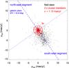 |
Fig. 6 Proper motion diagram of stars with Ks ≤ 19 mag. The dashed line marks the direction parallel to the Galactic plane, the dotted line is oriented vertically with respect to the Galactic plane and splits the proper motion diagram into the north-east and the south-west segment. Stars within a radius of 2σ as derived from the Gaussian fit in Fig. 7 (right panel) around the origin are selected as cluster members. |
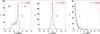 |
Fig. 7 Left panel: histogram of proper motions parallel to the Galactic plane. Middle panel: histogram of proper motions vertical to the Galactic plane. Right panel: histogram of the 2-dimensional proper motions located in the north-east-segment of the proper motion diagram. The histogram was fitted with a Gaussian function and a 2σ cut was used as the selection criterion for cluster membership (dash-dotted lines in all three panels). |
5.3. The proper motion diagram
Individual stars are plotted in the proper motion diagram (Fig. 6) with proper motions in the east-west-direction on the x- and proper motions in the north-south direction on the y-axis. As the cluster is used as the reference frame, the distribution of cluster members is centred around the origin and overlaps with the elongated distribution of the field stars. The orientation of the field stars is approximately parallel to the plane of the Galaxy (dashed line in Fig. 6). The dotted line running through the origin and vertically to the Galactic plane splits the proper motion diagram into two halfs being referred to as the north-east segment (upper half) and the south-west segment (lower half).
Figure 7 shows histogram plots of the distribution of the proper motions parallel (left panel) and vertical to the Galactic plane (centre panel). The distribution of proper motions in the direction parallel to the Galactic plane is strongly peaked at the origin, with a very steep decline in the north-west segment, and a slightly broadened decline and overlap with the broad field star distribution in the south-west segment, as expected from Fig. 6. The proper motions vertical to the Galactic plane are almost distributed symmetrically with respect to the Galactic plane (centre panel in Fig. 7), confirming the assumed orientation of the field star distribution in the proper motion diagram. This and the exposed offset of the field star distribution in the proper motion diagram indicate a movement of the Quintuplet Cluster parallel to the Galactic plane towards the north-east with respect to the field as was found previously for the Arches Cluster (Stolte et al. 2008). The sample of stars with proper motions in the north-east segment is least contaminated by field stars and was therefore used to derive the membership criterion. The distribution of proper motions in the north-east segment was fitted with a Gaussian function (right panel in Fig. 7). Stars whose proper motions are within a circle of radius 2σ = 2.26 mas/yr, where σ is the width of the Gaussian fit, are selected as cluster members (see Fig. 6). Two of the initial five Quintuplet members (Q1, Q9; Nagata et al. 1990; Okuda et al. 1990) do not fall inside this circle. Their fluxes are exceeding the linearity limits by a factor of 8–30, such that their positions are not well determined. Note that this only affects the very brightest sources, for which spectroscopic member identification is available (Figer et al. 1999b; Liermann et al. 2009). These two stars were added manually to the sample of proper motion members.
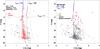 |
Fig. 8 Left panel: colour–magnitude diagram of cluster member candidates on the basis of their proper motions. A 4 Myr isochrone with solar metallicity, combined using a Padova MS-isochrone and a Pisa-FRANEC PMS-isochrone, shifted to a distance of 8 kpc and a foreground extinction of AKs = 2.35 mag, is shown for reference. Stars, with fluxes exceeding the linearity limit of the detector are drawn as crosses in all figures throughout this paper. A two-step colour-cut was applied for stars with H > 14 mag to remove field stars with similar proper motions as the cluster from the cluster sample (see Sect. 6 for details). The vertical short-dashed lines mark the first colour-cut, while in the second step of the colour-cut highly reddened objects to the right of the second isochrone (AKs = 2.89 mag, long-dashed line) are removed. The dots represent the sample of cluster stars after the colour-cut, stars rejected based on their colour are drawn as triangles. Spectroscopically identified field supergiants from the LHO catalogue (Liermann et al. 2009) are marked with diamonds and are removed from the final cluster sample. Right panel: colour–magnitude diagram of stars classified as belonging to the field according to their proper motion (dots) and of stars removed from the member sample based on their colour or known spectral type (triangles). One star, classified as belonging to the field by its proper motion, has an O-star as (ambiguous) counterpart in the LHO catalogue (see Sect. 6) and is marked with a circle. The tilted dotted line is the line of reddening according to the extinction law by Nishiyama et al. (2009) running through the population of red clump stars from the Galactic bulge. |
6. Colour–magnitude diagrams
The Ks source catalogues of proper motion members and non-members were matched with the source catalogue of the first epoch H-band data. The corresponding CMDs are shown in Fig. 8 and use only magnitudes in H and Ks from the first epoch to avoid additional scatter being introduced by variable stars. Stars whose fluxes exceed the respective linearity limit in either H and/or Ks at H = 12.05 mag and Ks = 11.25 mag are marked with crosses. All 1221 stars (member and non-members) with measured proper motion and (H − Ks) colour are included in the final source catalogue (see Table 4).
Cluster and field stars separate well as can be seen by characteristic features of the field population (right panel), that are absent in the cluster selection (left panel). For example an elongated overdensity is observed, which starts at about H = 17 mag, H − Ks = 1.8 mag and extends to redder colours along the reddening path adopting the extinction law by Nishiyama et al. (2009). It is consistent with arising from red clump stars located in the Galactic bulge. Assuming the intrinsic K-band magnitude for red clump stars of K = −1.61 mag by Alves (2000), the assumed intrinsic colour of H − Ks = 0.07 of Nishiyama et al. (2006), a distance to the GC of 8 kpc (Ghez et al. 2008) and an approximate extinction of AKs = 2.35 mag, which is also appropriate for the cluster MS (see Sect. 7), yields HRC = 17.05 mag and (H − Ks)RC = 1.79 mag.
Several blue foreground stars with colours H − Ks ≤ 1.3 mag are seen to the left of the cluster member sequence (Fig. 8, left panel). These sources are likely disc main sequence stars following the differential rotation of the outer Milky Way rotation curve. With expected velocities of ~200 km s-1, they cannot be distinguished from the cluster population on the basis of their proper motion alone. Furthermore a few very red objects, which could be non-members by comparison with the field CMD, remain in the proper motion sample. In order to remove these contaminants a two-step colour-cut was applied to stars fainter than H = 14 mag. First the blue foreground and red background stars were removed by keeping only stars with 1.3 ≤ H − Ks ≤ 2.3 mag. In a second step the individual extinction of the remaining stars fainter than H = 14 mag was determined from the intersections of the lines of reddening with a 4Myr isochrone assuming a distance to the cluster of 8 kpc. The method to derive the individual extinction and the used isochrone are explained in detail in Sect. 7. The isochrone was shifted to an extinction of AKs = 2.89 mag, corresponding to the sum of the mean ( ) and twice the standard deviation (σAKs = 0.24 mag) of the individual extinctions of the cluster members remaining after the first colour-cut, and stars redder than the shifted isochrone were also removed from the sample of cluster stars.
The designated cluster members and non-members were compared with the K-band spectral catalogue of Liermann et al. (2009, hereafter LHO catalogue) for a spectral classification of the brighter stars and in order to assess the selection of cluster stars based on their proper motions and colours. Only observed stars with a Ks-band magnitude brighter than 15.5 mag, which is about 1 mag fainter than the faintest star in the LHO catalogue, were included in the comparison. Eighty-five stars from the spectral catalogue could be assigned to 92 observed stars (69 members, 23 field stars). The ambiguous assignments of 6 stars from the LHO catalogue to 13 observed stars (all members) are caused by the lower spatial resolution of the SINFONI-SPIFFI instrument of 0.250″ for the used 8″ × 8″ field of view. The spectral classification for the matched stars is indicated in a simplified form by the overplotted symbols in Figs. 8–10. Stars with ambiguous assignments are additionally marked with an X-cross. One star (LHO 110) was re-classified in Liermann et al. (2010) from O6-8 I f to WN9h and is treated accordingly in the figures. The numbers and spectral classifications from the LHO catalogue are noted in the source catalogue (Table 4). Six late-type M, K supergiants are still contained within the cluster sample after the colour-cut and are very likely remaining contaminants with motions similar to the cluster members from the Galactic bulge considering the young age of the cluster. These stars and stars rejected by the colour-cut were removed from the final cluster sample and added to the proper motion non-members in the field star CMD (plotted as triangles in the right panel of Fig. 8). The one early-type star (O4-7 I f) among the designated field stars is located at the edge of the analysed area of the data and very close to a second star just outside this region. It is therefore unclear if the spectral classification really belongs to this star or its neighbour, hence the star was not added to the final cluster sample. For 12 of the 62 stars in the LHO catalogue, which could be assigned to designated cluster members, the sources in our catalogue exceed the Ks-band linearity limit by more than 1 mag. This impedes the repair of the core by starfinder and the correct measurement of the position and proper motion. Disregarding these 12 stars, the percentage of contaminating M, K supergiants, which cannot be discerned from the cluster members based on their proper motion or colour, amounts to 6/(62 − 12) = 12%. Even after the removal of the 6 M, K supergiants some field stars may still remain in the final cluster sample, as only down to about H = 15.5 mag most stars have a counterpart in the LHO catalogue. The number of these contaminants is estimated in Appendix C.
The CMD of the final sample of cluster stars is shown in Fig. 9 and, separated into the north-east and south-west segment of the proper motion diagram, in Fig. 10. The slight overdensity located at H − Ks = 1.8 mag, H = 17 mag indicates a remaining contamination with red clump stars, which is more pronounced for stars with proper motion in the south-west segment. The CMD for the south-west segment contains 94 stars more than for the north-east segment mainly at the faint end of the observed population, which appears slightly broadened. This is expected from the proper motion diagram as the field star population overlaps with the cluster stars in the south-west segment causing a larger contamination for this segment. The astrometric uncertainty and therefore the scatter in the proper motion diagram increases for fainter magnitudes and therefore the confusion with faint field stars is more severe. The cluster members in the north-east segment therefore constitute the cleanest sample.
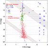 |
Fig. 9 Colour–magnitude diagram of the final cluster sample. Stars with counterparts in the LHO catalogue are flagged with symbols according to their spectral type (box: WR-stars, circle: OB-stars, stars with ambiguous identification are additionally marked with an X-cross). The horizontal dashed and short-dashed lines mark the initial masses along the isochrone in units of M⊙. The tilted dotted lines show the lines of reddening according to the extinction law by Nishiyama et al. (2009) and enframe the two regions in the CMD (shaded in grey in Figs. 9–11), within which the isochrone has multiple intersections with the line of reddening, and consequently no unique mass can be inferred for a given star. |
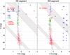 |
Fig. 10 Colour–magnitude diagram of all stars of the final cluster sample with proper motions residing in the north-east (left panel) or south-west segment (right panel) of the proper motion diagram (Fig. 6). See Figs. 8 and 9 for details. |
 |
Fig. 11 Comparison of the four isochrones used to determine stellar masses. For all shown isochrones, solar metallicity, a distance to the cluster of 8 kpc and a foreground extinction of AKs = 2.35 mag is adopted. As in Figs. 9 and 10, the dotted lines enframe regions in the CMD with ambiguous mass assignments (shaded in grey) and the initial masses are labelled along the isochrones. |
7. Mass derivation
Based on the presence of WC stars, O I stars and a red supergiant within the Quintuplet cluster, Figer et al. (1999b) derived an average age of 4 ± 1 Myr assuming a coeval population. More recently the ages of 5 WN stars were determined by comparison of their luminosities and effective temperatures as derived from spectral line fitting with stellar evolution models to be about 2.4 − 3.6Myr pointing to a somewhat younger age of the cluster (Liermann et al. 2010). To study the influence of the assumed cluster age on the slope of the mass function, three isochrones with ages of 3, 4 and 5 Myr were used to derive the initial stellar masses. The isochrones are a combination of Padova main sequence (MS) isochrones and pre-main sequence (PMS) isochrones derived from Pisa-FRANEC PMS stellar models (see Gennaro et al. 2011; Marigo et al. 2008; Degl’Innocenti et al. 2008). As the NACO photometry is calibrated by means of UKIDSS sources (see Sect. 3.3), the combined isochrones, for simplicity referred to as 3, 4 and 5 Myr Padova isochrones in the following, were transformed from the 2MASS into the UKIDSS photometric system using the colour equations from Hodgkin et al. (2009, Eqs. (6)–(8)). To cover the effect of a different set of stellar models on the derived masses, a 4 Myr Geneva MS isochrone with enhanced mass loss for high mass stars, M > 15 M⊙, Lejeune & Schaerer (2001) was included in the comparison. The conversion of this isochrone into the UKIDSS filter system encompassed two steps. The isochrone was first transformed from the Bessell & Brett (1988) to the 2MASS photometric system using the updated4 transformation by Carpenter (2001) and subsequently from the 2MASS to the UKIDSS filter system using the above mentioned conversion.
For all isochrones, solar metallicity according to the description of the underlying stellar models5 was assumed, and a distance to the GC of 8.0 kpc (Ghez et al. 2008) was applied as the distance to the Quintuplet cluster. The four isochrones shown in Fig. 11 were reddened by a foreground extinction of AKs = 2.35 mag using the extinction law of Nishiyama et al. (2009) (AH:AKs = 1.73:1) to match the observed MS of the cluster members. This extinction law is one of the most recent determinations of the extinction in the near-infrared along the line of sight towards the GC and consistent with other current findings, e.g., by Straižys & Laugalys (2008) or Schödel et al. (2010).
The individual mass and extinction of each star in the final cluster sample was determined from the intersection of the line of reddening through the star with the respective isochrone in the CMD. Due to the local maximum of the PMS at the low-mass end as well as the extended loop at the transition from the end of the hydrogen core burning to the contraction phase at the high-mass end, the de-reddening path of a star may have several intersections with the isochrone, thus leading to an ambiguous mass assignment (the affected areas in the colour-magnitude plane are shaded in grey in Figs. 9–11). For these stars, the masses at each intersection were averaged. The post-MS phase after the exhaustion of hydrogen in the stellar core is very rapid (a few 103 yr according to the stellar models) and apparent in the isochrones as the branch with increasing H-band brightnesses, re-rising after the decline connected to the contraction phase. Due to its short duration, which causes the Hertzsprung gap in the Hertzsprung-Russel diagrams of stellar clusters, only the two intersection points with the upper part of the MS and with the subsequent falling branch of the isochrone were averaged. Two O stars from the LHO catalogue have no intersection with the Geneva isochrone on the MS or the falling branch, therefore an initial mass of 47.3 M⊙, which is the maximum mass along this isochrone used for the mass determination (see Table 3), was assigned to them.
Eleven Wolf-Rayet stars out of the 21 observed in the Quintuplet Cluster are contained within our sample of cluster members. The masses for these stars could not be determined from the isochrones but the mass range of Wolf-Rayet stars was inferred from the underlying stellar models by Bressan et al. (1993) for the Padova isochrones and by Meynet et al. (1994) and Schaller et al. (1992) for the Geneva isochrone (see Table 3).
Considering only stars above the PMS/MS transition region, the individual extinction AKs of each star as inferred from the 3, 4 and 5 Myr Padova isochrones agrees within ± 0.02 mag ( ± 0.005 mag for 5.5 < m < 30 M⊙). Using the 4 Myr Geneva isochrone yields systematically smaller values of the individual extinction by 0.08 − 0.12 mag. The individual extinction value denoted in the final source catalogue (Table 4) refers to the 4 Myr Padova isochrone.
Summary of isochrone properties relevant for the mass derivation.
Catalogue of stellar sources with measured proper motions and colours in the Quintuplet cluster.
8. Mass functions
In order to avoid potential biases introduced by bins with a very small number of objects or large differences in the number of stars between the low- and high-mass bins, we adopted the method proposed by Maíz Apellániz & Úbeda (2005). Here, the widths of the different bins are adjusted such that each bin houses approximately the same number of stars (Method A). If the number of stars in the sample did not split up evenly for the chosen number of bins, the bins to contain one additional star from the remaining stars were chosen randomly. The stars were then sorted according to their masses and distributed among the bins. For each isochrone the mass function (MF) and slope were determined for dividing the cluster sample into 4, 8, 12, 16 and 20 bins. The boundary between two adjacent bins was set to the mean of the most/least massive star in the respective bins. The minimum mass used for each mass function was set to the lowest mass of a star with a unique mass assignment for the respective isochrone, i.e. lying above the ambiguity region caused by the PMS/MS transition. Stars with ambiguous mass assignments at the upper end of the MS were kept for the mass function, as due to their small number they all contribute to the uppermost bin in the mass function. The upper mass limit or uppermost bin boundary mup was calculated from the data to be (see Maíz Apellániz & Úbeda 2005)  (4)with n being the total number of stars. The number of stars in each bin ni was normalized by the respective bin width Δmi. The logarithm of the normalized number of stars per bin as a function of the logarithm of the medium mass of each bin was fitted with a straight line using the IDL routine LINFIT, which performs a χ2 minimisation.
The uncertainty of the number of stars per bin Δni is derived by Maíz Apellániz & Úbeda (2005) from the standard error of a binomial distribution (npi(1 − pi))1/2, where the unknown true probability for a star to reside in the ith bin pi is approximated by the measured value ni/n:  (5)Note that this uncertainty differs from the Poisson error
  , which is usually applied to binned data. For the linear fit each bin was weighted by its statistical weight wi = 1/Δni2. The statistical weight wi assigned to the logarithm of the normalized number of stars per bin (log 10(ni/Δmi)) follows from error propagation of Δni in the logarithmic plane (see Eq. (7) in Maíz Apellániz & Úbeda 2005):
  (6)It is basically the same for every bin as the number of stars per bin varies by a maximum of one.
Besides the binning method just described, the mass function was also determined using an equal logarithmic width for each bin (Method B), which is still the most common binning method for deriving mass function slopes (see Maíz Apellániz & Úbeda 2005, for a discussion of the biases of this method). The lower and upper mass limits were determined in exactly the same way as above and the logarithmic bin widths were set by dividing the so defined mass range into 4, 8, 12, 16 and 20 bins. The weights applied to each bin were again calculated with Eq. (6) and are decreasing going to higher masses due to the lower number of stars contained in the high mass bins. In order to study the influence of the weights on the slope for this binning method, the slope was derived from a linear fit to the MF with and without weighting.
The reported slopes of the mass function α refer to a power-law distribution in linear units (dn/dm ∝ mα) with the standard Salpeter slope being α = −2.35 in this notation (Salpeter 1955). If not mentioned otherwise, the mass function and its slope were determined using all cluster members from both the north-east and south-west segment (see Fig. 10) and distributing the stars into bins with (almost) constant number of stars (Method A). All shown linear fits to the respective mass functions were derived from the completeness corrected mass function using for each star its individual completeness correction (see Sect. 4).
The minimum mass of a star with unique mass assignment was 5.5, 4.6 and 4.0 M⊙ for the 3, 4 and 5 Myr Padova isochrone, respectively. The minimum mass for the 4 Myr Geneva isochrone was set to 4.5 M⊙ in order to use exactly the same stars as for the Padova isochrone of the same age. As mentioned in Sect. 7, it was not possible to infer the individual masses of the WR stars from the isochrones. Therefore, a constant mass within the mass ranges of the Wolf-Rayet stars deduced from the stellar models (see Table 3) was assigned to each identified Wolf-Rayet star in the cluster sample in dependence of the assumed cluster age. The uppermost bin boundary, calculated with Eq. (4), is then identical to the assigned WR mass. The chosen WR mass has a significant impact on the derived slopes due to the fairly large mass range of the Wolf-Rayet stars for cluster ages of 3 and 4 Myr. A larger assigned WR mass biases the mass function to a steeper slope due to the normalization of ni by the bin width Δmi. The maximum difference between the slopes using the minimum and maximum WR masses for each of the isochrones was 0.21, which is about twice the typical formal fitting error of the slope. To avoid the described bias, the Wolf-Rayet stars were not included in the mass function. After the exclusion of the Wolf-Rayet stars, the uppermost bin boundary is determined by the two most massive stars in the respective sample (see Eq. (4)).
In order to quantify the effect of the random selection of bins to contain one additional star from the remainder of the division of the total number of stars by the number of bins (Method A), the distribution process and the fit to the resulting MF was repeated 1000 times. The reported slopes for this binning method are the mean slope of all these repetitions. The maximum difference between the slopes of the same MF due to different random distributions of the surplus stars was 0.03, which is very small compared to the formal fitting errors.
The slope of the mass function of each isochrone was determined using 4, 8, 12, 16 and 20 bins. Using only 4 bins results in slopes being systematically shallower than for the other numbers of bins by up to 0.10. The choice of 20 bins introduces a bias in the case of the 3 Myr isochrone. Due to the large number of massive stars with averaged masses for this isochrone (see Table 3), these stars fill up the uppermost bin completely. The mass range of stars with averaged masses is compressed, which in turn leads to a decreased binwidth of the last bin. As the number of stars is normalized by the bin width, the normalized number of stars in the last bin is increased leading to a flatter slope. The most reliable mass function slopes are therefore obtained using 8, 12 or 16 bins. The maximum difference of the obtained slopes for a given isochrone between these three bin numbers was 0.03. Given this negligible influence of the bin number, all results presented in the following are determined using 12 bins (see also Table 5).
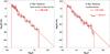 |
Fig. 12 Comparison of the mass function and derived slopes for different methods of binning the data and performing the linear fit. Only the fit and derived slope for the completeness corrected mass function are shown. Left panel: mass function of the Quintuplet cluster with initial masses derived from the 4 Myr Padova isochrone. Only stars with m > 4.6 M⊙, i.e. stars above the ambiguity region in the CMD due to the PMS, are used. Wolf-Rayet stars are not included in the mass function, as the large uncertainty of their mass might bias the derived slopes. The bin sizes are adjusted such that each of the 12 bins holds approximately the same number of stars. Right panel: mass function of the same data but distributing the stars into 12 bins of a uniform logarithmic width of 0.084 dex adopting the same lower and upper mass limits as in the left panel. The solid line shows the weighted linear fit, the dotted line the unweighted fit. |
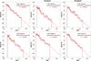 |
Fig. 13 Upper panels: mass functions for the 4 Myr MS-Padova isochrone using all stars (left), or only stars located in the north-east- (middle), or south-west-segment (right) of the proper motion diagram (Fig. 6). Lower panels: resulting mass function if stellar masses are derived from a 3 or 5 Myr Padova MS-isochrone (left and middle) or 4 Myr Geneva isochrone (right). For all shown mass functions the stars were distributed in 12 bins of variable width with equal numbers of stars per bin. As in Fig. 12, the Wolf-Rayet stars were removed and only stars above the ambiguity region in the CMD due to the PMS are included. The resulting minimum masses are 5.5, 4.6, 4.0, and 4.5 M⊙, for the 3, 4, 5 Myr Padova and the 4 Myr Geneva isochrone, respectively. |
Overview of derived slopes of the mass function binning the data into 12 bins containing approximately the same number of stars.
Figure 12 shows the comparison of the mass functions and the derived slopes for distributing the data in bins with (almost) constant number of stars (Method A, left panel) and for using bins of equal logarithmic width of Δlog 10m = 0.084 dex (Method B, right panel) for the 4 Myr Padova isochrone. In the shown example and in general the three slopes of the weighted fit to the mass function derived with a uniform number of stars per bin and the weighted and unweighted fit to the mass function with an equal logarithmic bin width agree well within the errors, if the full sample of stars is fitted. The use of a constant logarithmic bin size with applied weights following the prescription of Maíz Apellániz & Úbeda (2005) generates consistent results compared to the use of bins with variable widths and equal numbers of stars also if only stars from the north-east or south-west segment of the proper motion diagram are included in the mass function. In contrast, the unweighted fit responds much more sensitively to fluctuations of the number of stars in the higher mass bins, especially if the last bin included in the fit is depleted, which is the case for the south-west segment. For the remainder of this paper only the results determined from mass functions with an equal number of stars per bin are considered.
The first row in Fig. 13 shows the mass function for the 4 Myr Padova isochrone for all cluster members (left panel), for stars in the north-east-segment (centre panel), and for stars in the south-west segment (right panel). All three slopes agree well, although a lack of stars in the mass function of the north-east segment in the mass range of 11−22 M⊙ compared to the south-west segment is evident. This surplus of stars for the south-west segment is also apparent in the CMD (Fig. 10) and could indicate a remaining contamination with red clump stars. Further contaminations suggested by the difference in the number of cluster members in the north-east and south-west segment are likely removed by only using stars with intermediate brightness and masses above 4.6 M⊙.
For the Padova isochrones the slope of the mass function decreases with increasing age going from 3 to 5 Myr from  to (−1.55 ± 0.09). As can be seen in Fig. 11, the range of initial masses along the upper part of the MS starting at about 20 M⊙ strongly decreases with age. This causes the same number of brighter stars in the CMD being squeezed into a smaller mass interval for the older ages, which therefore results in a flattening of the slopes with increasing age. The initial masses derived using the 4 Myr Padova isochrone are 0−7% larger for stars with m < 37 M⊙ than the initial masses determined with the 4 Myr Geneva isochrone. For stars with even higher masses the Geneva isochrone yields slightly larger masses. This varying difference in the deduced masses causes the slope derived from the Geneva isochrone to be steeper by 0.09 in comparison with the Padova isochrone of the same age. Nonetheless, the two derived slopes agree within the fitting uncertainties.
All slopes derived binning the data into 12 bins containing approximately the same number of stars per bin are summarized in Table 5. The slopes are all internally consistent: 1.) for each isochrone the slope derived for the south-west segment is flatter than the slope for the north-east segment, and the slope of the full sample is very close to the average of the slopes of both segments; 2.) independent of the sample (NE + SW, NE, SW), the slope of the mass function decreases with the assumed cluster age for the Padova isochrones, and the use of the 4 Myr Geneva isochrone results in a steeper slope than for the 4 Myr Padova isochrone. For the north-east and south-west segment all slopes agree within the formal fitting uncertainties irrespective of the isochrone. For the full sample, the error margins of the slope derived for the 5 Myr Padova isochrone have barely no overlap with the error margins of the 4 Myr Geneva isochrone. The average value of the slopes of all considered isochrones, using the full sample of cluster members, therefore provides a robust estimate for the mass function slope of the Quintuplet cluster. The average slope is −1.68, which is the same value as the slope of the 4 Myr Padova isochrone. The maximum differences between this average and the four regarded slopes are + 0.13 and −0.09, respectively, and provide the conservative estimate of the uncertainty of the average slope.
Our best value of the slope of the present-day mass function of the Quintuplet cluster for stars within a radius of 0.5pc from the cluster centre, an initial mass of minit > 5 M⊙ and excluding spectroscopically identified Wolf-Rayet stars, is  . It should be noted that we determined the slope using the initial masses as inferred from the isochrones. Furthermore, binarity is not accounted for, as we cannot observe a binary sequence in the CMD of the Quintuplet cluster. Therefore, the reported slopes refer to the system mass function. Weidner et al. (2009) performed a numerical study to determine the influence of unresolved multiple systems on the IMF. Assuming 100% of the stars being part of multiple systems and using three different pairing methods they find that the difference of the slopes of the single star and the observed system IMF for the high mass stars (m > 2 M⊙) is normally smaller than the usual error bars of observational slopes. In general, the system IMF tends to be steeper by about 0.1 than the single star IMF. Da Rio et al. (2009) derive a maximum difference between the single star and the system IMF of 0.2 for stars with m > 1 M⊙ by using random pairing and varying the binary fraction between 0 and 1. Non-resolved multiple systems are therefore unlikely to fabricate the flat MF slope of α = −1.68 observed in the Quintuplet cluster within a radius of 0.5 pc compared to the canonical slope of −2.3 (Kroupa 2001).
A residual contamination of field stars in the final cluster sample, that could possibly not be removed on the basis of their proper motions or colours alone, may also bias the reported mass function slopes. In Appendix C the number of contaminating stars remaining in the cluster sample is estimated within six mass bins and its influence on the MF slope is assessed for the 4 Myr Padova isochrone. Depending on the number of residual field stars in each mass bin, the retrieved slopes vary in the range between −1.50 and −1.74. The steepest slope is still well contained within the formal fitting error of the slope derived without accounting for potential residual field stars. Within the errors the slopes stated in Table 5 can be regarded as lower (steep) bounds for the true PDMF slope of the Quintuplet cluster.
The total mass of stars in the final cluster sample amounts to 4390 M⊙ adopting the initial masses derived from the 4 Myr Padova isochrone and an average mass of 58 M⊙ for each of the 11 WR stars. Extrapolating the MF (α = −1.68) down to a minimum mass of 0.5 M⊙ results in a total mass of the Quintuplet cluster within a radius of 0.5 pc of 6010 M⊙.
Comparison of mass function slopes in the centres of Galactic young massive clusters.
9. Discussion
All derived slopes of the mass function in the central part of the Quintuplet cluster above a mass of 5 M⊙ are systematically flatter than the canonical slope of the initial mass function of α = −2.3 ± 0.7 for the same mass regime (Kroupa 2001), albeit still marginally contained within its large 99% confidence limits. This indicates that the cluster within a radius of 0.5 pc is depleted of lower mass stars.
This result is not unexpected with respect to findings in other Galactic young massive clusters (see Table 6), which reveal signs of mass segregation by steepening slopes of their mass function for larger distances to the cluster centre. The mass function of the young cluster NGC 3603 (age 1−2.5 Myr) exhibits a gradually steeper slope for larger annuli from α = −1.31 within R < 0.15 pc to −1.75 for 0.4 < R < 0.9 pc (Harayama et al. 2008). Up to a maximum observed distance of 3.3 pc from the assumed cluster centre the slope remains almost constant ranging from − 1.80 to − 1.86. The global slope of −1.74 for 0.4 < m < 20 M⊙ is well below the canonical IMF slope of −2.3, suggesting a top-heavy IMF for this cluster. Westerlund 1 (Wd 1), with an age of about 3 to 5 Myr, exhibits a flattened MF with α = −1.6 for stars in the mass range of 3.4 < m < 27 M⊙ within R < 0.75 pc, which successively steepens at larger radii up to α = −2.7 for R > 2.1 pc (Brandner et al. 2008). These general findings were confirmed in a follow-up paper by Gennaro et al. (2011), which drops the assumption of radial symmetry for the cluster and determines the mass function in a two-dimensional approach. Their global mass function slope is with  even steeper than the canonical slope. The Arches cluster (age ~ 2.5 Myr), is located at a projected distance to the GC of 26 pc, which is almost equal to the projected distance of 30 pc for the Quintuplet cluster. Hence both clusters might have formed in the same environment, albeit at different times, and evolved in the strong tidal field of the GC. The slope of the mass function of the central part of the Arches cluster was first determined by Figer et al. (1999a) and found to be top-heavy with a slope of α = −1.65 for 0.1 < R < 0.35 pc. Stolte et al. (2002) found a slightly steeper slope of α = −1.8 ± 0.2 within R < 0.4 pc. Outside this radius the slope steepens to α = −2.70 ± 0.7, indicating again mass segregation towards the cluster centre. The authors correct for a radial extinction gradient outside of 0.2 pc and use the present-day masses determined from a 2 Myr Geneva isochrone. A more recent study by Espinoza et al. (2009) finds a much steeper slope of −2.1 ± 0.2 for R < 0.4 pc consistent with a canonical IMF, but still a flattening towards the cluster core with α = −1.88 ± 0.20 inside of R = 0.2 pc. Espinoza et al. (2009) account for differential extinction by individually dereddening the stars and infer initial masses instead of present-day masses from a 2.5 Myr Geneva isochrone. Espinoza et al. (2009) have also shown that variations in the MF slope caused by the choice of metallicity and a wider range of cluster ages (2.0−3.2 Myr) are smaller than the fitting uncertainties. The steeper slopes are then most likely a consequence of the individual dereddening of each star prior to the stellar mass estimation. This suggests that individual dereddening is one of the most crucial aspects under variable extinction conditions to obtain realistic MF slopes. For the Quintuplet analysis presented above, individual dereddening was taken into account as well, and the initial stellar masses were used to create the MF. In this respect our slopes of the mass function of the Quintuplet cluster should be directly comparable with their results. However, as proper motions were not available, their membership selection is solely based on a strict colour-cut leaving the remaining contamination by field stars unclear. In summary the MF slopes for the inner parts of the Quintuplet cluster, NGC 3603 and Wd 1 are all consistently flatter than the standard IMF slope. The question if the MF of the Quintuplet cluster steepens towards larger distances from the cluster core as for Wd 1 and NGC 3603 requires the measurement of the MF also in the outer parts. The flattening of the slope in the cluster centres may be caused by the internal dynamical evolution of the cluster alone as in the case of Wd 1 and NGC3603, where the Galactic tidal field is negligible, or by a combination of the internal and the external dynamical evolution in the tidal field of the GC as in the case of the Quintuplet cluster.
For the Arches cluster, Kim et al. (2006) have quantified the effect of the internal cluster dynamics and the evaporation in the Galactic tidal field on the mass function measured within an annulus of 0.19−0.35 pc. Their Fokker-Planck calculations and N-body simulations yield a flattening of the mass function by 0.1 to 0.2 within the present cluster lifetime of 2.5 Myr. At an older age of about 3−5 Myr, the much more dispersed appearance of the Quintuplet with respect to the Arches cluster suggests that the Quintuplet cluster is dynamically more evolved and more affected by tidal effects. If the Quintuplet cluster started with a similar initial density and total mass as the Arches cluster the expected initial MF slope would be at least − 1.9. The longer evolution time of the cluster might be responsible for a further flattening of the MF slope in the cluster core during the age of the Quintuplet cluster. While the dynamical evolution provides a tempting explanation for the flattened MF in the cluster centre, N-body simulations are required to confirm or disprove whether the flat PDMF of the Quintuplet cluster can be explained by dynamical effects alone.
10. Summary and outlook
We analysed high spatial resolution H- and Ks-band data of the Quintuplet cluster near to the GC obtained at the ESO/VLT with the NACO instrument. The cluster and the field star population were discerned based on the individual proper motions determined from two Ks-band datasets with a time baseline of 5.0 yr. Remaining contaminants were removed by a subsequent colour-cut, and spectroscopically identified M, K-supergiants from the LHO catalogue (Liermann et al. 2009) were excluded. The slope of the present-day mass function of the Quintuplet cluster within R < 0.5 pc and minit > 5 M⊙ was derived for the first time. The initial masses of the individually dereddened cluster members were determined from three Padova MS-isochrones of solar metallicity and ages of 3, 4 and 5 Myr as well as a 4 Myr Geneva isochrone to study the impact of using a different set of stellar evolution models. In order to avoid binning biases the mass function slopes were derived from bins with a uniform number of stars. This method produced robust results for each of the four isochrones. The derived slopes range from α = −1.55 to −1.77, where the Salpeter slope is −2.35. The mean of all slopes for the four different isochrones are found to be  . Extrapolating the mass function down to a minimum mass of 0.5 M⊙ and adopting the masses derived from the 4 Myr Padova isochrone, the total mass of the Quintuplet cluster within a radius of 0.5 pc amounts to 6010 M⊙.
The orbital velocity and the internal velocity dispersion of the cluster were recently derived and constrain the formation and dynamical evolution in the GC tidal field (Stolte et al., in prep.). Using this velocity information, N-body simulations are currently undertaken (Harfst et al., in prep.) to probe if the disruptive effect of the GC tidal field can be claimed responsible for the shallow MF slope in the cluster core, or if a central overdensity of high mass stars had to be present initially during the formation of the cluster to explain the PDMF. So far the mass function of the Quintuplet cluster was only derived for its central part within R < 0.5 pc. The question if the mass function steepens in the outer parts of the cluster as in the Arches cluster or Westerlund 1, or if the global mass function remains top-heavy as in the case of NGC 3603, will be addressed in a future contribution. Due to the high field star density affecting the outer regions of the cluster, measured proper motions will be even more essential to derive a clean cluster sample than for the cluster core. These studies will contribute to solving the question whether star formation proceeds differently in the GC than in the spiral arms environment.
Online material
Appendix A: Correction of detector induced noise and ghost patterns
A.1. 50 Hz noise correction
Data obtained with the Aladdin3 detector is sporadically affected by the so-called 50 Hz noise, which is apparent as horizontal stripes, the intensity and position of which vary with time (Lundin et al. 2007, Chap. 5.1). To correct for this noise, an appropriate routine from the ESO ECLIPSE pipeline (Devillard 2001) for the ISAAC instrument was rewritten in IDL and adapted to the NACO data. It encompasses the following steps: 1.) Determine the median of each row after rejecting the 10 darkest and the 420 brightest pixels in order to exclude bad pixels and flux from stars, and store the median values in an array; 2.) Smooth the array of median values with a median filter with a half-width of 40 pixel; 3.) Subtract the difference between the original and the smoothed array of median flux values from each column of the image.
All data from 2008 except for the twilight flat fields were impaired by the 50 Hz noise. The correction routine was therefore applied to each reduced sky frame before they were combined to the master sky, and to each science frame after the subtraction of the corrected sky. The application of this routine after the basic reduction ensures that features due to dark current, detector bias and response are not altered by the 50 Hz noise correction, and are correctly removed using the dark and the twilight flat.
A.2. Treatment of electronic and optical ghosts
Very bright sources cause a regular pattern of electronic ghosts, the sizes and shapes of which depend on the detector array and the brightness of the inducing object. The minimum stellar peak flux in the raw images sufficient to generate a visible electronic ghost was about 2700 counts for all three 2.0 s DIT datasets. For the dataset with the longer DIT of 20.0 s the minimum flux was about 5500 counts, as ghosts of fainter stars are probably hidden within the brighter background. The location of the object on the detector array determines the position of these ghosts. A bright star at the position (x, y) causes electronic ghosts at (x, 1024-y), (1024-x, 1024-y) and (1024-x,y) (Ageorges et al. 2007, Chap. 4.7.1). For each science frame a mask covering the visible electronic ghosts was generated and added to the mask containing the bad pixels in the dark, the flat field, and bad pixels arising from cosmic ray hits. Pixels contained in the bad pixel masks are rejected by the drizzle algorithm during the image combination.
A few optical ghosts, apparent as sets of concentric rings with a radius of about 40 pixel ( ), are caused by the bright stars as well (Ageorges et al. 2007, Fig. 16). Unlike the electronic ghosts, the position of these ghosts seems to be fixed with respect to the observed star field, which prohibits a correction for these ghosts during the image combination, as they are placed on the same location in the combined image. As the brightness of stars, residing within an optical ghost, cannot be reliably determined these stars were later removed from all source catalogues.
Appendix B: Proper motion uncertainty
The uncertainty of the proper motion in the east-west (σμαcos(δ)) or north-south direction (σμδ) are computed as 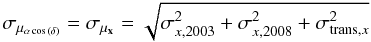 (B.1)and
 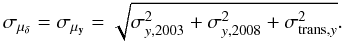 (B.2)The uncertainties of the position in the x- (east-west) and y-direction (north-south) in the proper motion plane (see Fig. 6) are denoted as σx, year and σy, year, respectively, and are the standard errors of the three independent measurements of the position of each star in the three auxiliary images (see Sect. 3.4). The residual rms deviations in the x- and y-direction of the geometric transformation, which is used to map the positions of the 2003 epoch onto the correct positions of the 2008 epoch, are σtrans, x and σtrans, y.
The proper motion membership criterion is derived from the total proper motion 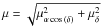 (see Sect. 5.3). The uncertainty of the combined proper motion σμ is therefore
  (B.3)where the astrometric uncertainty σpos,year is the average of the positional uncertainties in the x- and y-direction,
  (B.4)(see Sect. 3.4).
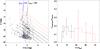 |
Fig. B.1 Left panel: colour–magnitude diagram of stars classified as belonging to the field according to their proper motion (dots) and of stars removed from the member sample based on their colour or known spectral type (triangles). Field stars which could only be discerned due to the knowledge of their spectral type are additionally drawn as diamonds. The vertical, short-dashed line and the second isochrone (AKs, cut = 2.89 mag, long-dashed line) indicate the position of the blue and the red colour-cut (see Sect. 6). The tilted lines, equally spaced in H-band, are lines of reddening according to the extinction law of Nishiyama et al. (2009) and are the boundaries of the bins used to estimate the residual contamination of the member sample. The estimation was performed in two different ways for bins 1 to 3 (counted from bottom to top, solid lines) and for bins 4 to 6 (dashed lines). Right panel: ratio of the number of expected contaminating field stars in the member sample after proper motion selection and colour-cut to the number of cluster members for the respective mass bin (see right panel) plotted vs. the initial mass as determined from the 4 Myr Padova isochrone. The number of contaminating field stars for the first three bins (solid) and for the bins 4 to 6 (dashed) are estimated according to Appendix C.2 and Appendix C.1, respectively. |
Appendix C: Assessment of the remaining contaminants in the cluster sample
After the proper motion member selection and the additional colour-cut had been applied (see Sect. 6), 6 M, K supergiants remained in the cluster sample and could only be removed because their spectral type is known from the LHO catalogue. In order to study the influence of hidden field stars in the final cluster sample on the MF slope, their number was estimated in the mass range from 4.6 ≤ mPad,4Myr ≤ 40.0 M⊙. The minimum mass of 4.6 M⊙ corresponds to the minimum mass entering the mass function for the 4 Myr Padova isochrone, while the upper mass boundary at mPad,4 Myr = 40.0 M⊙ is chosen such that for all stars with higher masses the spectral type is known and the final cluster sample can be considered clean. This mass range was splitted in six mass bins with equal spacing in H-band (see left panel in Fig. B.1, tilted lines). About 70% of all cluster members residing within the three uppermost bins (bins 4 to 6 in Table C.1, mPad,4 Myr ≥ 18.0 M⊙) have a unique counterpart in the LHO spectral catalogue (see Fig. 9). The estimation of the number of contaminating field stars ncont among stars without a spectral classification within bin 4 to 6 can therefore be based on the known number of M, K giants in each bin (Appendix C.1). Due to the lack of spectral identifications in the mass range mPad,4Myr < 18.0 M⊙ this is not possible for the bins 1 to 3. The assessment of ncont within these bins relies on the ratio of the number of field stars which are removed due to their red colour to the number of field stars identified by their proper motions in the same colour-range (see Appendix C.2). The MF slope is then re-determined after randomly selecting and removing the estimated number of contaminants within each mass bin from the final cluster sample (Appendix C.3).
Estimated remaining contaminations in the cluster member sample after proper motion and colour selection.
C.1. Estimation of ncont for mPad,4Myr ≥ 18.0 M⊙
50 stars out of a total of 568 stars in the final cluster sample have a unique counterpart of spectral type O or B in the LHO catalogue. Further 13 stars can not be assigned unambiguously to early type sources in the spectral catalogue. The ambiguous assignments for these stars are caused by the higher resolution of the NACO datasets such that several stars in the final catalogue are the potential counterparts of one source in the LHO catalogue (these stars are marked by an X-cross in Fig. 9). For the bulk of cluster members within the high mass bins (4 to 6) the spectral types are known. The 6 M, K supergiants, which were excluded from the final cluster sample, are located in the same region of the CMD. Therefore, the estimation of the number of contaminants among the stars without known spectral type can be based on the ratio of the number of known M, K supergiants nM, K to the number of spectroscopically classified early type stars nST (ST stands for spectral type) in the respective bin.
For each of the bins 4 to 6 the numbers of stars in the final cluster sample with a unique (nST), an ambiguous (nambST) and without assignment (nnoST) to a source in the LHO catalogue are determined. The number of stars with an ambiguous assignment within each bin is distributed among nST and nnoST. For example two stars in bin 6 are potential counterparts for the WR-star with number 47 in the LHO catalogue. As only one of the two stars is the true counterpart, nST and nnoST are both increased by one. If the two stars would reside in two different bins, nST and nnoST would be each increased by 0.5 in both bins.
The number of hidden M, K supergiants (ncont,MK) among the stars of the final cluster sample without or with ambiguous spectral identification within the bins 4 to 6 is the ratio of the number of identified M, K giants (nM,K) in the respective bin (see left panel in Fig. B.1) to nST times nnoST:  (C.1)These numbers are stated in Table C.1.
C.2. Estimation of ncont for mPad,4Myr < 18.0 M⊙
For stars fainter than about H = 15.5 mag the cluster membership of a star in the final cluster sample could not be confirmed by its spectral identification in the LHO catalogue anymore (see Fig. 9) and the number of residual field stars hidden in the final cluster sample can only be estimated. The estimation of ncont for stars with mPad,4Myr < 18.0 M⊙ uses the field stars outside the colour-cuts (see Fig. B.1, black triangles), to assess the ratio of the number of field stars, which are removed from the cluster sample solely due to their colour, to the number of field stars, which are already identified because of their proper motions. The field stars removed by the blue and the red colour-cut (see Sect. 6) belong to different populations, though.
Stars with colours H − Ks ≤ 1.3 are likely main sequence foreground stars located in the Galactic spiral arms. As these stars are co-moving with the disc with ~200 km s-1 and hence posses similar proper motions as the cluster, it is not possible to discriminate these stars based on their proper motion alone. However, they are very effectively removed by the blue colour-cut, as their colours due to their smaller distance and, therefore, lower extinction differ from the colour of stars in the inner bulge. In fact, for the mass bins 1 and 2 the number of presumed foreground stars, which are rejected because of their blue colour, is equal to or exceeds the number of blue proper motion non-members by a factor of five. At least for the lowermost mass bin cluster and foreground stars are more effectively discerned based on their colours than on their proper motions, which significantly increases the estimated number of contaminants for the respective mass bins. But because of the distinct colour ranges of stars in the final cluster sample and blue foreground stars from the spiral arms in the mass range used for the PDMF derivation (see Fig. 8), a significant contribution of foreground stars to the residual contamination of the final cluster sample is not expected. Therefore stars left of the blue colour-cut are not used to estimate the remaining contamination, as this would overestimate the number of contaminants.
Otherwise, the bulk of stars located in the Galactic bulge experience a similar or larger extinction as the cluster (see right panel in Fig. 8). Bulge stars, which due to their large number constitute the dominant source of contaminants for lines of sight towards the GC, are hence harder to discern from the cluster by their colour, but because of their randomized motion and systematically lower velocities (see Fig. 3 in Rich et al. 2007) they are more easily removed by the proper motion membership criterion.
To estimate the number of residual contaminants in the cluster sample for bins 1 to 3 we therefore use the red sources in the field star CMD. Within each of the mass bins 1 to 3, the number of field stars removed based on the red colour-cut (nf,red,cc) is divided by the number of field stars in the same colour-range identified by their proper motion (nf,red,pm). This ratio is then multiplied with the number of field stars between the red and blue colour-cut in that mass bin (nf,within cc) to retrieve the expected number of contaminating field stars in the cluster sample:  (C.2)The estimated numbers of contaminants ncont within the three mass bins are stated in Table C.1 (bin number 1 to 3).
The ratio of ncont to the number of cluster members nm (including the 6 known M, K supergiants) is drawn in Fig. B.1 (right panel) for all mass bins (solid for bins 1 to 3, dashed for bins 4 to 6). As for bins 1 to 3 ncont refers to the total number of contaminants after proper motion and colour-selection, the number of identified M, K supergiants nM,K is added to the estimated number of hidden field stars ncont for the bins 4 to 6. The error bars follow from error propagation assuming Poisson errors for the number of identified M, K supergiants and cluster members in each mass bin. The ratios ncont/nm are consistent for all mass bins within the uncertainties, with an expected average residual contamination of ⟨ ncont/nm ⟩ = 14 ± 5%.
As explained above we expect to overestimate ncont if stars left of the blue colour-cut are as well taken into account for the derivation of ncont, but we state the retrieved values for completeness. The usage of red and blue sources leads to considerably larger values of ncont for the mass bins 1 and 2, yielding 25.1 ± 10.4 and 9.8 ± 4.3 , respectively (see Table C.1 for comparison). The ratio ncont/nm for these two bins is raised to 0.23 ± 0.10 (bin 1) and 0.21 ± 0.10 (bin 2), which slightly increases the average residual contamination: ⟨ ncont/nm ⟩ = 16 ± 5%.
C.3. Influence of hidden field stars on the mass function slope
The influence of the contaminants on the mass function slope was studied for the mass function derived for the 4 Myr Padova isochrone. Within each mass bin, ncont stars, with ncont being the estimated number of contaminants in the respective mass bin, were randomly selected and removed from the final cluster sample. For the bins 4 to 6 only stars without spectral identification were selected and removed, whereas at least one star of each LHO number occurring in the full final cluster sample remained in the cluster sample. The mass function was then derived in the same way as for the full sample (see Sect. 8) using equal number bins (Method A).
To account for the error of ncont, the removed number of contaminants in each bin was independently varied between the three values ncont − Δncont, ncont and ncont + Δncont. For each combination of the removed number of contaminants per bin the random selection and removal of stars was repeated 100 times. The retrieved mass functions slopes α vary in the range between − 1.74 and − 1.50. The mean value of all derived slopes is − 1.63, which is the same slope as derived using the best value of ncont for all bins. In general the mass function slope flattens for a larger total number of removed stars, as the number of estimated contaminants (and the respective errors) increases towards lower masses. The steepest slopes are naturally derived for combinations where the ratio of the number of stars removed in bins 1 to 3 to the number of stars removed in bin 4 to 6 is largest. The steepest retrieved slope of − 1.74 ± 0.09 is still well contained within the errors of the MF slope for the 4 Myr Padova isochrone derived without accounting for residual field stars (α = −1.68 ± 0.09). On the other hand, the flattest slope − 1.50 ± 0.09 is considerably flatter, although the ranges of the formal fitting errors still marginally overlap. The mass function slopes reported in Table 5 can therefore (within the uncertainties) be regarded as lower (steep) limits for the true PDMF slope of the Quintuplet cluster.
If stars left of the blue colour-cut are considered during the estimation of ncont (see last paragraph of Appendix C.2), the
number of stars to be removed from the two lowest mass bins (bin 1 and 2) is significantly increased. The retrieved PDMF slopes are therefore flatter, ranging from α = −1.71 to −1.39 with an average value of α = −1.55 (compared to αmin = −1.74, αmax = −1.50 and a mean value of α = −1.63).
PyRAF is a product of the Space Telescope Science Institute, which is operated by AURA for NASA.
IRAF is distributed by the National Optical Astronomy Observatory, which is operated by the Association of Universities for Research in Astronomy (AURA) under cooperative agreement with the National Science Foundation.
Stars, whose peak flux exceeds the linearity limit of the detector are referred to as saturated stars for the remainder of this paper.
Carpenter (2003), see http://www.astro.caltech.edu/~jmc/2mass/v3/transformations/
Solar metallicity for the Geneva isochrone: X = 0.68, Y = 0.3, Z = 0.020 (Lejeune & Schaerer 2001); solar metallicity for the Padova isochrones: X = 0.708, Y = 0.273, Z = 0.019 for M < 7 M⊙ (Marigo et al. 2008; Girardi et al. 2000), X = 0.7, Y = 0.28, Z = 0.020 for M > 7 M⊙ (Bertelli et al. 1994; Bressan et al. 1993).
Acknowledgments
The authors would like to thank the supportive, anonymous referee for helpful comments and suggestions. We also thank P. Lucas for his support with the calibration of our data vs. UKDISS. We are much obliged to the NAOS-CONICA instrument scientist team for their careful observations in Service Mode. B.H. and A.S acknowledge funding by the German Science Foundation (DFG) Emmy Noether Programme under grant STO 496/3-1.
References
- Ageorges, N., Lidman, C., Kaufer, A., & Hainaut, O. 2007, Very Large Telescope NAOS-CONICA User Manual, 81st edn. (Garching: ESO) [Google Scholar]
- Alves, D. R. 2000, ApJ, 539, 732 [NASA ADS] [CrossRef] [MathSciNet] [Google Scholar]
- Bertelli, G., Bressan, A., Chiosi, C., Fagotto, F., & Nasi, E. 1994, A&AS, 106, 275 [NASA ADS] [Google Scholar]
- Bessell, M. S., & Brett, J. M. 1988, PASP, 100, 1134 [NASA ADS] [CrossRef] [Google Scholar]
- Brandner, W., Clark, J. S., Stolte, A., et al. 2008, A&A, 478, 137 [NASA ADS] [CrossRef] [EDP Sciences] [Google Scholar]
- Bressan, A., Fagotto, F., Bertelli, G., & Chiosi, C. 1993, A&AS, 100, 647 [NASA ADS] [Google Scholar]
- Carpenter, J. M. 2001, AJ, 121, 2851 [NASA ADS] [CrossRef] [Google Scholar]
- Da Rio, N., Gouliermis, D. A., & Henning, T. 2009, ApJ, 696, 528 [NASA ADS] [CrossRef] [Google Scholar]
- Degl’Innocenti, S., Prada Moroni, P. G., Marconi, M., & Ruoppo, A. 2008, Ap&SS, 316, 25 [NASA ADS] [CrossRef] [Google Scholar]
- Devillard, N. 2001, in Astronomical Data Analysis Software and Systems X, ed. F. R. Harnden Jr., F. A. Primini, & H. E. Payne (San Francisco: ASP), ASP Conf. Ser., 238, 525 [Google Scholar]
- Diolaiti, E., Bendinelli, O., Bonaccini, D., et al. 2000, A&AS, 147, 335 [NASA ADS] [CrossRef] [EDP Sciences] [Google Scholar]
- Eisenhauer, F., Quirrenbach, A., Zinnecker, H., & Genzel, R. 1998, ApJ, 498, 278 [NASA ADS] [CrossRef] [Google Scholar]
- Espinoza, P., Selman, F. J., & Melnick, J. 2009, A&A, 501, 563 [NASA ADS] [CrossRef] [EDP Sciences] [Google Scholar]
- Figer, D. F. 2008, in Massive Stars as Cosmic Engines, ed. F. Bresolin, P. A. Crowther, & J. Puls (Cambridge: Cambridge Univ. Press), Proc. IAU Symp., 250, 247 [Google Scholar]
- Figer, D. F., McLean, I. S., & Morris, M. 1995, ApJ, 447, L29 [NASA ADS] [CrossRef] [Google Scholar]
- Figer, D. F., Najarro, F., Morris, M., et al. 1998, ApJ, 506, 384 [NASA ADS] [CrossRef] [Google Scholar]
- Figer, D. F., Kim, S. S., Morris, M., et al. 1999a, ApJ, 525, 750 [NASA ADS] [CrossRef] [Google Scholar]
- Figer, D. F., McLean, I. S., & Morris, M. 1999b, ApJ, 514, 202 [NASA ADS] [CrossRef] [Google Scholar]
- Fruchter, A., & Hook, R. 2002, PASP, 114, 144 [NASA ADS] [CrossRef] [Google Scholar]
- Gennaro, M., Brandner, W., Stolte, A., & Henning, T. 2011, MNRAS, 412, 2469 [NASA ADS] [CrossRef] [MathSciNet] [Google Scholar]
- Ghez, A. M., Salim, S., Weinberg, N. N., et al. 2008, ApJ, 689, 1044 [NASA ADS] [CrossRef] [Google Scholar]
- Girardi, L., Bressan, A., Bertelli, G., & Chiosi, C. 2000, A&AS, 141, 371 [NASA ADS] [CrossRef] [EDP Sciences] [Google Scholar]
- Glass, I. S., Moneti, A., & Moorwood, A. F. M. 1990, MNRAS, 242, 55 [Google Scholar]
- Hambly, N. C., Collins, R. S., Cross, N. J. G., et al. 2008, MNRAS, 384, 637 [NASA ADS] [CrossRef] [Google Scholar]
- Harayama, Y., Eisenhauer, F., & Martins, F. 2008, ApJ, 675, 1319 [NASA ADS] [CrossRef] [Google Scholar]
- Hodgkin, S. T., Irwin, M. J., Hewett, P. C., & Warren, S. J. 2009, MNRAS, 394, 675 [NASA ADS] [CrossRef] [Google Scholar]
- Kim, S. S., Figer, D. F., Lee, H. M., & Morris, M. 2000, ApJ, 545, 301 [NASA ADS] [CrossRef] [Google Scholar]
- Kim, S. S., Figer, D. F., Kudritzki, R. P., & Najarro, F. 2006, ApJ, 653, L113 [NASA ADS] [CrossRef] [Google Scholar]
- Kobayashi, Y., Okuda, H., Sato, S., Jugaku, J., & Dyck, H. M. 1983, PASJ, 35, 101 [NASA ADS] [Google Scholar]
- Kroupa, P. 2001, MNRAS, 322, 231 [NASA ADS] [CrossRef] [Google Scholar]
- Lawrence, A., Warren, S. J., Almaini, O., et al. 2007, MNRAS, 379, 1599 [NASA ADS] [CrossRef] [MathSciNet] [Google Scholar]
- Lejeune, T., & Schaerer, D. 2001, A&A, 366, 538 [NASA ADS] [CrossRef] [EDP Sciences] [Google Scholar]
- Lenzen, R., Hartung, M., Brandner, W., et al. 2003, in SPIE Conf. Ser. 4841, ed. M. Iye, & A. F. M. Moorwood, 944 [Google Scholar]
- Liermann, A., Hamann, W.-R., & Oskinova, L. M. 2009, A&A, 494, 1137 [NASA ADS] [CrossRef] [EDP Sciences] [Google Scholar]
- Liermann, A., Hamann, W.-R., Oskinova, L. M., Todt, H., & Butler, K. 2010, A&A, 524, A82 [NASA ADS] [CrossRef] [EDP Sciences] [Google Scholar]
- Lu, J. R., Ghez, A. M., Hornstein, S. D., et al. 2009, ApJ, 690, 1463 [NASA ADS] [CrossRef] [Google Scholar]
- Lucas, P. W., Hoare, M. G., Longmore, A., et al. 2008, MNRAS, 391, 136 [NASA ADS] [CrossRef] [Google Scholar]
- Lundin, L. K., Ballester, P., & Peron, M. 2007, Very Large Telescope NACO Pipeline User Manual (Garching: ESO) [Google Scholar]
- Maíz Apellániz, J., & Úbeda, L. 2005, ApJ, 629, 873 [NASA ADS] [CrossRef] [Google Scholar]
- Marigo, P., Girardi, L., Bressan, A., et al. 2008, A&A, 482, 883 [NASA ADS] [CrossRef] [EDP Sciences] [Google Scholar]
- Mauerhan, J. C., Cotera, A., Dong, H., et al. 2010a, ApJ, 725, 188 [NASA ADS] [CrossRef] [Google Scholar]
- Mauerhan, J. C., Muno, M. P., Morris, M. R., Stolovy, S. R., & Cotera, A. 2010b, ApJ, 710, 706 [NASA ADS] [CrossRef] [Google Scholar]
- Meynet, G., Maeder, A., Schaller, G., Schaerer, D., & Charbonnel, C. 1994, A&AS, 103, 97 [NASA ADS] [Google Scholar]
- Morris, M. 1993, ApJ, 408, 496 [NASA ADS] [CrossRef] [Google Scholar]
- Morris, M., & Serabyn, E. 1996, ARA&A, 34, 645 [NASA ADS] [CrossRef] [Google Scholar]
- Nagata, T., Woodward, C. E., Shure, M., Pipher, J. L., & Okuda, H. 1990, ApJ, 351, 83 [NASA ADS] [CrossRef] [Google Scholar]
- Najarro, F., Figer, D. F., Hillier, D. J., & Kudritzki, R. P. 2004, ApJ, 611, L105 [NASA ADS] [CrossRef] [Google Scholar]
- Nishiyama, S., Nagata, T., Sato, S., et al. 2006, ApJ, 647, 1093 [NASA ADS] [CrossRef] [Google Scholar]
- Nishiyama, S., Tamura, M., Hatano, H., et al. 2009, ApJ, 696, 1407 [NASA ADS] [CrossRef] [Google Scholar]
- Okuda, H., Shibai, H., Nakagawa, T., et al. 1990, ApJ, 351, 89 [NASA ADS] [CrossRef] [Google Scholar]
- Portegies Zwart, S. F., Makino, J., McMillan, S. L. W., & Hut, P. 2002, ApJ, 565, 265 [NASA ADS] [CrossRef] [Google Scholar]
- Rich, R. M., Reitzel, D. B., Howard, C. D., & Zhao, H. 2007, ApJ, 658, L29 [NASA ADS] [CrossRef] [Google Scholar]
- Rousset, G., Lacombe, F., Puget, P., et al. 2003, in SPIE Conf. Ser. 4839, ed. P. L. Wizinowich, & D. Bonaccini, 140 [Google Scholar]
- Salpeter, E. E. 1955, ApJ, 121, 161 [Google Scholar]
- Schaller, G., Schaerer, D., Meynet, G., & Maeder, A. 1992, A&AS, 96, 269 [Google Scholar]
- Schödel, R., Najarro, F., Muzic, K., & Eckart, A. 2010, A&A, 511, A18 [NASA ADS] [CrossRef] [EDP Sciences] [Google Scholar]
- Skrutskie, M. F., Cutri, R. M., Stiening, R., et al. 2006, AJ, 131, 1163 [NASA ADS] [CrossRef] [Google Scholar]
- Stolte, A., Grebel, E. K., Brandner, W., & Figer, D. F. 2002, A&A, 394, 459 [NASA ADS] [CrossRef] [EDP Sciences] [Google Scholar]
- Stolte, A., Ghez, A. M., Morris, M., et al. 2008, ApJ, 675, 1278 [NASA ADS] [CrossRef] [Google Scholar]
- Straižys, V., & Laugalys, V. 2008, Baltic Astron., 17, 253 [NASA ADS] [Google Scholar]
- van der Hucht, K. A. 2006, A&A, 458, 453 [NASA ADS] [CrossRef] [EDP Sciences] [Google Scholar]
- Weidner, C., Kroupa, P., & Maschberger, T. 2009, MNRAS, 393, 663 [NASA ADS] [CrossRef] [Google Scholar]
- Yungelson, L. R., van den Heuvel, E. P. J., Vink, J. S., Portegies Zwart, S. F., & de Koter, A. 2008, A&A, 477, 223 [NASA ADS] [CrossRef] [EDP Sciences] [Google Scholar]
All Tables
Catalogue of stellar sources with measured proper motions and colours in the Quintuplet cluster.
Overview of derived slopes of the mass function binning the data into 12 bins containing approximately the same number of stars.
Comparison of mass function slopes in the centres of Galactic young massive clusters.
Estimated remaining contaminations in the cluster member sample after proper motion and colour selection.
All Figures
|
Fig. 1 VLT NACO JHKs composite image of the Quintuplet cluster. Outside the dotted rectangle only H- and Ks-band data are available. The dashed circle with a radius of 500 pixel or 0.5 pc indicates the region used for the derivation of the mass function (see Sect. 5.2). Due to bad AO correction, the J-band dataset was unsuitable to perform photometry and astrometry and was used only for this composite image. |
| In the text | |
|
Fig. 2 Plot of the astrometric uncertainty (left panels) and the photometric uncertainty (right panels) vs. the magnitude for all four NACO datasets. The plotted photometric uncertainty does only include the PSF fitting uncertainty. The dashed lines mark the linearity limit of the respective dataset. |
| In the text | |
|
Fig. 3 Difference of the inserted and recovered magnitudes of artificial stars inserted into the combined image of the Ks-band data in 2008 plotted vs. the magnitude. A high-order polynomial fit to the median and the standard deviation (multiplied by a factor of 1.5) of the magnitude difference within magnitude bins of 1 mag are shown as well. The vertical dotted line indicates the maximum Ks-band magnitude at Ks = 19 mag of stars to be used for the proper motion analysis. |
| In the text | |
|
Fig. 4 Left panel: recovery fractions of artificial stars inserted within the inner 500 pixel from the centre of the observed field plotted vs. the respective magnitude in the Ks- (lower abscissa) or H-band (upper abscissa). The full and dotted lines correspond to the recovery fractions for the Ks-band data in 2003 and 2008, respectively and the dash-dotted line shows the completeness in the H-band. The dashed line shows the total completeness for the stars after matching the two Ks-band and the H-band datasets. Only stars with Ks < 19 mag are used for the proper motion analysis, as indicated by the vertical dotted line. Right panel: Ks-band image from the second epoch with the overplotted contours representing a completeness level of 50% for the labelled magnitudes. |
| In the text | |
|
Fig. 5 Left panel: plot of the combined astrometric uncertainty from the two epochs of Ks-band data plotted vs. the magnitude of the second epoch (for details of the error estimation see Sect. 3.4). The median and standard deviation of the astrometric uncertainty above the linearity limit (at 14.3 mag) of the dataset in 2003 with 20.0 s DIT were fitted by polynomials. This fit of the median (lower line) and the sum the median and standard deviation (upper line) are drawn in all three plots. Middle panel: astrometric uncertainty of stars residing within a circle with |
| In the text | |
|
Fig. 6 Proper motion diagram of stars with Ks ≤ 19 mag. The dashed line marks the direction parallel to the Galactic plane, the dotted line is oriented vertically with respect to the Galactic plane and splits the proper motion diagram into the north-east and the south-west segment. Stars within a radius of 2σ as derived from the Gaussian fit in Fig. 7 (right panel) around the origin are selected as cluster members. |
| In the text | |
|
Fig. 7 Left panel: histogram of proper motions parallel to the Galactic plane. Middle panel: histogram of proper motions vertical to the Galactic plane. Right panel: histogram of the 2-dimensional proper motions located in the north-east-segment of the proper motion diagram. The histogram was fitted with a Gaussian function and a 2σ cut was used as the selection criterion for cluster membership (dash-dotted lines in all three panels). |
| In the text | |
|
Fig. 8 Left panel: colour–magnitude diagram of cluster member candidates on the basis of their proper motions. A 4 Myr isochrone with solar metallicity, combined using a Padova MS-isochrone and a Pisa-FRANEC PMS-isochrone, shifted to a distance of 8 kpc and a foreground extinction of AKs = 2.35 mag, is shown for reference. Stars, with fluxes exceeding the linearity limit of the detector are drawn as crosses in all figures throughout this paper. A two-step colour-cut was applied for stars with H > 14 mag to remove field stars with similar proper motions as the cluster from the cluster sample (see Sect. 6 for details). The vertical short-dashed lines mark the first colour-cut, while in the second step of the colour-cut highly reddened objects to the right of the second isochrone (AKs = 2.89 mag, long-dashed line) are removed. The dots represent the sample of cluster stars after the colour-cut, stars rejected based on their colour are drawn as triangles. Spectroscopically identified field supergiants from the LHO catalogue (Liermann et al. 2009) are marked with diamonds and are removed from the final cluster sample. Right panel: colour–magnitude diagram of stars classified as belonging to the field according to their proper motion (dots) and of stars removed from the member sample based on their colour or known spectral type (triangles). One star, classified as belonging to the field by its proper motion, has an O-star as (ambiguous) counterpart in the LHO catalogue (see Sect. 6) and is marked with a circle. The tilted dotted line is the line of reddening according to the extinction law by Nishiyama et al. (2009) running through the population of red clump stars from the Galactic bulge. |
| In the text | |
|
Fig. 9 Colour–magnitude diagram of the final cluster sample. Stars with counterparts in the LHO catalogue are flagged with symbols according to their spectral type (box: WR-stars, circle: OB-stars, stars with ambiguous identification are additionally marked with an X-cross). The horizontal dashed and short-dashed lines mark the initial masses along the isochrone in units of M⊙. The tilted dotted lines show the lines of reddening according to the extinction law by Nishiyama et al. (2009) and enframe the two regions in the CMD (shaded in grey in Figs. 9–11), within which the isochrone has multiple intersections with the line of reddening, and consequently no unique mass can be inferred for a given star. |
| In the text | |
|
Fig. 10 Colour–magnitude diagram of all stars of the final cluster sample with proper motions residing in the north-east (left panel) or south-west segment (right panel) of the proper motion diagram (Fig. 6). See Figs. 8 and 9 for details. |
| In the text | |
|
Fig. 11 Comparison of the four isochrones used to determine stellar masses. For all shown isochrones, solar metallicity, a distance to the cluster of 8 kpc and a foreground extinction of AKs = 2.35 mag is adopted. As in Figs. 9 and 10, the dotted lines enframe regions in the CMD with ambiguous mass assignments (shaded in grey) and the initial masses are labelled along the isochrones. |
| In the text | |
|
Fig. 12 Comparison of the mass function and derived slopes for different methods of binning the data and performing the linear fit. Only the fit and derived slope for the completeness corrected mass function are shown. Left panel: mass function of the Quintuplet cluster with initial masses derived from the 4 Myr Padova isochrone. Only stars with m > 4.6 M⊙, i.e. stars above the ambiguity region in the CMD due to the PMS, are used. Wolf-Rayet stars are not included in the mass function, as the large uncertainty of their mass might bias the derived slopes. The bin sizes are adjusted such that each of the 12 bins holds approximately the same number of stars. Right panel: mass function of the same data but distributing the stars into 12 bins of a uniform logarithmic width of 0.084 dex adopting the same lower and upper mass limits as in the left panel. The solid line shows the weighted linear fit, the dotted line the unweighted fit. |
| In the text | |
|
Fig. 13 Upper panels: mass functions for the 4 Myr MS-Padova isochrone using all stars (left), or only stars located in the north-east- (middle), or south-west-segment (right) of the proper motion diagram (Fig. 6). Lower panels: resulting mass function if stellar masses are derived from a 3 or 5 Myr Padova MS-isochrone (left and middle) or 4 Myr Geneva isochrone (right). For all shown mass functions the stars were distributed in 12 bins of variable width with equal numbers of stars per bin. As in Fig. 12, the Wolf-Rayet stars were removed and only stars above the ambiguity region in the CMD due to the PMS are included. The resulting minimum masses are 5.5, 4.6, 4.0, and 4.5 M⊙, for the 3, 4, 5 Myr Padova and the 4 Myr Geneva isochrone, respectively. |
| In the text | |
|
Fig. B.1 Left panel: colour–magnitude diagram of stars classified as belonging to the field according to their proper motion (dots) and of stars removed from the member sample based on their colour or known spectral type (triangles). Field stars which could only be discerned due to the knowledge of their spectral type are additionally drawn as diamonds. The vertical, short-dashed line and the second isochrone (AKs, cut = 2.89 mag, long-dashed line) indicate the position of the blue and the red colour-cut (see Sect. 6). The tilted lines, equally spaced in H-band, are lines of reddening according to the extinction law of Nishiyama et al. (2009) and are the boundaries of the bins used to estimate the residual contamination of the member sample. The estimation was performed in two different ways for bins 1 to 3 (counted from bottom to top, solid lines) and for bins 4 to 6 (dashed lines). Right panel: ratio of the number of expected contaminating field stars in the member sample after proper motion selection and colour-cut to the number of cluster members for the respective mass bin (see right panel) plotted vs. the initial mass as determined from the 4 Myr Padova isochrone. The number of contaminating field stars for the first three bins (solid) and for the bins 4 to 6 (dashed) are estimated according to Appendix C.2 and Appendix C.1, respectively. |
| In the text | |
Current usage metrics show cumulative count of Article Views (full-text article views including HTML views, PDF and ePub downloads, according to the available data) and Abstracts Views on Vision4Press platform.
Data correspond to usage on the plateform after 2015. The current usage metrics is available 48-96 hours after online publication and is updated daily on week days.
Initial download of the metrics may take a while.