| Issue |
A&A
Volume 540, April 2012
|
|
|---|---|---|
| Article Number | A67 | |
| Number of page(s) | 6 | |
| Section | Astrophysical processes | |
| DOI | https://doi.org/10.1051/0004-6361/201117501 | |
| Published online | 27 March 2012 | |
Determining gravitational wave radiation from close galaxy pairs using a binary population synthesis approach
1 National Astronomical Observatories/Xinjiang Observatory, Chinese Academy of Sciences, 150 Science 1-Street Urumqi, 830011 Xinjiang, PR China
e-mail: This email address is being protected from spambots. You need JavaScript enabled to view it.
2 National Astronomical Observatories/Yunnan Observatory, Chinese Academy of Sciences, 650011 Kunming, PR China
3 Graduate University of the Chinese Academy of Sciences, 100049 Beijing, PR China
Received: 17 June 2011
Accepted: 17 February 2012
Abstract
Context. The early phase of the coalescence of supermassive black hole (SMBH) binaries from their host galaxies provides a guaranteed source of low-frequency (nHz − μHz) gravitational wave (GW) radiation by pulsar timing observations. These types of GW sources would survive the coalescing and be potentially identifiable.
Aims. We aim to provide an outline of a new method for detecting GW radiation from individual SMBH systems based on the Sloan Digital Sky Survey (SDSS) observational results, which can be verified by future observations.
Methods. Combining the sensitivity of the international Pulsar Timing Array (PTA) and the Square Kilometer Array (SKA) detectors, we used a binary population synthesis (BPS) approach to determine GW radiation from close galaxy pairs under the assumption that SMBHs formed at the core of merged galaxies. We also performed second post-Newtonian approximation methods to estimate the variation of the strain amplitude with time.
Results. We find that the value of the strain amplitude h varies from about 10-14 to 10-17 using the observations of 20 years, and we estimate that about 100 SMBH sources can be detected with the SKA detector.
Key words: binaries: general / black hole physics / stars: evolution / gravitational waves
© ESO, 2012
1. Introduction
A gravitational wave (GW), which is described as a space perturbation of the metric traveling at the speed of light, is a natural consequence of Einstein’s theory of gravity (“general relativity”, Einstein 1916, 1918). It has been accepted (Thorne & Braginskii 1976) that supermassive black hole (SMBH) binaries, which are ubiquitous in the nuclei of low-redshift galaxies (Magorrian et al. 1998), are bona fide GW sources, which can be detected with the international Pulsar Timing Array (PTA) and the proposed Square Kilometer Array (SKA) (Detweiler 1979; Hellings & Downs 1983; Kaspi et al. 1994; Wyithe & Loeb 2003; Jenet et al. 2005; Yardley et al. 2010). The precision of the rotation periods for millisecond period pulsars, which is established via pulse arrival time measurements, allows the detection of stochastic SMBH GW background spectrum at nHz frequencies (Rajagopal & Romani 1995; Jenet et al. 2006). These observations give us a good prospect for detecting GWs from the ensemble of these SMBH coalescence events throughout the universe. Some of these studies have been taken up by other groups over the years. In particular, the sensitivity curve of the SKA to GWs emitted by SMBH systems has been obtained from 100 pulsars using the Australia Telescope National Facility pulsar catalog (Yardley et al. 2010).
The frequent growth of galaxies by merger processes and SMBH in galaxies result in some obvious mechanisms about the formation of SMBHs. Several studies have argued that an occupation fraction of SMBH as low as 0.01 at reshift 5 can be obtained from subsequent mergers (Menou et al. 2001, and references therein). Spherical galaxies often lead to coalescence timescales that are longer than the Hubble time, while highly flattened or triaxial galaxies lead to faster coalescence (Wyithe & Loeb 2003). Therefore this expected GW radiation investigation from coalescing SMBHs depends on the merger rate of massive galaxies, the demographics of SMBHs at low- and high- redshift, and the dynamics of SMBH binaries. Meanwhile the SMBHs need to reach a regime where GW radiation can drive the main evolutionary process (Begelman et al. 1980). If the galaxy pairs can evolve to this GW radiation regime, they will gradually lose angular momentum to GW radiation and will eventually coalescence. The emission of GWs from SMBH sources requires that the binary coalesce in less than the Hubble time.
Some results of close galaxy pairs have been released from the Sloan Digital Sky Survey (SDSS) data (Ellison et al. 2008, 2010), such as the star formation rate, the merger rate of massive galaxies, the demographics of SMBHs at low redshift (z < 0.1) and the dynamics of SMBHs. A binary population synthesis (BPS) approach has been applied to study the characteristics of clusters and galaxies (see, e.g., Han et al. 2007; Zhang et al. 2010). This method has also been systematically taken up by some groups to investigate the GW radiation from compact binaries in the Galaxy (Nelemans et al. 2001; Liu 2009; Liu et al. 2010; Ruiter et al. 2010). However, the GW radiation from SMBHs, combined with the BPS model and observation results, are not well known. Here we report how BPS, using SDSS results, can be used to determine the GW radiation from SMBHs.
In the next section, the binary population synthesis (BPS) model is described. In Sect. 3, we present the results of our simulations. And the discussion is given in Sect. 4.
2. The binary population synthesis model
2.1. Confirming the evolution trace of SMBH systems with OJ287
Supermassive black holes are expected to be a type of GW sources, but few studies can accurately determine a galaxy pair’s internal compositions and kinematics equations. The BL Lacertae object OJ287 (Sillanpaa et al. 1988, 1996; Valtonen 2007) provides a possible insight into the precessional elliptical orbital evolution through GW radiation in the phase of coalescence of SMBH binaries. The basic elements of this phase are as follows: 12-year intervals in optical outburst, component masses 1.3 × 10⁸ M⊙ and 1.8 × 10¹⁰ M⊙, an orbital period of nine years, an eccentricity of 0.67, a distance of 1.3 Gpc.
In accordance with Einstein’s general relativity, the metric can be written as
 (1)where ηαβ is Minkowsky metric, and hαβ stands for GWs with |hαβ| ≪ 1. The amplitude and the luminosity of GW radiation are
  (2)and
  (3)where G and c are the gravitational constant and speed of light, respectively. ℛ is the distance from the GW sources to the Earth, Dij is the polar moment of mass, and the symbol ⟨ ⟩ denotes the averaging.
The SMBHs move increasingly closer because of GW radiation over time, therefore the lifetime of galaxy pairs before the final in-spiral is (Jaffe & Backer 2003)  (4)where M8 stands for the total mass of the binary in units of 108 M⊙, q ( = m1/m2 < 1) is the mass ratio, Porb is the orbital period in years. Meanwhile, the orbital angular momentum loss from two point masses is given by
  (5)where r is the separation of SMBHs in the galaxy pairs.
As displayed above, an important quantity to be considered is the GW amplitude h, here we give a simple description of the calculation ofh in our simulations. First, we give the definition for the polar moment of mass Dij in Eq. (3)  (6)where
  , and i,j = 1,2. In general, we need to calculate this energy momentum tensor for an isolated system. For our particle binaries we just simulate the equation of motion of each BH using a numerical method. The primary of an SMBH system is defined here as the initially more massive component (m2) throughout. We also assumed that the primary BH m2 is at the origin of coordinate, and that the secondary BH m1( < m2) traces out the precessional elliptical orbit around this primary.
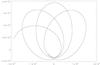 |
Fig. 1 Orbital trace template of SMBH systems using OJ287. The primary BH is at coordinates (0, 0). The precessional elliptical curve represents the evolutionary trace of the secondary BH. |
According to Eq. (16) of Antonacopoulos (1979), the equation of motion of the secondary m1 can be described as ![Mathematical equation: \begin{eqnarray} \frac{{\rm d} \bar{u}_{1}}{{\rm d}t}=-{G}\frac{m_{2}(\vec{x}_{1}-\vec{x}_{2})}{\mid \vec{x}_{1}-\vec{x}_{2}\mid ^{3}}\hspace{129pt}\nonumber \\+\frac{1}{{c^2}} \Bigg[-{G}\frac{m_{2}(\vec{x}_{1}-\vec{x}_{2})}{\mid \vec{x}_{1}-\vec{x}_{2}\mid ^{3}}\vec{u_{1}}^{2}+{4G}\frac{m_{2}(\vec{x}_{1}-\vec{x}_{2})\cdot \vec{u}_1}{\mid \vec{x}_{1}-\vec{x}_{2}\mid ^{3}}\vec{u}_1\nonumber\\+{4 G}^{2}\frac{m_{2}^{2}(\vec{x}_{1}-\vec{x}_{2})}{\mid \vec{x}_{1}-\vec{x}_{2}\mid ^{4}}\Bigg]+\frac{1}{{c^4}} \Bigg[-2{G}^{2}\frac{m_{2}^2(\vec{x}_{1}-\vec{x}_{2})\cdot \vec{u}_1}{\mid \vec{x}_{1}-\vec{x}_{2}\mid ^{4}}\vec{u_{1}}\nonumber\\ -{9 G}^3\frac{m_{2}^3(\vec{x}_{1}-\vec{x}_{2})}{\mid \vec{x}_{1}-\vec{x}_{2}\mid ^{5}}+{2 G}^{2}\frac{m_{2}^{2}[(\vec{x}_{1}-\vec{x}_{2})\cdot\vec{u}_{1}]^2}{\mid \vec{x}_{1}-\vec{x}_{2}\mid ^{6}}(\vec{x}_{1}-\vec{x}_{2})\Bigg], \end{eqnarray}](/articles/aa/full_html/2012/04/aa17501-11/aa17501-11-eq32.png) (7)where x1 and x2 are the vector position of secondary and primary in the BH binaries, respectively. And u1 is the vector velocity of secondary BH. To facilitate the calculation, we derive from Eq. (7) using the polar coordinate
(7)where x1 and x2 are the vector position of secondary and primary in the BH binaries, respectively. And u1 is the vector velocity of secondary BH. To facilitate the calculation, we derive from Eq. (7) using the polar coordinate 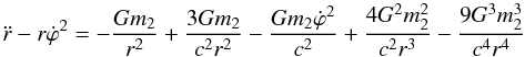 (8)
(8)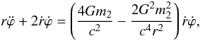 (9)here r = |x1 − x2|. Here we neglect the influence of the smaller quantity (such as
  ) in Eqs. (7) − (9). We did not perform the calculation in full relativity.
To fix the orbital trace of SMBHs, which is consistent with OJ 278’s modulation, we investigated the numerical result using the followed initial parameters of the position of periastron: r0 = 3162 AU, ϕ0 = 0, ṙ0 = 0 and the tangent components of the velocity v0 = 0.275c, the subscript 0 denotes the initial values. Therefore, Fig. 1 shows an orbital evolution trace of the secondary BH. Note that our calculation of the precessing-binary model is slightly different from that of Fig. 1 of Valtonen (2007), which is consistent with the fixed optical outbursts of OJ287 according to an accretion disk model. In other words, we excluded the influence of the accretion disk from our definition. That is mainly because the accretion disk dominates the electromagnetic radiation. Our simulations focus on the importance of GW radiation.
To analyze the GW amplitude over time, from Eq. (6), the components of the mass tensor (Capozziello et al. 2008) are 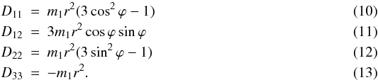 Here other quantities Dij = 0. The change of the GW amplitude is illustrated in Fig. 2. We can note four kinds of information from it. Firstly, we consider OJ287 as our standard template and obtain some typical feedback: the orbital period is 9.4 yr, the precessional motion is 40o per period, and the eccentricity is 0.71. Secondly, this numerical curve covers about 40 years from 1996 to 2036. And the maximum quantities of GW amplitude will appear on the position at which the secondary BH moves to the position of periastron. To some extent, we also find that the events that happened in maximum position are consistent with those of the optical outburst. For example, during 2005–2006 (Valtonen et al. 2008), the time of outburst from OJ287 is very close to a position of maximum GW radiation in our manifestation. In other words, if the OJ287 experiences an outburst in 2020, the very high possibility of GW detection can be investigated using pulsars around 2020. Thirdly, we find that the GW signal from this type of individual SMBH sources at the Earth is unlikely to be detected (the position of the symbol “today” is about 5 × 10-16 in 2012) using a current PTA detector, which agrees with estimates from previous studies (Hobbs et al. 2009; Sesana et al. 2009; Yardley et al. 2010). Finally, these descriptions of the GW are the crucial criteria that we adopt throughout.
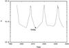 |
Fig. 2 Amplitude h as a function of the observation time for the OJ287’s model. The symbol “ ⋆ ” indicates the position at which the GW radiation from OJ287 is, ~5 × 10-16 in 2012. |
2.2. Parameters in the Monte Carlo simulation
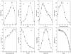 |
Fig. 3 Fitting physical property curves of Monte Carlo parameters are derived from SDSS (Ellison et al. 2010) in panels a)–g), whose error bars represent the uncertainties of estimation due to the fitting errors in galaxy pairs of SDSS. The BH mass function curve is also display in panel h), which is the same as that of Tamura et al. (2006). |
To systematically investigate the GW radiation of galaxy pair systems, we performed a Monte Carlo simulation through which we followed the evolution of a sample of 1 million binaries. The description of our input physics parameters is given as follows.
-
(i)
The properties of the overall galaxy pair samples have beendisplayed in the released SDSS data (Ellison et al.2010), including projected and angular separation, relativevelocities (Δυ), stellar mass ratio, and redshift. We present polynomial curve fitting formulae, which we used to construct the distribution function of galaxy pairs (see Figs. 1 and 2 of Ellison et al. 2010), which approximate the evolution of SMBHs for a wide range of mass M(108 − 1012 M⊙) and stellar environment log Σ( − 1.4 − 1.4 Mpc-2). In our Fig. 3 (see panels (a) − (g)) we give the fitting curves of the physical properties for the galaxy pair sample using these released SDSS data.
-
(ii)
The star formation rate (SFR) is taken to be constant in the simulation (Ellison et al. 2008).
-
(iii)
According to the derivation of the black hole mass function (BHMF) at low redshift (Tamura et al. 2006), a simple polynomial curve fitting approximation of BHMF is also used in panel (h) of Fig. 3.
-
(iv)
We assumed that the merger rate of nearby (z < 0.1) galaxy pairs is 0.2 yr-1 in the phase of coalescence with a chirp mass of 1010 M⊙.
To construct the SMBH systems, other parameters used in the typical SMBH binary formation in this work are given as follows.
- (i)
The correlation between the massMBH of the BH and the velocity dispersion σ is given by (Tremaine et al. 2002)
 (14)where σ0 = 200 km s-1, α = 8.13 and β = 4.02.
 - (ii)
For the BH mass and the luminosity relation, we adopted the B-band relation described by (Bell et al. 2004)
 (15)
(15) - (iii)
A gravitational potential in a galaxy includes the bulge, disk, and halo potentials. The disk and bulge potentials are derived from (Miyamoto & Nagai 1975)
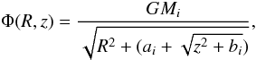 (16)where R and z are the galaxy center coordinate parameters and
  . The index i corresponds to bulge and disk. The halo potential is given as (Paczynski 1990)
 ![Mathematical equation: \begin{equation} \Phi (r)=-\frac{GM_{\rm c}}{r_{\rm c}}\left[\frac{1}{2}{\rm ln}\left(1+\frac{r^2}{r_{\rm c}^2}\right)+\frac{r_{\rm c}}{r}{\rm atan}\left(\frac{r}{r_{\rm c}}\right)\right]\cdot \end{equation}](/articles/aa/full_html/2012/04/aa17501-11/aa17501-11-eq70.png) (17)
(17)
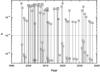 |
Fig. 4 Strain amplitude of GW radiation variation with time. The symbol “A” represents the average value position of the summed GW strain in each bin. The dotted line (log h = −15) marks the highest sensitivity of SKA. |
3. Results
With a BPS simulation we obtained a series of SMBHB systems from a sample of 1 million initial SMBHBs. Based on the sensitivity curves of the PTA and SKA detectors (Yardley et al. 2010), we created the time series for the source signals and added the individual time series of the calculated sources to produce the total data stream. Similar calculations of the GW signal analysis combined with a GW detector can be found in Sesana et al. (2008), Liu (2009), and Ruiter et al. (2010).
Figures 4 and 5 show the variation of the strain amplitude and luminosity with time from the GW radiation of SMBHs during a long time observation (e.g. 20 years) in our Monte Carlo simulations. These tendency changes over time reveal that the GW signals obtained by current and planned detectors should be variable events. They will likely detect two higher GW radiation signals around 2020 and 2032, which is consistent with the predicted time of optical bursts of a merging galaxy (such as OJ287, Valtonen 2007). This is because we adopted a precession of orbital evolution of OJ287 as our orbital evolutionary model to investigate the orbital track changes caused by GW radiation in the simulations. In other words, according to our descriptions in Sect. 2, the maximum outbursts of GW radiation and the optical outburst are happening at the exact time when the secondary BH crashes the periastron of the primary BH.
Figure 4 shows that the strain amplitude of GW radiation in the range of 4 × 10-17 to 7 × 10-14 will be detected by the SKA detector (Yardley et al. 2010). From Fig. 5 we can see that our calculated MBHB samples can radiate a high luminosity due to GWs of between ~1 × 1048 and 1051 erg s-1, which possibly means that the influence of GW dominates the total energy loss of the galaxy pairs in the early phase of coalescence. Meanwhile, this variation of the strain amplitude or luminosity with time maybe provides an indirect evidence for a GW. Especially using 20 years of observational time, the pulsar timing measurements will confirm a period variation in residual data.
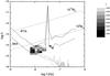 |
Fig. 6 Strain amplitude h as a function of the frequency for the BPS simulations of individual resolvable MBHBs. The gray scale gives the density distribution of the resolvable systems. Other lines are cited by the sensitivity studies (Sesana et al. 2008; Yardley et al. 2010) using the PTA detector. |
Using a 20 year-integration time, we plot in Fig. 6 the GW radiation distribution from the resolved MBHB systems in our simulation. This shows that the predicted GW radiation is below the PTA sensitivity curve. Therefore the individual SMBH sources cannot radiate sufficient GW signals for the current detector. However, these signals will be detected by SKA, the detectable number of SMBHs is about 100, which is above the SKA detection threshold. Our prediction agrees well with that of Sesana et al. (2008, 2009), and Yardley et al. (2010) (see the discussion).
Iwasawa et al. (2010) have systematically investigated the importance of eccentricity in SMBH binaries due to GW radiation. For the 100 detectable sources in Fig. 6, we also give the percentages of these sources for different eccentricities using Table 1. From it we find that the low-eccentricity binaries cannot dominate the detectable sources. The table also implies that once the individual SMBH binaries become highly eccentric, the GW radiation should be observable by the SKA detector. Meanwhile, we find for these detectable sources that the average of chirp mass ⟨ ℳchirp ⟩ = ⟨ (m1m2)3/5(m1 + m2)−1/5 ⟩ is about 8.9 × 10¹⁰ M⊙.
The percentage of detectable sources with different eccentricities (e). Note that the total number of detectable SMBH binaries in our model is 100.
4. Discussion
We have shown that there are good reasons to expect GW radiation from SMBHs and that some amplitudes will be measured by SKA in the range of 10-14 < h < 10-15. The results from a BPS approach using Monte Carlo simulations are innovative in GW radiation studies, which also regulate the calculation together with the analytical fitting functions of observation results from SDSS. In these close galaxy samples, very close SMBH binaries may produce very strong GW signals in orbital motion processes, which may be reflected by the profiles of GW forms. Especially the SMMB binaries with short orbital periods (<10 yr) may even be detectable by photometric and high-energy radiation analysis using ground-based or space telescopes. Note that the precession of orbital period caused by GW radiation from highly eccentric SMBH binaries can influence the evolution of galaxy pairs.
To study the SMBH systems such as GW sources, we needed some basic parameters for the SMBH systems (the primary BH mass m2, the secondary BH mass m1, the orbital period Porb, and so on), which were derived from the distributions of SDSS data (Ellison et al. 2008, 2010) using the polynomial curve fitting approximation. First, few studies focus on the GW radiation from SMBH systems together with the latest findings of observations, although our estimation methods are straightforward. Second, indeed, enough close galaxy pairs have been released from the SDSS data, but the error (or gray) bars (see Fig. 1 of Tamura et al. 2006; and Fig. 5 of Ellison et al. 2008) caused by the observations still exist in our simulation. Therefore a maximum ratio with respect to observations is approximately 10, which is derived from the maximum difference obtained from error bars. Third, for the redshift evolution of SMBH systems, we investigated the redshift distribution up to z ~ 0.1, which compares very well with a sky-averaged constraint on the merger rate of nearby SMBH sytems using a PTA measurement, implied by the low-redshift distance approximation r = cz/H0.
The main purpose of this study is to find out how many resolved SMBH sources we can explore with a pulsar timing detector from the GW radiation. Given the shape of the sky- and polarization-averaged sensitivity curve of the PTA (Yardley et al. 2010), the sensitivity curve is useful for comparing the strain amplitude of the GWs from an SMBH system with the average noise to see whether the individual sources can be detected by the PTA or SKA detector. A resolved source with frequency f and strain amplitude h that is observed over a time Tobs (=20 years) will appear in the Fourier spectrum of the data as a single spectral line. Therefore the SMBH systems, which are the only ones in their corresponding periodogram ranges (Δf = 1/Tobs = 1.6 × 10⁻⁹) and have higher strains than the sensitivity noise curve of the detector, are called resolved sources.
As we displayed in Fig. 6, the significantly different results can be explained as follows. Firstly, there are individual resolved SMBH systems in our nearby galaxy pairs above the predicted stochastic GW background, which is likely to be detected using the PTA in the near future (Sesana et al. 2008). Note that our estimation of GW radiation agrees with that of Sesana et al. (2008), although these authors used different methods for the underlying SMBH population, for instance, we used a precession of orbital period evolution of OJ287 and a series of derived observation results from SDSS in our simulation. Secondly, the distance was obtained using D = cz/H0, which is an acceptable approximation for relatively low redshift of galaxy pairs (Davis & Lineweaver 2004). All resolved sources in Fig. 6 are located at fairly low redshift (z < 0.1), and not at 0.2 < z < 1.5, which is one condition of Sesana et al. (2009), who predicted that their individual SMBH is below the current sensitivity. Accordingly, the major difference in the estimating the resolved sources between our model and the model of Sesana et al. (2009) arises from the distance D. Thirdly, Iwasawa et al. (2011) has pointed out that the eccentricity of most of SMBH binaries can result in a rapid merger through GW radiation. The 75% detectable sources in Fig. 6 show high eccentricities, but Yarledy et al. (2010) did not consider the eccentric SMBH binaries. Consequently, the influence of the distance and eccentricity are the main difference from other papers.
If the orbital motion of the SMBH system is appropriately reproduced using PN2 methods, we expect that the maximum GW radiation should be associated with the precise evolution trace of each BH component movement in the full relativity field. This is because the secondary BH crashes the periastron, which leads to the outburst GW signal. Furthermore, based on our estimate of the merger rate of close galaxies and making several evolutionary hypotheses, we can compute the number of SMBH sources that can be detected by the PTA (or SKA) detector. Additionally, the strength of GW signal from the merger of SMBH binaries will be blurred by other fierce energy release processes (such as supernova explosion, Mazzali et al. 2008). Finally, the evolutionary properties of SMBHs could indeed be more complex than we have described. For example, the mass transfer process between the components could be important and may even account for quasars. Meanwhile, the merging process may occur more rapidly than the evolution of SMBH, and even more BHs may reside in the core of galaxy.
To summarize, a numerical simulation of the GW radiation from the nearby galaxy pairs has been carried out using OJ287’s modulation. We used the result of SDSS data and several notable conclusions from the literature to follow the SMBH evolution using a BPS approach. In addition to a GW detector (such as SKA), we used these methods to examine the GW variation with time and estimated the number of detectable SMBH sources using observations made over 20 years. This study demonstrates the significant contribution to the GW radiation from the individual SMBH sources.
Acknowledgments
We gratefully acknowledge the BPS (Zhanwen Han and Fenghui Zhang) group at Yunnan Observatory for a discussion. We especially thank the referee for useful comments and improving of the manuscript. This work is supported by the program of the light in China’s Western Region (LCWR) (No. XBBS201022), Natural Science Foundation (No. 11103054) and Xinjiang Natural Science Foundation (No. 2011211A104). This project/publication was made possible through the support of a grant from the John Templeton Foundation. The opinions expressed in this publication are those of the authors and do not necessarily reflect the view of the John Templeton Foundation. The funds from John Templeton Foundation were awarded in a grant to The University of Chicago, which also managed the program together National Astronomical Observatories, Chinese Academy of Sciences (No. 100020101).
References
- Antonacopoulos, G. 1979, Ap&SS, 62, 217 [NASA ADS] [CrossRef] [Google Scholar]
- Begelman, M. C., Blandford, R. D., & Rees, M. J. 1980, Nature, 287, 307 [NASA ADS] [CrossRef] [Google Scholar]
- Bell, E. F., Wolf, C., Meisenheimer, K., et al. 2004, ApJ, 608, 752 [NASA ADS] [CrossRef] [Google Scholar]
- Capozziello, S., de Laurentis, M., de Paolis, F., Ingrosso, G., & Nucita, A. 2008, Mod. Phys. Lett., 23, 99 [NASA ADS] [CrossRef] [Google Scholar]
- Davis, T. M., & Lineweaver, C. H. 2004, Publ. Astron. Soc. Aust., 21, 97 [NASA ADS] [CrossRef] [Google Scholar]
- Detweiler, S. 1979, ApJ, 234, 1100 [NASA ADS] [CrossRef] [Google Scholar]
- Einstein, A. 1916, Preuss. Akad. Wiss. Berlin, Sitzungsberichte der physikalisch-mathematischen Klasse (Berlin: Springer), 688 [Google Scholar]
- Einstein, A. 1918, Preuss. Akad. Wiss. Berlin, Sitzungsberichte der physikalisch-mathematischen Klasse (Berlin: Springer), 154 [Google Scholar]
- Ellison, S. L., Patton, D. R., Simard, L., & McConnachie, A. W. 2008, AJ, 135, 1877 [NASA ADS] [CrossRef] [Google Scholar]
- Ellison, S. L., Patton, D. R., Simard, L., et al. 2010, MNRAS, 407, 1514 [NASA ADS] [CrossRef] [Google Scholar]
- Han, Z., Podsiadlowski, Ph., & Lynas-Gray, A. E. 2007, MNRAS, 380, 1098 [NASA ADS] [CrossRef] [Google Scholar]
- Hellings, R. W., & Downs, G. S. 1983, ApJ, 265, 39 [Google Scholar]
- Hobbs, G. B., Bailes, M., Bhat, N. D. R., et al. 2009, PASA, 26, 103 [NASA ADS] [CrossRef] [Google Scholar]
- Liu, J. 2009, MNRAS, 400, 1850 [NASA ADS] [CrossRef] [Google Scholar]
- Liu, J., Han, Z., Zhang, F., & Zhang, Y. 2010, ApJ, 719, 1546 [NASA ADS] [CrossRef] [Google Scholar]
- Iwasawa, M., An, S., Matsubayashi, T., Funato, Y., & Makino, J. 2011, ApJ, 731, L9 [NASA ADS] [CrossRef] [Google Scholar]
- Jaffe, A. H., & Backer, D. C. 2003, ApJ, 583, 616 [NASA ADS] [CrossRef] [Google Scholar]
- Jenet, F. A., Creighton, T., & Lommen, A. 2005, ApJ, 627, 125 [NASA ADS] [CrossRef] [Google Scholar]
- Jenet, F. A., Hobbs, G. B., van Straten, W., et al. 2006, ApJ, 653, 1571 [NASA ADS] [CrossRef] [Google Scholar]
- Kaspi, V. M., Taylor, J. H., & Ryba, M. F. 1994, ApJ, 428, 713 [NASA ADS] [CrossRef] [Google Scholar]
- Magorrian, J., Tremaine, S., Richstone, D., et al. 1998, AJ, 115, 2285 [NASA ADS] [CrossRef] [Google Scholar]
- Mazzali, P. A., Valenti, S., Della Valle, M., et al. 2008, Science, 321, 1185 [NASA ADS] [CrossRef] [PubMed] [Google Scholar]
- Menou, K., Haiman, Z., & Narayanan, V. K. 2001, ApJ, 558, 535 [NASA ADS] [CrossRef] [Google Scholar]
- Miyamoto, M., & Nagai, R. 1975, PASJ, 27, 533 [NASA ADS] [Google Scholar]
- Nelemans, G., Yungelson, L. R., & Portegies-Zwart, S. F. 2001, A&A, 375, 890 [NASA ADS] [CrossRef] [EDP Sciences] [Google Scholar]
- Paczynski, B. 1990, ApJ, 348, 485 [NASA ADS] [CrossRef] [Google Scholar]
- Rajagopal, M., & Romani, R. 1995, ApJ, 446, 543 [NASA ADS] [CrossRef] [Google Scholar]
- Ruiter, A. J., Belczynski, K., Benacquista, M., Larson, S. L., & Williams, G. B. 2010, ApJ, 717, 1006 [NASA ADS] [CrossRef] [Google Scholar]
- Sesana, A., Vecchio, A., & Colacino, C. N. 2008, MNRAS, 309, 192 [NASA ADS] [CrossRef] [Google Scholar]
- Sesana, A., Vecchio, A., & Volonteri, M. 2009, MNRAS, 394, 2255 [NASA ADS] [CrossRef] [Google Scholar]
- Sillanpaa, A., Haarala, S., Valtonen, M. J., Sundelius, B., & Byrd, G. G. 1988, ApJ, 325, 628 [NASA ADS] [CrossRef] [Google Scholar]
- Sillanpaa, A., Takalo, L. O., Pursimo, T., et al. 1996, A&A, 305, 17 [NASA ADS] [Google Scholar]
- Tamura, N., Ohta, K., & Ueda, Y. 2006, MNRAS, 365, 134 [NASA ADS] [CrossRef] [Google Scholar]
- Thorne, K. S., & Braginskii, V. B. 1976, ApJ, 204, L1 [NASA ADS] [CrossRef] [Google Scholar]
- Tremaine, S., Gebhardt, K., Bender, R., et al. 2002, ApJ, 574, 740 [NASA ADS] [CrossRef] [Google Scholar]
- Valtonen, M. J. 2007, ApJ, 659, 1074 [NASA ADS] [CrossRef] [Google Scholar]
- Valtonen, M. J., Kidger, M., Lehto, H., & Poyner, G. 2008, A&A, 477, 407 [NASA ADS] [CrossRef] [EDP Sciences] [Google Scholar]
- Wyithe, J. S. B., & Loeb, A. 2003, ApJ, 590, 691 [NASA ADS] [CrossRef] [Google Scholar]
- Yardley, D. R. B., Hobbs, G. B., Jenet, F. A., et al. 2010, MNRAS, 407, 669 [NASA ADS] [CrossRef] [Google Scholar]
- Zhang, F., Han, Z., Li, L., Shan, H., & Zhang, Y. 2010, MNRAS, 408, 1283 [NASA ADS] [CrossRef] [Google Scholar]
All Tables
The percentage of detectable sources with different eccentricities (e). Note that the total number of detectable SMBH binaries in our model is 100.
All Figures
|
Fig. 1 Orbital trace template of SMBH systems using OJ287. The primary BH is at coordinates (0, 0). The precessional elliptical curve represents the evolutionary trace of the secondary BH. |
| In the text | |
|
Fig. 2 Amplitude h as a function of the observation time for the OJ287’s model. The symbol “ ⋆ ” indicates the position at which the GW radiation from OJ287 is, ~5 × 10-16 in 2012. |
| In the text | |
|
Fig. 3 Fitting physical property curves of Monte Carlo parameters are derived from SDSS (Ellison et al. 2010) in panels a)–g), whose error bars represent the uncertainties of estimation due to the fitting errors in galaxy pairs of SDSS. The BH mass function curve is also display in panel h), which is the same as that of Tamura et al. (2006). |
| In the text | |
|
Fig. 4 Strain amplitude of GW radiation variation with time. The symbol “A” represents the average value position of the summed GW strain in each bin. The dotted line (log h = −15) marks the highest sensitivity of SKA. |
| In the text | |
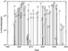 |
Fig. 5 Similar to Fig. 4, but for the luminosity variation of GW radiations with time. |
| In the text | |
|
Fig. 6 Strain amplitude h as a function of the frequency for the BPS simulations of individual resolvable MBHBs. The gray scale gives the density distribution of the resolvable systems. Other lines are cited by the sensitivity studies (Sesana et al. 2008; Yardley et al. 2010) using the PTA detector. |
| In the text | |
Current usage metrics show cumulative count of Article Views (full-text article views including HTML views, PDF and ePub downloads, according to the available data) and Abstracts Views on Vision4Press platform.
Data correspond to usage on the plateform after 2015. The current usage metrics is available 48-96 hours after online publication and is updated daily on week days.
Initial download of the metrics may take a while.