| Issue |
A&A
Volume 539, March 2012
|
|
|---|---|---|
| Article Number | A67 | |
| Number of page(s) | 11 | |
| Section | Extragalactic astronomy | |
| DOI | https://doi.org/10.1051/0004-6361/201118282 | |
| Published online | 27 February 2012 | |
Dust and gas power spectrum in M 33 (HERM33ES)⋆
1 Observatoire de Paris, LERMA & CNRS: UMR8112, 61 Av. de l’Observatoire, 75014 Paris, France
e-mail: This email address is being protected from spambots. You need JavaScript enabled to view it.
2 Laboratoire d’Astrophysique de Marseille – LAM, Université d’Aix-Marseille & CNRS, UMR7326, 38 rue F. Joliot-Curie, 13388 Marseille Cedex 13, France
3 Instituto Radioastronomia Milimetrica, Av. Divina Pastora 7, Nucleo Central, 18012 Granada, Spain
4 Institute of Astronomy and Astrophysics, National Observatory of Athens, P. Penteli, 15236 Athens, Greece
5 Argelander Institut für Astronomie, Auf dem Hügel 71, 53121 Bonn, Germany
6 Laboratoire d’Astrophysique de Bordeaux, Université Bordeaux 1, Observatoire de Bordeaux, OASU, UMR 5804, CNRS/INSU, BP 89, 33270 Floirac, France
7 University of Massachusetts, Department of Astronomy, LGRT-B 619E, Amherst, MA 01003, USA
8 IRAM-Institut de Radio Astronomie Millimétrique, 300 rue de la Piscine, 38406 Saint-Martin d’Hères, France
9 Leiden Observatory, Leiden University, PO Box 9513, 2300 RA Leiden, The Netherlands
10 ATNF, CSIRO, PO Box 76, Epping, NSW 1710, Australia
11 IPAC, MS 100-22 California Institute of Technology, Pasadena, CA 91125, USA
12 Dept. Física Teórica y del Cosmos, Universidad de Granada, Spain
13 KOSMA, I. Physikalisches Institut, Universität zu Köln, Zülpicher Straße 77, 50937 Köln, Germany
14 Department of Astronomy, Cornell University, Ithaca, NY 14853, USA
15 Max Planck Institut für Astronomie, Königstuhl 17, 69117 Heidelberg, Germany
16 JAC, 660 North A’ohoku Place, University Park, Hilo, HI 96720, USA
17 SRON Netherlands Institute for Space Research, Landleven 12, 9747 AD Groningen, The Netherlands
Received: 16 October 2011
Accepted: 17 January 2012
Abstract
Power spectra of deprojected images of late-type galaxies in gas or dust emission are very useful diagnostics of the dynamics and stability of their interstellar medium. Previous studies have shown that the power spectra can be approximated as two power laws, a shallow one on large scales (larger than 500 pc) and a steeper one on small scales, with the break between the two corresponding to the line-of-sight thickness of the galaxy disk. The break separates the 3D behavior of the interstellar medium on small scales, controlled by star formation and feedback, from the 2D behavior on large scales, driven by density waves in the disk. The break between these two regimes depends on the thickness of the plane, which is determined by the natural self-gravitating scale of the interstellar medium. We present a thorough analysis of the power spectra of the dust and gas emission at several wavelengths in the nearby galaxy M 33. In particular, we use the recently obtained images at five wavelengths by PACS and SPIRE onboard Herschel. The wide dynamical range (2–3 dex in scale) of most images allows us to clearly determine the change in slopes from −1.5 to −4, with some variations with wavelength. The break scale increases with wavelength from 100 pc at 24 and 100 μm to 350 pc at 500 μm, suggesting that the cool dust lies in a thicker disk than the warm dust, perhaps because of star formation that is more confined to the plane. The slope on small scales tends to be steeper at longer wavelength, meaning that the warmer dust is more concentrated in clumps. Numerical simulations of an isolated late-type galaxy, rich in gas and with no bulge, such as M 33, are carried out to better interpret these observed results. Varying the star formation and feedback parameters, it is possible to obtain a range of power spectra, with two power-law slopes and breaks, that nicelybracket the data. The small-scale power-law does indeed reflect the 3D behavior of the gas layer, steepening strongly while the feedback smoothes the structures by increasing the gas turbulence. M 33 appears to correspond to a fiducial model with an SFR of ~ 0.7 M⊙/yr, with 10% supernovae energy coupled to the gas kinematics.
Key words: galaxies: structure / galaxies: spiral / galaxies: ISM / Local Group / galaxies: general / galaxies: individual: M 33
Herschel is an ESA space observatory with science instruments provided by European-led Principal Investigator consortia and with important participation from NASA.
© ESO, 2012
1. Introduction
Quantifying the multi-scale structure of the interstellar medium (ISM) in galaxies is a difficult enterprise, but is rewarding since it betrays the underlying physical phenomena that control its dynamics. It has been known for a long time that the ISM reveals no preferential scale and is well represented by a fractal structure, or a power-law power spectrum. To study the atomic ISM, Crovisier & Dickey (1983) and Green (1993) studied the power spectrum as a function of the inverse scale of the 21 cm emission, and found a power law of slope between −2 and −3, independent of the distance and the velocity of the HI. This power-law slope was observed to be steeper from −3 to −4, when the broadest velocity components were averaged, thus including the warm gas, with more turbulence (Dickey et al.2001). Goldman (2000) and Stanimirovic et al.(2000) extended the ISM studies in the Milky Way to the Small Magellanic Cloud (SMC), where a power law with slopes −3.1 to −3.4 was found for the dust and gas and interpreted as 3D turbulence, although the index is shallower than the − 3.7 Kolmogorov spectrum (Stanimirovic & Lazarian 2001).
A break in scale has been searched for in order to identify the energy injection mechanism, but none has been found on small scales (i.e. smaller than 500 pc). Instead a flattening toward larger scales has been measured by Elmegreen et al.(2001) in the atomic gas of the Large Magellanic Cloud (LMC). They interpret this flattening as a change in dimensionality from 3D on small scales to 2D on large scales, where the dynamics of the galaxy plane dominates, and identify the scale of the break as the thickness of the plane. This method of finding the scale height of disks has been developed by Padoan et al.(2001), who found ~180 pc in the LMC. Recently, Block et al.(2010) have analyzed the dust maps of the LMC from Spitzer, and also confirm this break scale at 100−200 pc. From high-resolution numerical simulations fit to a late-type galaxy like the LMC, Bournaud et al.(2010) were able to retrieve the characteristics of the observed dust power spectrum. The source of turbulence could then be due to large-scale differential rotation, cold gas accretion or galaxy interactions (Lazarian et al.2001; Elmegreen & Scalo 2004). From a 2D wavelet analysis of HI in our own Galaxy, Khalil et al.(2006) find a power-law slope of −3 everywhere over the second quadrant, and do not detect the variations with velocity slices predicted by Lazarian & Pogosyan (2004). However they discover an anisotropy linked to spiral arms. The fractal approach has been widely developed for molecular clouds, which are more self-gravitating than the HI gas (Falgarone et al.1991; Pfenniger & Combes 1994; Stutzki et al.1998).
Up to now, the break scale in the HI distribution has not been identified unambiguously in external galaxies other than the LMC, although it has been searched for. Dutta et al.(2008) studied the face-on galaxy NGC 628, and find an HI power spectrum with a single power-law slope of −1.6, on the scales 0.8 to 8 kpc, since their spatial resolution is insufficient to reach the scale height of the gaseous plane. In DDO210, Begum et al.(2006) find a power-law slope of −2.75 on the scales 80 to 500 pc. This steep slope is compatible with what is found in the MW and LMC/SMC on small scales, which are driven by 3D-turbulence.
In other dwarfs also (Dutta et al.2009b), a single slope is found. The face-on galaxy NGC1058 is the first one for which the transition from 3D to 2D turbulence has been claimed (Dutta et al.2009a): the slope changes from −2.5 on 0.6 to 1.5 kpc, to −1 on 1.5−10 kpc scales. The scale height is then estimated at 490 pc, which is a relatively high value for the HI layer. In the SMC, while a steep power law is found consistently by several studies, no break scale has been found, and no transition to the 2D-turbulence (Roychowdhury et al.2010). It has been suggested that dwarf galaxies have considerably thicker gas disks than normal spiral galaxies, which supports previous studies of the thickness of dust lanes in edge-on galaxies (e.g. Dalcanton et al.2004). The transition between thick and thin gas disks was found at a mass corresponding to a circular velocity of 120 kms-1. For galaxies with low inclination on the sky plane, the thickness of gas disks can be estimated through the ratio of gas velocity dispersion to rotation (Dalcanton & Stilp 2010). The case of M 33 is exactly intermediate, with a rotational velocity of 120 kms-1. Both thick and thin disks could be expected.
Another tool for exploring the scale height of disks with higher spatial resolution, apart from studying edge-on galaxies (e.g. Bianchi & Xilouris 2011), is to study young components related to the gas, as young stars just formed out of the ISM. Elmegreen et al.(2003a) studied the power spectrum of star formation maps in nearby galaxies, and found the same behavior as for the LMC in HI: a steep power law on small scales, which is typical of 3D-turbulence, with a flattening on large scales, and a break corresponding to several hundred parsecs, typical of the plane thickness. This is true for flocculent and density-wave galaxies, although the spiral arm wave dominates at very large scales. In M 33, Elmegreen et al.(2003b) analyzed optical and Hα images and found a very shallow power law of slope −0.7, which they attribute to flattening due to contamination by strong point sources (foreground stars). For the face-on galaxy NGC 628, a shallow slope of −1.5 is found, with no break in spite of the very high spatial resolution obtained with HST (scale below 10 pc, Elmegreen et al.2006). Odekon (2008), however, finds a transition scale of about 300 pc between a steep spectrum on small scales and flattening on large scales, in the stellar distribution of M 33. This scale does not change much with the age of the stellar population considered, although the slope is steeper for the bluest and youngest stars. Sanchez et al.(2010) investigate all the young components in M 33, including young stars, HII regions and molecular clouds, and also find a clear transition region, but in the range 0.5−1 kpc. That different results are obtained for the same galaxies calls for new studies to clarify the situation.
The galaxy M 33 has been observed with Herschel PACS and SPIRE at all wavelengths by the Key Project HERM33ES, and the photometric maps are presented in Kramer et al.(2010), Boquien et al.(2010), and Verley et al.(2010). These provide high signal-to-noise maps with a wide dynamical range of scales of the dust emission at many wavelength, allowing warm and cool dust to be probed. The large and small scale structures of the gas and dust are studied through Fourier analysis. We present in Sect. 2 the different maps used, and how they are processed and deprojected to a face-on orientation. The results will be compared to numerical models, whose technique is described in Sect. 3. Results are presented for both observations and models in Sect. 4, and discussed in Sect. 5. We adopt a distance of 840 kpc for M 33 (Freedman et al.1991).
2. Observational data
To study the interstellar medium structure, we use all possible tracers, beginning by gas and dust emission (HI, CO lines, and far-infrared photometry), and also star formation from the gas (Hα, ultraviolet continuum). For the dust emission, we use Herschel observations taken in the context of the HERM33ES open time key project (Kramer et al.2010) in combination with Spitzer MIPS data (Verley et al.2007), spanning wavelengths from 24 μm to 500 μm. The Herschel PACS data covering the 100 μm and 160 μm bands have been described in Boquien et al.(2010, 2011). The SPIRE observations obtained at 250, 350, and 500 μm are displayed in Kramer et al.(2010) and Verley et al.(2010).
Characteristics of the different maps used.
We also use ground-based Hα observations presented in Hoopes et al.(2001) to trace the current (~10 Myr) star formation and GALEX data (Thilker et al.2005; Gil de Paz et al.2007) to trace the recent (~100 Myr) star formation. To trace the atomic gas, we use the HI 12′′resolution map published in Gratier et al.(2010), and for the molecular gas, their partial CO(2−1) 12′′resolution map (Gratier et al.2010). All useful characteristics of the images are summarized in Table 1. All maps have been deprojected, with the adopted inclination of 56° and position angle of 22.5°, before Fourier analysis.
The data analyzed in the present work are more appropriate than earlier data (Elmegreen et al.2003b; Odekon 2008; Sanchez et al.2010) to study the power spectra and the structure of the interstellar medium, since they refer directly to the gas and dust in M 33, and they have the dynamical range (from 40 pc to 20 kpc) and spatial resolution to reveal the thickness of the gas layer. The gas and dust emission trace directly the collisional material, with no intervening and perturbing emission (like galactic stars).
3. Numerical model
To compare with what is expected from the dynamical instabilities of the interstellar medium, we ran idealized simulations, fit for a late-type galaxy without bulge and rich in gas like M 33.
3.1. Technique
The numerical code is based on the TREE/SPH version developed by Semelin & Combes (2005) and di Matteo et al.(2007), with star formation and feedback. The TREE gravitational part of the code deals with two collisionless components: the stars and the dark matter, which differ only by their initial conditions. It also deals with the gas component, whose hydrodynamics is treated with the SPH (smooth particle hydrodynamics) algorithm, using adaptive resolution. The softening parameter or the spatial resolution of gravity is taken to be 30 pc, and the average size of a gaseous particle (the SPH kernel, or spatial resolution of the hydrodynamics) is also around 30 pc, although it can drop down to 3 pc in overdense regions. The number of particles is 1.2 million, with 0.6 million gas particles, 0.4 million dark matter particles, and 0.2 million “stars” at the beginning of the simulations. The gas particles are assumed to follow an isothermal equation of state with pressure forces corresponding to a sound velocity of 6 kms-1 in the fiducial model. Shocks are treated with a conventional form of artificial viscosity, with parameters given in di Matteo et al.(2007). All physical quantities (density and forces) are computed by averaging over a number of 50 neighbors. The equations of motion are integrated using a leapfrog algorithm with a fixed time step of 0.3 Myr.
Star formation is taken into account in most models, with an assumed Schmidt law, of exponent n = 1.5, i.e. for each gas particle of mass Mgas, and volumic density ρgas computed over its neighbors: 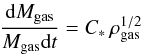 where in most runs, the star formation constant C∗ is calibrated such that the gas consumption time scale is of the order of 2 Gyr (then C∗ = C0). To check its influence on the gas scale height, C∗ is increased in some of the runs. In most simulations, the density threshold for star formation is set very low (2 × 10⁻⁶ atoms cm-3), and is then increased in a few runs (up to 4 atoms cm-3). Star formation is then taken into account for each gas particle, using the hybrid particles scheme (e.g. di Matteo et al.2007), before sufficient stellar mass is accumulated and a star particle can be created. Continuous mass loss is also considered, with about 40% of the stellar mass loss by young massive stars after 5 Gyr (Jungwiert et al.2001).
The energy reinjected by supernovae into the interstellar medium is assumed to be a kinematic feedback on neighboring gas particles: each neighbor of an SPH particle having formed δm of stars is given a radial kick in velocity away from the supernova formed. The energy available is computed from δm, assuming a Scalo IMF (about 0.5% of the stars formed have a mass higher than 8 M⊙ and explode as supernovae), the energy of a supernova ESN = 1051 erg is distributed to the 50 neighbors according to their weight (the SPH kernel), with an efficiency ϵ that has been varied from 10-4 to 1, with 10% as the fiducial value (see Table 2). For the fiducial feedback efficiency, a particle might get a kick of ~1 kms-1 at each time step, and for the extreme feedback, it can reach 5 kms-1. The efficiency of the feedback is not well known, and it depends on the coupling of the supernovae and the gas (whether the young stars have already left their birth clouds when they explode, etc.). Some energy and supernova explosions are also due to the old population of stars (e.g. Dopita 1985).
Initial conditions of the simulations.
3.2. Initial conditions
The initial stellar component of the galaxy is selected to be of type Scd, similar to the M 33 galaxy. The stellar and gaseous disks are represented initially by Miyamoto-Nagai functions, with characteristic height parameters of 170 pc and 70 pc, respectively. The stellar disk has a mass of 0.5 × 10¹⁰ M⊙ with a characteristic radius of 2 kpc, while the gas disk has a mass of 1.5 × 10⁹ M⊙ with a radius 2.5 kpc. Both are embedded in a spherical halo of dark matter, represented by a Plummer sphere of mass 4 × 10¹⁰ M⊙ within 18 kpc, with a characteristic radius of 9.5 kpc.
The initial stability of the gas and stellar disks is controlled by the Toomre parameter Q, ratio of the radial component of the velocity dispersion to the critical one σcrit = 3.36GΣ/κ, where Σ is the disk surface density of the component (gas or stars), and κ the epicyclic frequency. We select equal Toomre parameters for gaseous and stellar disks. The azimuthal velocity dispersions verify the epicyclic ratio σθ/σr = κ/2Ω initially, and the z-components are fixed by the isothermal equilibrium of the disks in the vertical direction.
The gas is isothermal, but its equivalent velocity dispersion, governing the pressure, may be varied between 6 and 12 kms-1. The recipes for star formation: efficiency, density threshold, and feedback, are also varied. They have a strong impact on the interstellar gas structure.
The initial conditions of the runs described here are given in Table 2. The rotation curve corresponding to one of the runs is plotted in comparison to the data points in Fig. 1. All runs have similar rotation curves. Given the uncertainties, all the rotation curves are compatible with the data.
 |
Fig. 1 Rotation curve for our late-type Scd model, compared to the observed points (symbols and error bars) compiled for M 33 by Corbelli & Salucci (2007). In addition to the circular velocity of the model, the characteristic frequencies Ω, Ω − κ/2, etc. are plotted. |
 |
Fig. 2 2D power spectrum for the PACS 100 μm image. The color scale is in arbitrary units. |
 |
Fig. 3 Power spectrum of the Spitzer-MIPS 70 μm map and the PACS-100 μm dust emission map of M 33. The vertical dashed line to the right represents the spatial resolution of the observations on the major axis. Since the deprojection to a face-on galaxy implies a factor 1 ! cos(56°) = 1.79 larger beam on the minor axis, we have also plotted a second dashed vertical line to the left, indicating the geometric mean of the resolution on both minor and major axes. Statistical error bars are given in this first figure, and then omitted later for clarity. They are significant only at the largest scales (small k), where the statistical errors are the largest. The red lines are power-law fits, minimizing the χ2, as explained in the text. |
4. Results
4.1. Power spectrum of the data
The power spectra of the 2D projected maps were analyzed through the 2D Fourier transform:  where F(x,y) is the intensity of each pixel, and kx and ky are the wave number, conjugate to x and y, varying as the inverse of scale. The full 2D power spectrum is given by
 ![Mathematical equation: \begin{equation*} P\left(k_x, k_y\right) = \left({\rm Re} {\left[F^*\right]}\right)^2 + \left({\rm Im} {\left[F^*\right]}\right)^2. \end{equation*}](/articles/aa/full_html/2012/03/aa18282-11/aa18282-11-eq63.png) An example of a 2D power spectrum is given for the PACS-100 μm image in Fig. 2. The 1D power spectrum P(k) can be calculated through azimuthal averaging, in the (kx,ky) plane, using
An example of a 2D power spectrum is given for the PACS-100 μm image in Fig. 2. The 1D power spectrum P(k) can be calculated through azimuthal averaging, in the (kx,ky) plane, using  . The power spectra P(k) are plotted for the various maps in Figs. 3–8. Two slopes have been fit at small (ss) and large scales (LS), and the different values can be found in Table 3, together with the break scale separating the two regimes. In most of the cases, the power spectra clearly show two different regimes with different slopes, and small and large-scales, for scales larger than the spatial resolution. A knee is apparent between the two regimes (ss and LS), and indicates the break scale. We used a least-square-fit program to determine the slopes of the two power laws, and left open the position of the separation between the two straight lines. Varying the value of the separation, we selected for the break the value that minimizes the sum of the χ2 of the two line fits (ss and LS). In general the minimum is quite clear. There is one ambiguous case, however, that is the HI map in Fig. 8. The two slopes are close and the determination less trustworthy. Examples of the deprojected images of the Herschel dust emission are displayed in Figs. 9 and 10. In addition to the power spectra, the azimuthal large-scale structure develops spiral arms, which are quantified and studied in Appendix A. Determining the break scale is obviously more secure when it is found significantly to be larger than the resolution scale of the observations. We tested the effect of spatial resolution by smoothing the PACS-100 μm map in Appendix B. In the observed power spectra (e.g. Figs. 3–7), the limit of the instrumental resolution is clearly seen, through the sudden change from a straight line to a dropping curve, at large k. We have indicated the value of the resolution scale on the major axis and also the geometric mean of the resolution on both minor and major axis, since the deprojection to a face-on galaxy implies a factor 1/cos(56°) = 1.79 larger beam on the minor axis. We conclude from Appendix B that those break scales that are at least twice larger than the beam scale are robust with respect to the resolution effect.
Power-law slopes and breaks for observations.
 |
Fig. 9 Deprojected maps of the dust at 100 (left) and 160 μm (right). The major axis has been rotated to be vertical. The color scale is in arbitrary units. |
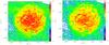 |
Fig. 10 Deprojected maps of the dust at 250 (left) and 500 μm (right). The major axis has been rotated to be vertical. The color scale is in arbitrary units. |
We also tested the robustness of our determinations by computing the power spectra using only one side of the galaxy. The easiest way to compute that, with the same algorithm, was to remove in the map one half of the galaxy, say the southern part, and complete the map by extending the northern part by point symmetry through the center. For all maps, the different slopes and break scales for the two sides of the galaxy are also displayed in Table 3, where the last columns display the extreme values found for the slopes and breaks. This procedure maximizes the error bars, especially in the LS slopes, since the norhern part of M 33 is quite different from the southern part. The slopes are determined with an error bar of the order of ± 0.2 in general, and the break scales are even more robust, within 15%. We also checked the effect of smoothing on the maps. As expected, the power spectrum on large-scales is unchanged, and only the power at the extreme of the small-scales of the spatial resolution drops. The break scale is also enlarged by the resolution, when it is too close, and we can see for instance that the break at 70 μm is larger than at 24 and 100 μm (Table 3) only because of the coarser resolution. That some maps have a smaller pixel size than the Nyquist size (half of the nominal resolution) does not influence the results. We have truncated the power spectra at the Nyquist sampling in the figures.
In Tables 1 and 3 it is ovious that the break scale is affected by the spatial resolution of the maps. Five maps have a ratio between break and resolution scales lower or equal to 3 (NUV, the 3 SPIRE, and CO), for the others, the ratio is 3.8 (FUV), 12.5 (Hα), 4.2 (MIPS-24 μm), 3.9 (MIPS-70 μm), 3.9 (PACS-100 μm), 3.6 (PACS-160 μm) and 3.3 (HI). For those, the determination of the break appears significant. As for the slope determination, the large-scale ones are not affected, and their variation is meaningful: the LS-slopes are flatter for the star-formation tracers than for the dust and gas, and they are growing steeper with wavelength.
It is interesting to note that the Hα map, which traces gas ionized by the UV photons from massive stars and, indirectly, current star formation, has power-spectrum slopes significantly flatter than the other power spectra of the ISM components. This might be expected, since star formation gives more power to the small scales. Its break scale, related to the plane thickness is higher. The GALEX FUV and NUV, which trace the recent, but past, star formation, have slopes that are more comparable to the other ISM slopes however, and have smaller break scales, implying thinner layers. The break scale in Hα is larger than in the UV because Hα traces the ionized gas, and only indirectly the young stars. The ionized layer may be thicker, affected by bubbles, filaments, and fountain effects associated to star formation.
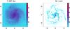 |
Fig. 11 Face-on projection of the run 2 model, at T = 667 Myr. Left are the stars, and right, the gas. The linear scales on both axes are in kpc, and the color scale is in arbitrary units. |
 |
Fig. 12 Face-on projection of the run 3 model, at T = 667 Myr. Left are the stars, and right, the gas. The linear scales on both axes are in kpc, and the color scale is in arbitrary units. |
 |
Fig. 13 Face-on projection of the run 4 model, at T = 667 Myr. Left are the stars, and right, the gas. |
 |
Fig. 14 Face-on projection of the run 7 model, at T = 667 Myr. Left are the stars, and right, the gas. |
 |
Fig. 15 Face-on projection of the run 8 model, at T = 667 Myr. Left are the stars, and right, the gas. |
 |
Fig. 16 Face-on projection of the run 9 model, at T = 667 Myr. Left are the stars, and right, the gas. |
 |
Fig. 17 Power spectrum of the gas in model runs 1 and 2. The vertical dashed line represents the softening length of the gravity. |
 |
Fig. 18 Power spectrum of the gas in model runs 3 and 4. |
 |
Fig. 19 Power spectrum of the gas in model runs 7 and 8. |
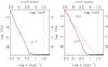 |
Fig. 20 Power spectrum of the stellar component in runs 2 and 7. The vertical dashed line represents the softening length of the gravity. |
Power-law slopes and breaks for simulations.
The dust emissions at various wavelengths have quite compatible power spectra. Their different break scales reflect the increasing beam size with wavelength. The molecular component appears thinner than the atomic one, although spatial resolution might influence its break scale.
Independent of the spatial resolutions, the slope of the power spectra on small scales are steeper at large wavelengths for the dust emission. Between 250 and 500 μm, the SPIRE maps have slopes between −4.3 and −4.7, while the MIPS and PACS maps between 24 and 100 μm have slopes ranging between −2.7 and −3.8. This is significant, and tends to show that the cool dust has less small-scale structure, since individual cloud cores are invisible.
4.2. Power spectrum of the model
The various runs develop different gas structure and clumpiness, as can be seen in Figs. 11 to 16, owing to different factors: first initial conditions that are selected to be more or less stable, second different sub-grid “temperatures” of the gas, and finally the star formation rate and feedback. Some galaxies, which are launched with initial conditions among the stablest, can end up with a more perturbed morphology and stronger turbulence than others that began more unstable, due to more supernovae feedback.
We computed the Fourier analysis in the same way on the gas maps obtained in the numerical simulations. The derived results are converging toward the same values at the middle of the runs, and we plot all of them for the final snapshots at T = 667 Myr for the sake of simplicity (cf. Figs. 17–19). For comparison, we also plot the power spectrum of some old stellar components, which have almost only one power law (Fig. 20). These correspond to runs 2 and 7 at T = 667 Myr. There is structure until about 300 pc, and no small-scale component, as expected for a collisionless component.
The first result that is obvious in Table 4 is that the predictions of the models bracket the values obtained in the observations, both in the slopes on large and small scales and in the break scales. Those can be compared to the actual thickness of the gas layer in the simulations. This is done in Table 4, showing that the break scale does not follow the thickness closely. Although both should be similar when only the self-gravity of the gas is taken into account, their close relation is blurred by other factors and in particular the feedback efficiency. When the feedback is too extreme, the small scale structure of the gas is smoothed out, even toward a larger scale than the vertical thickness. Therefore the range of break scales is wider than the range of possible plane heights.
The main parameters that control the turbulence, hence the power spectrum of the gas structure, are the star formation rate, the amount of feedback, but also the assumed equivalent temperature of the gas or sound speed, which is directly involved in the pressure forces. Increasing the turbulence by supernovae feedback efficiently suppresses the small-scale structure (power-law slopes of ~−5.) and thickens the gas layer and the corresponding break scale substantially. Without star formation and feedback, it is only possible to have gas morphologies comparable to the observed ones if a minimum sound speed of 12 kms-1 is injected. Figures 11 to 16 show the wide variety of gas structures, according to the variations in those parameters. It appears that our fiducial model (run4) is the one that corresponds the best to the M 33 galaxy, both for its morphology and for the typical power-law slopes and break scale. It has a star formation rate of ~0.7 M⊙/yr, and a feedback such that 10% of supernovae energy is coupled to the kinematics of the gas. Verley et al.(2009) found a star formation rate of 0.5 M⊙/yr for M 33.
5. Discussion and conclusions
We have presented the Fourier analysis of dust and gas emission maps of M 33 at several wavelengths and compared them with the Hα and UV maps, which trace recent star formation. We find that all the power spectra can be decomposed into two regimes, a large-scale (>500 pc) power law, of −1.5 < slopeLS < −1.0, and a steeper small-scale one, with −4.0 < slopess < −3.0. The latter slopes correspond quite well to what is found for the Milky Way (Dickey et al.2001) or the Small Magellanic Cloud (Stanimirovic et al.2000). The Hα star formation tracer has shallower power spectra, indicating more power on small scales. The break scale is in the range 100−150 pc for the dust and the gas, increasing at large wavelengths, probably influenced by the progressive lack of spatial resolution. The Hα break scale is significantly higher (300 pc), implying a thicker layer for ionized gas, while the UV layers appears thinner (65 pc). This might be understood considering that UV originates in stars that are concentrated in the disk whereas the ionized gas could be present quite far from the plane of the disk. Giant HII regions typically have round shapes and are not as confined to the disk. Tabatabaei et al.(2007) have already shown with wavelets that the Hα map is dominated by giant HII regions, which are bubble-like with sizes from 100 to 500 pc. By comparison the diffuse component is weaker, which flattens the Fourier ss-slope, and enlarges the break scale. Although the warm dust in the MIPS-24 μm map is also related to the young star formation, there are no such large bubbles, only the point sources are prominent inside the bubble, as can be seen in Fig. 3 of Verley et al.(2010). This explains the different break scales between Hα and MIPS-24 μm maps.
It is also possible that the large thickness suggested by the Hα analysis is related to the diffuse ionized gas (DIG) observed in several edge-on galaxies to follow a rather thick layer of about 1 kpc height (see a review by Dettmar 1992). This extra-planar ionized gas is thought to be due to star formation, and it is present in about 40% of 74 edge-on galaxies (Rossa & Dettmar 2003). It can be widely diffuse or take the shape of filaments, plumes, and bubbles (Rand 1997). These extraplanar extensions could be due to UV ionizing photons escaping the star-forming regions, supernovae feedback, fountain effects, chimneys, and be part of an active disk-halo interaction, with exchange of matter (Howk & Savage 2000).
The comparison with simulated models tells us that the observation of a break in the power spectrum of observed gas distribution is not always related to the 2D/3D transition, and it indicates the thickness of the gaseous disk only when the latter is not heated by a strong star formation rate and a strong supernovae feedback. For a quiescent galaxy, the break should still be an indication of the gas layer thickness.
Block et al.(2010) found in the LMC that the small scale slopes of the power spectra were steeper at longer wavelengths; i.e., the cool dust was smoother than the hot emission. We find a similar result. The slope of the SPIRE maps are around −4.5, while the warmer dust at 24−100 μm has an average slope of −3.2. This observation can be interpreted in terms of star formation occuring in the clumpy medium. Once the stars are formed, they heat the dust around, which explains why the emission at shortest wavelength (warmer dust) is clumpier. Also the break scale, hence the thickness of the plane, is larger for the cold gas. This could in addition be because the cold component is much more extended in radius (Kramer et al.2010), and it is well known that the gas layer is flaring in the outer parts of galaxies. As for the gas emission, the molecular gas appears clumpier, but only slightly more so than the atomic gas. And the break occurs on about the same scale. Since it is likely that, in the relatively quiescent M 33 galaxy, the break indicates the thickness of the gas layer, this situation is not like the Milky Way, where the CO component is significantly thinner than the HI (Bronfman et al.1988). A thick CO layer, three times as wide as the dense molecular gas layer and comparable to the HI layer, has been observed (Dame & Thaddeus 1994), but it involves a low mass. As a galaxy of intermediate mass, M 33 could indeed have a thicker gas layer than the Milky Way (Dalcanton et al.2004).
We also showed that numerical models predict gas morphologies and small-scale power laws that bracket the observational data. It is possible to obtain a colder or a more turbulent interstellar medium by varying the star formation feedback and the sound speed of the gas. The Fourier analysis of the models reveals that the break scale is a good indicator of the actual thickness of the gas layer, although it varies within a wider range when extreme feedback is used, and smoothes out the small-scale gas structures. The power-law slopes obtained in the models on large and small scales reflect the gas morphology and turbulence quite accurately. Fourier analyzes are therefore a good tool for determining the thickness of the gas plane, at any orientation on the plane of the sky, and the actual physical state of the gas, in its star formation phase. The current models are not devoid of shortcomings however, since they only partly allow distinguishing between the 12 different tracers of the gas phase observed here, such as radiative transport and dust properties are not taken into account.
Comparison of power spectrum analysis between galaxies should allow one to determine their relative star formation rate and feedback. This will however need high spatial resolution maps, such as the ones that will be provided with ALMA.
The gas plane in M 33 appears relatively thick and turbulent, with respect to our closest fiducial model, which could be a consequence of its recent heating in particular through the M31 interaction (McConnachie et al.2009).
Acknowledgments
We warmly thank the anonymous referee for his/her constructive comments and suggestions. We made use of the NASA/IPAC Extragalactic Database (NED).
References
- Begum, A., Chengalur, J. N., & Bhardwaj, S. 2006, MNRAS, 372, L33 [NASA ADS] [Google Scholar]
- Bianchi, S., & Xilouris, E. M. 2011, A&A, 531, L11 [NASA ADS] [CrossRef] [EDP Sciences] [Google Scholar]
- Block, D. L., Puerari, I., Elmegreen, B. G., & Bournaud, F. 2010, ApJ, 718, L1 [NASA ADS] [CrossRef] [Google Scholar]
- Boquien, E., Calzetti, D., Kramer, C., et al. 2010, A&A, 518, L70 [NASA ADS] [CrossRef] [EDP Sciences] [Google Scholar]
- Boquien, E., Calzetti, D., Combes, F., et al. 2011, AJ, 142, 111 [NASA ADS] [CrossRef] [Google Scholar]
- Bournaud, F., Combes, F., Jog, C. J., & Puerari, I. 2005, A&A, 438, 507 [NASA ADS] [CrossRef] [EDP Sciences] [Google Scholar]
- Bournaud, F., Elmegreen, B. G., Teyssier, R., Block, D. L., & Puerari, I. 2010, MNRAS, 409, 1088 [NASA ADS] [CrossRef] [Google Scholar]
- Braine, J., Gratier, P., Kramer, C., et al. 2010, A&A, 518, L69 [NASA ADS] [CrossRef] [EDP Sciences] [Google Scholar]
- Bronfman, L., Cohen, R. S., Alvarez, H., et al. 1988, ApJ, 324, 248 [NASA ADS] [CrossRef] [Google Scholar]
- Corbelli, E., & Salucci, P. 2007, MNRAS, 311, 441 [Google Scholar]
- Crovisier, J., & Dickey, J. 1983, A&A, 122, 282 [NASA ADS] [Google Scholar]
- Dalcanton, J. J., & Stilp, A. M. 2010, ApJ, 721, 547 [NASA ADS] [CrossRef] [Google Scholar]
- Dalcanton, J. J., Yoachim, P., & Bernstein, R. 2004, ApJ, 608, 189 [NASA ADS] [CrossRef] [Google Scholar]
- Dame, T. M., & Thaddeus, P. 1994, ApJ, 436, L173 [NASA ADS] [CrossRef] [Google Scholar]
- Dettmar, R. J. 1992, Fund. Cosm. Phys., 15, 143 [Google Scholar]
- Di Matteo, P., Combes, F., Melchior, A.-L., & Semelin, B. 2007, A&A, 468, 61 [NASA ADS] [CrossRef] [EDP Sciences] [Google Scholar]
- Dickey, J. M., McClure-Griffiths, N. M., Stanimirovic, S., Gaensler, B. M., & Green, A. J. 2001, ApJ, 561, 264 [NASA ADS] [CrossRef] [MathSciNet] [Google Scholar]
- Dopita, M. A. 1985, ApJ, 295, L5 [NASA ADS] [CrossRef] [Google Scholar]
- Dutta, P., Begum, A., Bharadwaj, S., & Chengalur, J. N. 2008, MNRAS, 384, L34 [NASA ADS] [Google Scholar]
- Dutta, P., Begum, A., Bharadwaj, S., & Chengalur, J. N. 2009a, MNRAS, 397, L60 [NASA ADS] [Google Scholar]
- Dutta, P., Begum, A., Bharadwaj, S., & Chengalur, J. N. 2009b, MNRAS, 398, 887 [NASA ADS] [CrossRef] [Google Scholar]
- Elmegreen, B. G., & Scalo, J. 2004, ARA&A, 42, 211 [NASA ADS] [CrossRef] [Google Scholar]
- Elmegreen, B.G., Kim, S., & Staveley-Smith, L. 2001, ApJ, 548, 749 [NASA ADS] [CrossRef] [Google Scholar]
- Elmegreen, B. G., Elmegreen, D. M., & Leitner, S. N. 2003a, ApJ, 590, 271 [NASA ADS] [CrossRef] [Google Scholar]
- Elmegreen, B. G., Leitner, S. N., Elmegreen, D. M., & Cuillandre, J.-C. 2003b, ApJ, 593, 333 [NASA ADS] [CrossRef] [Google Scholar]
- Elmegreen, B. G., Elmegreen, D. M., Chandar, R., Whitmore, B., & Regan, M. 2006, ApJ, 644, 879 [NASA ADS] [CrossRef] [Google Scholar]
- Falgarone, E., Phillips, T. G., & Walker, C. K. 1991, ApJ, 378, 186 [NASA ADS] [CrossRef] [Google Scholar]
- Freedman, W. L., Wilson, C. D., & Madore, B. F. 1991, ApJ, 372, 455 [NASA ADS] [CrossRef] [Google Scholar]
- Gil de Paz, A., Boissier, S., Madore, B. F., et al. 2007, ApJS, 173, 185 [NASA ADS] [CrossRef] [Google Scholar]
- Goldman, I. 2000, ApJ, 541, 701 [NASA ADS] [CrossRef] [Google Scholar]
- Gratier, P., Braine, J., Rodriguez-Fernandez, N. J., et al. 2010, A&A, 522, A3 [NASA ADS] [CrossRef] [EDP Sciences] [Google Scholar]
- Green, D. A. 1993, MNRAS, 262, 327 [NASA ADS] [CrossRef] [Google Scholar]
- Hoopes, C. G., Walterbos, R. A. M., & Bothun, G. D. 2001, ApJ, 559, 878 [NASA ADS] [CrossRef] [Google Scholar]
- Howk, J. C., & Savage, B. D. 2000, AJ, 119, 644 [NASA ADS] [CrossRef] [Google Scholar]
- Jungwiert, B., Combes, F., & Palous, J. 2001, A&A, 36, 85 [NASA ADS] [CrossRef] [EDP Sciences] [Google Scholar]
- Khalil, A., Joncas, G., Nekka, F., Kestener, P., & Arneodo, A. 2006, ApJS, 165, 512 [NASA ADS] [CrossRef] [Google Scholar]
- Kramer, C., Buchbender, C., Xilouris, E. M., et al. 2010, A&A, 518, L67 [NASA ADS] [CrossRef] [EDP Sciences] [Google Scholar]
- Lazarian, A., & Pogosyan, D. 2004, ApJ, 616, 943 [NASA ADS] [CrossRef] [Google Scholar]
- Lazarian, A., Pogosyan, D., Vázquez-Semadeni, E., & Pichardo, B. 2001, ApJ, 555, 130 [NASA ADS] [CrossRef] [Google Scholar]
- McConnachie, A. W., Irwin, M. J., Ibata, R. A., et al. 2009, Nature, 461, 66 [NASA ADS] [CrossRef] [PubMed] [Google Scholar]
- Odekon, M. C. 2008, ApJ, 681, 1248 [NASA ADS] [CrossRef] [Google Scholar]
- Padoan, P., Kim, S., Goodman, A., & Staveley-Smith, L. 2001, ApJ, 555, L33 [NASA ADS] [CrossRef] [Google Scholar]
- Pfenniger, D., & Combes, F. 1994, A&A, 285, 94 [NASA ADS] [Google Scholar]
- Rand, R. J. 1997, ApJ, 474, 129 [NASA ADS] [CrossRef] [Google Scholar]
- Rossa, J., & Dettmar, R. J. 2003, A&A, 406, 493 [NASA ADS] [CrossRef] [EDP Sciences] [Google Scholar]
- Roychowdhury, S., Chengalur, J. N., Begum, A., & Karachentsev, I. D. 2010, MNRAS, 404, L60 [NASA ADS] [CrossRef] [Google Scholar]
- Sanchez, N., Anez, N., Alfaro, E. J., & Crone Odekon, M. 2010, ApJ, 720, 541 [NASA ADS] [CrossRef] [Google Scholar]
- Semelin, B., & Combes, F. 2005, A&A, 441, 55 [NASA ADS] [CrossRef] [EDP Sciences] [Google Scholar]
- Stanimirovic, S., & Lazarian, A. 2001, ApJ, 551, L53 [NASA ADS] [CrossRef] [Google Scholar]
- Stanimirovic, S., Staveley-Smith, L., van der Hulst, J. M., et al. 2000, MNRAS, 315, 791 [NASA ADS] [CrossRef] [Google Scholar]
- Stutzki, J., Bensch, F., Heithausen, A., Ossenkopf, V., & Zielinsky, M. 1998, A&A, 336, 697 [NASA ADS] [Google Scholar]
- Tabatabaei, F. S., Beck, R., Krause, M., et al. 2007, A&A, 466, 509 [NASA ADS] [CrossRef] [EDP Sciences] [Google Scholar]
- Thilker, D. A., Hoopes, C. G., Bianchi, L., et al. 2005, ApJ, 619, L67 [NASA ADS] [CrossRef] [Google Scholar]
- Verley, S., Hunt, L. K., Corbelli, E., & Giovanardi, C. 2007, A&A, 476, 1161 [NASA ADS] [CrossRef] [EDP Sciences] [Google Scholar]
- Verley, S., Corbelli, E., Giovanardi, C., & Hunt, L. K. 2009, A&A, 493, 453 [NASA ADS] [CrossRef] [EDP Sciences] [Google Scholar]
- Verley, S., Relano, M., Kramer, C., et al. 2010, A&A, 518, L68 [NASA ADS] [CrossRef] [EDP Sciences] [Google Scholar]
Appendix A: Fourier analysis of the density
Until now, we have essentially analyzed the small scale structure of the interstellar medium in various tracers, but ignored the azimuthal dependence. The different tracers also reveal a contrasted spiral structure that is interesting to present, at least in two representative deprojected maps, the Herschel 100 μm image (dust and gas images show similar features) and the Hα image (star formation, similar to UV images).
 |
Fig. A.1 Left: radial variations of Am, for m = 1 − 4, the normalized Fourier amplitudes of the deprojected 100 μm image of M 33. Right: corresponding radial variations of the phases Φm in radians. |
We computed the Fourier transform of the corresponding surface densities, decomposed as  where the normalized strength of the Fourier component m is Am(r) = am(r)/μ0(r). Thus, A2 represents the normalized amplitude for a m = 2 distortion like a bar or spiral arm, at a given radius, and A1 represents the same for the disk lopsidedness. The quantity φm denotes the position angle or the phase of the Fourier component m. Such a density analysis was done for example by Bournaud et al.(2005), to study asymmetries and lopsidedness in galaxies, and correlate it with m = 2 features.
 |
Fig. A.2 Left: radial variations of Am, for m = 1 − 4, the normalized Fourier amplitudes of the deprojected Hα image of M 33. Right: corresponding radial variations of the phases Φm in radians. |
Figure A.1 shows a plot of the amplitude Am(r) and the phase φm(r) versus radius r for M 33, at 100 μm and Fig. A.2, the same for Hα. Both show a prominent spiral feature at radii ~ 3–4 kpc, with a phase decreasing slightly with radius, in the direct sense. The m = 2 distortions show accompanying m = 4 harmonics. The lopsidedness also increases with radius, while the corresponding phase is fairly constant.
These plots show that the spiral structure in M 33 is mildly contrasted, in both gas and SFR tracers. Indeed, the normalized m = 2 amplitude is between 0.4 and 0.8. There is also a significant asymmetry and lopsidedness, as testified by the strong m = 1 amplitude comparable with the m = 2. This explains why the slopes on large scales were more different between the two halves of the galaxy than the small-scale ones. This large asymmetry could be due to the current interaction between M 33 and M31 (McConnachie et al.2009).
Appendix B: The effect of resolution
We have explored the effect of spatial resolution in the determination of the various slopes and break scales, in smoothing the PACS-100 μm map at various resolutions, from the original 7′′to 11, 18, 26, and 36′′, corresponding to 44, 72, 104, and 144 pc on the major axis. The resulting fits are shown in Figs. B.1 and B.2, to be compared with Fig. 3. The break scales are 97, 111, 135, and 195 pc, instead of 93 pc for the original 7′′resolution. The determination is possible only for the two first cases.
 |
Fig. B.1 Power spectrum of the PACS 100 μm map, at degraded resolutions of 11 and 18′′. The vertical dashed line to the right represents the smoothed spatial resolution on the major axis. Since the deprojection to a face-on galaxy implies a factor 1 ! cos(56°) = 1.79 larger beam on the minor axis, we have also plotted a second dashed vertical line to the left, indicating the geometric mean of the resolution on both the minor and major axes. |
All Tables
All Figures
|
Fig. 1 Rotation curve for our late-type Scd model, compared to the observed points (symbols and error bars) compiled for M 33 by Corbelli & Salucci (2007). In addition to the circular velocity of the model, the characteristic frequencies Ω, Ω − κ/2, etc. are plotted. |
| In the text | |
|
Fig. 2 2D power spectrum for the PACS 100 μm image. The color scale is in arbitrary units. |
| In the text | |
|
Fig. 3 Power spectrum of the Spitzer-MIPS 70 μm map and the PACS-100 μm dust emission map of M 33. The vertical dashed line to the right represents the spatial resolution of the observations on the major axis. Since the deprojection to a face-on galaxy implies a factor 1 ! cos(56°) = 1.79 larger beam on the minor axis, we have also plotted a second dashed vertical line to the left, indicating the geometric mean of the resolution on both minor and major axes. Statistical error bars are given in this first figure, and then omitted later for clarity. They are significant only at the largest scales (small k), where the statistical errors are the largest. The red lines are power-law fits, minimizing the χ2, as explained in the text. |
| In the text | |
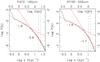 |
Fig. 4 Same as Fig. 3, for the power spectrum of the PACS-160 μm and SPIRE-250 μm dust map. |
| In the text | |
 |
Fig. 5 Same as Fig. 3, for the power spectrum of the SPIRE-350 μm and 500 μm cool dust map. |
| In the text | |
 |
Fig. 6 Same as Fig. 3, for the power spectrum of the Hα and MIPS-24 μm maps. |
| In the text | |
 |
Fig. 7 Same as Fig. 3, for the power spectrum of the GALEX NUV and FUV maps. |
| In the text | |
 |
Fig. 8 Same as Fig. 3, for the power spectrum of the HI and CO(2 − 1) maps. |
| In the text | |
|
Fig. 9 Deprojected maps of the dust at 100 (left) and 160 μm (right). The major axis has been rotated to be vertical. The color scale is in arbitrary units. |
| In the text | |
|
Fig. 10 Deprojected maps of the dust at 250 (left) and 500 μm (right). The major axis has been rotated to be vertical. The color scale is in arbitrary units. |
| In the text | |
|
Fig. 11 Face-on projection of the run 2 model, at T = 667 Myr. Left are the stars, and right, the gas. The linear scales on both axes are in kpc, and the color scale is in arbitrary units. |
| In the text | |
|
Fig. 12 Face-on projection of the run 3 model, at T = 667 Myr. Left are the stars, and right, the gas. The linear scales on both axes are in kpc, and the color scale is in arbitrary units. |
| In the text | |
|
Fig. 13 Face-on projection of the run 4 model, at T = 667 Myr. Left are the stars, and right, the gas. |
| In the text | |
|
Fig. 14 Face-on projection of the run 7 model, at T = 667 Myr. Left are the stars, and right, the gas. |
| In the text | |
|
Fig. 15 Face-on projection of the run 8 model, at T = 667 Myr. Left are the stars, and right, the gas. |
| In the text | |
|
Fig. 16 Face-on projection of the run 9 model, at T = 667 Myr. Left are the stars, and right, the gas. |
| In the text | |
|
Fig. 17 Power spectrum of the gas in model runs 1 and 2. The vertical dashed line represents the softening length of the gravity. |
| In the text | |
|
Fig. 18 Power spectrum of the gas in model runs 3 and 4. |
| In the text | |
|
Fig. 19 Power spectrum of the gas in model runs 7 and 8. |
| In the text | |
|
Fig. 20 Power spectrum of the stellar component in runs 2 and 7. The vertical dashed line represents the softening length of the gravity. |
| In the text | |
|
Fig. A.1 Left: radial variations of Am, for m = 1 − 4, the normalized Fourier amplitudes of the deprojected 100 μm image of M 33. Right: corresponding radial variations of the phases Φm in radians. |
| In the text | |
|
Fig. A.2 Left: radial variations of Am, for m = 1 − 4, the normalized Fourier amplitudes of the deprojected Hα image of M 33. Right: corresponding radial variations of the phases Φm in radians. |
| In the text | |
|
Fig. B.1 Power spectrum of the PACS 100 μm map, at degraded resolutions of 11 and 18′′. The vertical dashed line to the right represents the smoothed spatial resolution on the major axis. Since the deprojection to a face-on galaxy implies a factor 1 ! cos(56°) = 1.79 larger beam on the minor axis, we have also plotted a second dashed vertical line to the left, indicating the geometric mean of the resolution on both the minor and major axes. |
| In the text | |
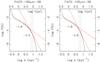 |
Fig. B.2 Same as Fig. B.1 for the degraded resolutions of 26 and 36′′. |
| In the text | |
Current usage metrics show cumulative count of Article Views (full-text article views including HTML views, PDF and ePub downloads, according to the available data) and Abstracts Views on Vision4Press platform.
Data correspond to usage on the plateform after 2015. The current usage metrics is available 48-96 hours after online publication and is updated daily on week days.
Initial download of the metrics may take a while.