| Issue |
A&A
Volume 539, March 2012
|
|
|---|---|---|
| Article Number | A121 | |
| Number of page(s) | 11 | |
| Section | Numerical methods and codes | |
| DOI | https://doi.org/10.1051/0004-6361/201118252 | |
| Published online | 05 March 2012 | |
Simulations of the solar near-surface layers with the CO5BOLD, MURaM, and Stagger codes
1 Max-Planck-Institut für Sonnensystemforschung, 37191 Katlenburg-Lindau, Germany
e-mail: This email address is being protected from spambots. You need JavaScript enabled to view it.
2 Max-Planck-Institut für Astrophysik, Karl-Schwarzschild-Str. 1, 85741 Garching, Germany
3 Leibniz-Institut für Astrophysik Potsdam (AIP), An der Sternwarte 16, 14482 Potsdam, Germany
4 Research School of Astronomy and Astrophysics, Australian National University, Cotter Rd, Weston Creek, ACT 2611, Australia
5 Centre de Recherche Astrophysique de Lyon, UMR 5574: CNRS, Université de Lyon, École Normale Supérieure de Lyon, 46 Allée d’Italie, 69364 Lyon Cedex 07, France
6 School of Physics, University of Exeter, Stocker Road, Exeter EX4 4QL, UK
7 ZAH, Landessternwarte, Königstuhl 12, 69117 Heidelberg, Germany
Received: 12 October 2011
Accepted: 16 December 2011
Abstract
Context. Radiative hydrodynamic simulations of solar and stellar surface convection have become an important tool for exploring the structure and gas dynamics in the envelopes and atmospheres of late-type stars and for improving our understanding of the formation of stellar spectra.
Aims. We quantitatively compare results from three-dimensional, radiative hydrodynamic simulations of convection near the solar surface generated with three numerical codes (CO5BOLD, MURaM, and Stagger) and different simulation setups in order to investigate the level of similarity and to cross-validate the simulations.
Methods. For all three simulations, we considered the average stratifications of various quantities (temperature, pressure, flow velocity, etc.) on surfaces of constant geometrical or optical depth, as well as their temporal and spatial fluctuations. We also compared observables, such as the spatially resolved patterns of the emerging intensity and of the vertical velocity at the solar optical surface as well as the center-to-limb variation of the continuum intensity at various wavelengths.
Results. The depth profiles of the thermodynamical quantities and of the convective velocities as well as their spatial fluctuations agree quite well. Slight deviations can be understood in terms of differences in box size, spatial resolution and in the treatment of non-gray radiative transfer between the simulations.
Conclusions. The results give confidence in the reliability of the results from comprehensive radiative hydrodynamic simulations.
Key words: radiative transfer / hydrodynamics / Sun: photosphere / convection
© ESO, 2012
1. Introduction
Comprehensive (magneto)hydrodynamic simulations have become an essential tool for studying near-surface convection in the Sun and other cool stars, together with the structure and gas dynamics in their atmospheres (e.g., Nordlund et al. 2009). These simulations attempt to include all relevant physics, such as three-dimensional (3D), time-dependent, compressible hydrodynamics, partial ionization and molecule formation as well as non-gray and non-local radiative transfer, in order to provide a “realistic” representation of the physical stratification and macroscopic gas flows in the external stellar layers. For a direct comparison with observations, spectral line profiles, continuum intensity and polarization maps are calculated on the basis of the simulation results. This comparison serves as a means of validation of the simulations and also as a tool for interpreting the observational results in terms of basic physical quantities (cf. Uitenbroek & Criscuoli 2011).
Although various codes are now being used to perform comprehensive simulations of solar and stellar (magneto)convection and an extensive body of simulation results has already been published, so far no systematic attempt has been made to cross-validate codes by quantitatively comparing numerical results. In this paper, we attempt to fill this gap, at least partially, and compare the solar models computed with CO5BOLD, MURaM, and Stagger, three independent and widely used 3D, radiative (magneto)hydrodynamic simulation codes. Apart from these codes, a number of other codes for 3D simulations of solar and stellar surface convection including (full or simplified) radiative transfer have been developed and utilized by various groups (e.g., Stein & Nordlund 1998; Robinson et al. 2003; Heinemann et al. 2006; Abbett 2007; Ustyugov 2009; Muthsam et al. 2010; Gudiksen et al. 2011).
The purpose of our study is not a comparison of the numerical approaches of CO5BOLD, MURaM, and Stagger per se, which would require using an identical setup in terms of box size, spatial resolution, and input material quantities such as opacities and equation of state. We rather wish to investigate how far simulations made for different applications are consistent in the basic properties of the simulated stellar atmosphere and uppermost convection zone. Examples of such properties are the average profiles of various quantities as a function of geometrical or optical depth. According to this rationale, we chose for comparison “standard” simulations of the near-surface layers of the Sun that were carried out by the participating groups for different purposes. The CO5BOLD and Stagger simulations provide a solar reference atmosphere (as part of a large grid of stellar models) for spectrum-synthesis calculations and abundance studies; they thus focus upon a good representation of the energy exchange by non-gray radiative transfer. The MURaM simulation, on the other hand, represents a non-magnetic comparison model for a set of magnetoconvection simulations to study fine-scale magnetic phenomena, for which high spatial resolution is crucial. The question we address here is: how much do the basic properties of the “solar models” resulting from simulations with different codes, different input quantities, different setup in terms of box size and spatial resolution, and even different top boundary conditions deviate from each other? If the differences turn out to be marginal, this result could then be taken as a kind of “cross-validation” of the codes and as a basis for confidence in the reliability of the simulations.
2. Codes
All three codes considered here treat the coupled time-dependent equations of compressible radiative (magneto)hydrodynamics and radiative transfer in a three-dimensional geometry and for a stratified, partially ionized medium. The energy exchange between radiation and matter is accounted for through solving the equation of radiative transfer under the assumption of local thermodynamic equilibrium (LTE) with a Planckian source function. To reduce the computational load, the wavelength-dependence of the radiative transfer is treated with the method of opacity binning (Nordlund 1982; Ludwig 1992; Skartlien 2000; Vögler et al. 2004). A brief overview of the numerical methods used is given in Table 1. In all cases, a local “box-in-the-star” setup is employed: the computational domain is a rectangular 3D box straddling in height the photosphere and the uppermost few Mm of the convection zone1. The simulation boxes are sufficiently extended in the horizontal directions (6–9 Mm) to contain about 15–40 convection cells (granules) at any given time, thus providing a statistically useful sample of the near-surface layers of the Sun. Periodic boundary conditions are assumed in the horizontal directions (side boundaries) while the bottom boundary is open and allows free in- and outflow of fluid. A fixed entropy density is prescribed for the inflowing fluid at the lower boundary. It can be interpreted as the entropy of the deep, almost adiabatically stratified convective envelope and controls the effective temperature of the simulated atmosphere. In addition, the gas pressure is kept constant across the bottom boundary. The three codes differ somewhat in their treatment of the upper boundary conditions, as outlined more specifically below.
Results from all three codes considered here already passed various “reality checks” by comparison with observational data (e.g., Danilovic et al. 2008; Pereira et al. 2009a,b; Wedemeyer-Böhm & Rouppe van der Voort 2009; Hirzberger et al. 2010).
2.1. CO5BOLD
The CO5BOLD code uses a numerical scheme based on a finite-volume approach on a fixed Cartesian grid. Operator splitting separates the various (usually explicit) operators: the (magneto)hydrodynamics, the tensor viscosity, the radiation transport, and optional source steps. Directional splitting reduces the multi-dimensional hydrodynamics problem to a sequence of 1D steps. The advection step is performed by an approximate Riemann solver of Roe type, modified to account for a realistic equation of state, a non-equidistant grid, and the presence of source terms due to an external gravity field. Optionally, a 3D tensor viscosity can be activated for improved stability in extreme situations. Parallelization of CO5BOLD is achieved with OpenMP.
The top boundary condition provides transmission of waves of arbitrary amplitude, including shocks: typically, two layers of ghost cells are introduced, where the velocity components and the internal energy are kept constant and the density decreases exponentially with a scale height set to a controllable fraction of the local hydrostatic pressure scale height. This gives the possibility to minimize the mean mass flux through the open top boundary.
The radiative transfer in the CO5BOLD simulation considered here was computed using a long-characteristics scheme for rays with four inclination angles and four azimuthal angles plus the vertical, i.e. 17 rays in total. The values of the inclinations (μ = cosθ = 1.000, 0.920, 0.739, 0.478, 0.165) correspond to the positive nodes of the 10th-order Lobatto quadrature formula, the four azimuthal angles coincide with the grid directions (φ = 0, π/2, π, and 3π/2). For the opacity binning, tables were constructed from a data set of MARCS raw opacities provided by Plez (priv. comm.; see also Gustafsson et al. 2008), comprising continuous and sampled atomic and molecular line opacities as functions of temperature and gas pressure at more than 105 wavelength points. The adopted chemical composition comes from Asplund et al. (2005). Each wavelength of the original opacity sampling data was sorted into one of twelve representative bins, according to wavelength and Rosseland optical depth where the monochromatic optical depth unity is reached in a 1D standard solar atmosphere. The thresholds for the opacity bins used for the present CO5BOLD solar simulation are given in Table 2. For each opacity bin, the tabulated opacity is a hybrid of Rosseland and Planck means over all frequencies of the bin, such that it approaches the Rosseland mean at high values of the optical depth, and the Planck mean at low values, with a smooth transition centered at Rosseland optical depth 0.35. Assuming LTE and pure absorption, the source function in each bin is computed as the Planck function integrated over the frequencies associated with the respective bin.
The equation of state (EOS) used in CO5BOLD follows Wolf (1983). It accounts for the partial ionization of hydrogen and helium, as well as for H2 molecule formation. In contrast to Wolf’s approach, all pressure-temperature regions are treated homogeneously since performance optimization was not necessary because a tabulated EOS is used.
The CO5BOLD simulation considered in this paper was used by Caffau et al. (2008) for the determination of the solar thorium and hafnium abundances, and for subsequent studies of CNO and other elements. More details about the CO5BOLD code can be found in Freytag et al. (2002), Wedemeyer et al. (2004), and Freytag et al. (2008, 2012).
2.2. MURaM
The MURaM code (Vögler 2003; Vögler et al. 2005) uses a 4th-order central difference scheme in space and a 4th-order Runge-Kutta scheme for time-stepping. Artificial diffusivities are treated with the scheme described in Rempel et al. (2009). An open-top boundary condition is also implemented in the MURaM code, but for the simulation considered here a stress-free, closed top (zero vertical velocity) was chosen in order to study how far this affects the mean stratification. MURaM uses the Message Passing Interface (MPI) framework for parallelization.
Radiative transfer in the MURaM code is calculated with the short-characteristics method (Kunasz & Auer 1988) with bilinear interpolation. The angular integration is carried out according to the A4 scheme of Carlson (1963) along three directions per octant, which corresponds to 12 complete rays in total (cf. Bruls et al. 1999). The opacity binning for the non-gray radiative transfer is based on the opacity distribution functions from the ATLAS9 package (Kurucz 1993) and uses 4 bins. The thresholds in optical depth (see Table 2) for the binning procedure were chosen in terms of  , which is a hybrid of the Rosseland mean in the deeper layers and the Planck mean in the upper layers, with a smooth transition centered at τ = 0.35 (Ludwig 1992; Vögler et al. 2004). The EOS tables used for the simulation considered here are based on tables from the OPAL project (Rogers et al. 1996) for a solar gas mixture with abundances from Anders & Grevesse (1989).
2.3. Stagger
The Stagger code, (originally developed by Galsgaard & Nordlund 1996) 2, uses a 6th-order finite difference scheme in space with 5th-order interpolations. Scalar variables (density, internal energy, and temperature) are volume-centered, while momenta are face-centered. The hydrodynamic variables are advanced forward in time using a 3rd-order Runge-Kutta scheme. Boundaries are periodic horizontally and open vertically, both at the top and at the bottom. The EOS is taken from Mihalas et al. (1988) and accounts for the effects of excitation, ionization, and dissociation of the 15 most abundant elements and of the H2 and H molecules. Parallelization of the Stagger code is carried out via MPI.
The radiative-transfer equation is solved with a Feautrier-like (Feautrier 1964) scheme along eight inclined rays (two inclination angles, four azimuth angles) plus the vertical, and using an opacity-binning scheme with twelve bins for the frequency dependence. The total radiative heating rate at the center of each grid cell is computed by adding the partial contributions from each direction and opacity bin with the appropriate weight. The values of the inclination angles (μ = cosθ = 0.155, 0.645, 1.000) and their associated weights (wμ = 0.376, 0.512, 0.111) correspond to the nodes and weights of the 3rd-order Radau quadrature formula; the four azimuthal angles are equidistant (φ = 0, π/2, π, and 3π/2) and have equal weights.
For the Stagger simulation considered here, the continuous opacity data came from Gustafsson et al. (1975) and Trampedach (private communication), while sampled line opacities were taken from the marcs package (Plez, priv. comm.; see also Gustafsson et al. 2008). The adopted chemical composition for the simulation considered here was taken from Asplund et al. (2005).
The opacity binning procedure implemented in the Stagger code is essentially based on the formulation by Skartlien (2000). Opacities are sorted into bins according to their wavelength and strength. As a measure of the opacity strength at a given wavelength, the Rosseland optical depth of formation of that particular wavelength is used. More precisely, the formation depth is defined as the point where the monochromatic optical depth in the vertical direction equals unity in a one-dimensional model constructed by taking the mean temperature-density stratification from a solar simulation. The thresholds in Rosseland optical depth and wavelength for the determination of bin membership are given in Table 2. Within each opacity bin, opacities are averaged and the source function contributions at the various wavelengths belonging to the bin are integrated. Mean-intensity-weighted average opacities and Rosseland-like mean opacities are adopted in the optically thin and optically thick layers, respectively. A bridging function is used for a smooth transition between the two averages near the optical surface. In the Stagger simulation considered here, the Planck function at the local temperature was chosen as the source function and the contribution of scattering to the total opacity in the optically thin layers was neglected. The simulation belongs to the series that was used in the recent analysis by Asplund et al. (2009) for the spectroscopic determination of solar abundances. A more comprehensive description of the opacity binning implementation and of the approximations involved in current Stagger code simulations are given in Collet et al. (2011).
3. Simulation runs and quantities for comparison
The three codes were used to carry out simulations of near-surface solar convection without magnetic field. As explained in the introduction, the simulation setups were different, corresponding to the different research topics that the participating groups focus upon. Therefore, the numerical setups differ in terms of (horizontal and vertical) box size, grid resolution, number of opacity bins, and other features such as the top boundary condition. In all cases, the simulation boxes include the photosphere (up to about 1 Mm above the optical surface) and the uppermost layers of the convection zone (between 1.4 Mm and 3 Mm below the optical surface, depending on the simulation). Table 3 gives various parameters of the simulation runs. Note that the Stagger code uses a non-equidistant grid of 230 cells in the vertical direction, with spacings ranging from 7 km around the optical surface and 32 km in the deepest parts of the simulation box.
The simulations were run for several hours of solar time to reach a statistically stationary, thermally relaxed state. Nineteen snapshots taken at regular intervals and spanning in total a period of about two hours were considered for the analysis of each simulation. This choice was made to ensure that the effects of the 5-min p-mode oscillations in the simulations are averaged out in the temporal means.
The physical quantities considered for the comparison are temperature, gas pressure, and turbulent pressure ( ), as well as the vertical and horizontal velocity components. To obtain mean profiles as functions of depth, z, for each of these quantities, q(xi,yj,zk,tl) ≡ qijk,l, and their squares at the grid cells (xi,yj,zk) and at time t = tl, the averages over horizontal planes (zk = const.) were determined, viz.
 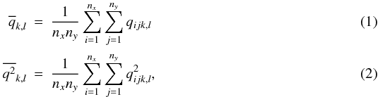 where nx and ny are the number of grid cells in the horizontal directions. Similarly, averages over surfaces of constant optical depth were determined by first calculating the optical depth along vertical lines of sight, τ500, for the continuum opacity at 500 nm wavelength and then considering the quantities at fixed levels in the range − 4 ≤ log τ500 ≤ 4. We also considered averages based on optical depth corresponding to the Rosseland mean opacity and found the results to be not significantly different from those with 500 nm continuum opacity, so that we restrict ourselves to the latter case.
From the vertical profiles  and
and  we determine temporal averages over the N = 19 snapshots considered for each simulation,
  (3)the standard deviation among the snapshots,
 ![Mathematical equation: \begin{equation} \sigma(\overline{q})_k = \left[ \frac{1}{N}\sum_{l=1}^{N} \left( \overline{q}_{k,l}-\langle \overline{q} \rangle_k \right)^2 \right]^{1/2}, \label{eq_stddev} \end{equation}](/articles/aa/full_html/2012/03/aa18252-11/aa18252-11-eq45.png) (4)and the temporal average of the spatial root-mean-square (rms) fluctuation,
(4)and the temporal average of the spatial root-mean-square (rms) fluctuation, ![Mathematical equation: \begin{equation} \langle q_{\rm rms}\rangle_k = \frac{1}{N}\sum_{l=1}^{N} \left[ \overline{q^2}_{k,l} -\left(\overline{q}_{k,l}\right)^2 \right]^{1/2}. \label{eq_rms} \end{equation}](/articles/aa/full_html/2012/03/aa18252-11/aa18252-11-eq46.png) (5)The index k in Eqs. (3–5) refers either to the geometrical depth level, zk, for averages over planes of constant geometrical depth or to the optical depth level, τ500,k, for averages over surfaces of constant optical depth. Strictly speaking, the latter averages are taken over the projections of the corrugated surfaces of constant optical depth on a horizontal plane.
(5)The index k in Eqs. (3–5) refers either to the geometrical depth level, zk, for averages over planes of constant geometrical depth or to the optical depth level, τ500,k, for averages over surfaces of constant optical depth. Strictly speaking, the latter averages are taken over the projections of the corrugated surfaces of constant optical depth on a horizontal plane.
Parameters of the simulation runs.
Global properties of the simulated solar models.
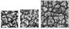 |
Fig. 1 Vertically emerging continuum intensity at 500 nm for single snapshots from the CO5BOLD (left), Stagger (middle), and MURaM (right) runs, drawn to scale. The gray scales cover, from black to white, the ranges 0.59–1.53 (CO5BOLD), 0.50–1.53 (Stagger), and 0.49–1.66 (MURaM) of the intensity normalized to the respective horizontal average. Axis units are Mm. |
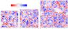 |
Fig. 2 Vertical velocity at the average geometrical depth level of the surface τ500 = 1 for the same snapshots as in Fig. 1. Downflows are shown in red, upflows in blue. The color table covers the range ± 7 km s-1 in all cases; speeds outside this range are saturated. Axis units are Mm. |
4. Results
Table 4 shows the effective temperatures of the various simulation models together with the disk-center bolometric and monochromatic continuum intensity contrasts at 500 nm. The standard deviations indicate the variability among the 19 snapshots from each simulation run used in the analysis. The effective temperatures differ by about 14 K at most and the intensity contrasts agree fairly well with each other. In comparison to the other simulations, the variations from snapshot to snapshot are smaller in the MURaM case. This is probably because of the larger horizontal extension of the computational box.
Unless stated otherwise, all quantities discussed in the following subsections refer to averages over the 19 snapshots from each of the simulation runs.
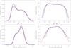 |
Fig. 3 Linear (left) and logarithmic (right) histograms of the vertically emerging continuum intensity at 500 nm (upper panels) and the vertical velocity on the average height level of the surface τ500 = 1 (lower panels) averaged over all 19 snapshots from each simulation (black: CO5BOLD, red: MURaM, blue: Stagger). Positive velocities correspond to upflows. Thirty bins were used in all cases. Each histogram was normalized such that the sum of the density function over the bins becomes unity. |
4.1. Surface maps and histograms
Figure 1 shows maps of the vertically emerging (disk-center) continuum intensity at 500 nm for snapshots from the three simulation runs. Figure 2 gives the corresponding maps of the vertical velocity at the average geometrical depth level of the surface τ500 = 1, where τ500 is the continuum optical depth at 500 nm wavelength. The runs with higher spatial resolution naturally show more small-scale details, but the basic structure and average size of the granules and the correlation between the brightness and velocity are very similar in all simulations. The visual impression is confirmed by the similarity of the histograms of intensity and vertical velocity given in Fig. 3. On a logarithmic scale (right panels), the difference in spatial resolution becomes apparent at the extreme values, but otherwise there are no significant differences between the distributions.
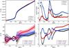 |
Fig. 4 Upper panels: horizontally averaged temperature (left) and standard deviation of the mean temperature profiles corresponding to the 19 simulation snapshots (right) as functions of geometrical depth (z = 0: average depth of τ500 = 1). Lower panels: absolute (left) and relative (right) mean temperature differences between the models. |
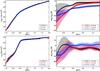 |
Fig. 5 Upper panels: horizontally averaged gas pressure (left) and relative differences between the models (right) as functions of geometrical depth. Lower panels: same for the horizontally averaged turbulent pressure, |

4.2. Mean stratification
The upper panels of Fig. 4 show the geometrical-depth profiles of the horizontally averaged temperature and their (temporal) standard deviations (see Eq. (4)), the latter indicating the level of fluctuations of the mean profiles among the 19 snapshots used from each of the three simulation runs. The depth scales of the three models were aligned such that z = 0 always refers to the average depth of the surface τ500 = 1. The weaker fluctuations between the MURaM snapshots compared to the other models are probably a result of the horizontally more extended computational box and the explicit damping of the fundamental box oscillation mode in this simulation.
The absolute and relative differences between the mean temperature profiles from the three simulations are given in the lower panels of Fig. 4. The colored bands in this plot (and in similar subsequent figures) represent the sample standard deviations3 of the differences between pairs of models on the basis of the 19 snapshots from each simulation, indicating the range of scatter caused by the temporal variability of the averages in the relatively small simulation boxes. The temperature profiles agree fairly well, with relative differences below 2% and overlapping bands of the standard deviation over most of the height range in the lower left panel of Fig. 4. The positive and negative excursions near z = 0 result from slight differences in the depth location and slope of the steep temperature gradient near optical depth unity. These differences can easily arise given the strong temperature dependence of the continuum opacity around T(τ500 = 1) ≃ 6400 K and the differing vertical resolution of the simulations. In the photosphere (−500 km ≤ z ≤ 0 km), the CO5BOLD and Stagger profiles deviate by less than 20 K from each other while the MURaM temperatures differ somewhat more, up to 60 K (i.e., at a level of about 1%).
Figure 5 shows the depth profiles of gas pressure, pgas, and of turbulent pressure,  , together with the respective relative differences between the simulations. The ratio of turbulent to gas pressure is given in Fig. 6. The turbulent pressure reaches nearly 20% of the gas pressure slightly below the optical surface (where the vertical velocity fluctuations peak) and again about this value in the top layers.
The relative differences of the gas pressure between the models are somewhat larger than those of the temperature, especially in the uppermost layers. While the roughly depth-independent deviations in the layers below z = 0 can be simply explained by a constant relative shift of the respective geometrical height scales, the bigger deviations in the photosphere are caused by the significant differences of the turbulent pressure in these layers between the simulations (cf. the lower right panel of Fig. 5). To illustrate the effect, consider the simple case of an isothermal atmosphere and constant turbulent speed, vz. The scale height of the gas pressure is then given by  , where cs is the sound speed and g is the (constant) gravitational acceleration. If the turbulent pressure differs between two stratifications, the effect is cumulative: for instance, a difference of 5% over 6 scale heights adds up to 30% of a scale height, leading to a significant pressure deviation in the upper layers. The higher turbulent speeds of the Stagger model imply a larger scale height and, therefore, higher pressure and density in the upper layers. In terms of optical depth (relevant for observations), the deviations of the pressure stratifications are significantly smaller (cf. Fig. 11) since higher values of pressure and density lead to an upward shift of the iso-τ surfaces (and vice versa).
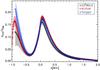 |
Fig. 6 Horizontally averaged ratio of turbulent pressure to gas pressure. |
Figure 7 shows the relative rms fluctuations of temperature and pressure, respectively, on surfaces of constant geometrical depth (see Eq. (5)). The temperature fluctuations (left panel) show a sharp maximum near the optical surface, where radiative cooling leads to strong temperature differences between granular upflows and intergranular downflow regions. The development of shocks in the uppermost layers of the simulation boxes results in a second peak of the temperature fluctuations. In contrast, the pressure fluctuations grow monotonically outward and reach their maximum at the top of the simulated regions.
The rms values of the velocity components are shown in Fig. 8. The rms of the vertical velocity (left panel) peaks near the optical surface, owing to the braking of the upflows and the acceleration of the cool downflows as a result of radiative cooling. Because the scale height decreases rapidly, most of the rising fluid that reaches the surface has to overturn very near to optical depth unity, so that the rms value of the horizontal velocity (right panel of Fig. 8) peaks only slightly higher than those of the vertical velocity. The rms of both velocity components grow again in the upper, shock-dominated top layers of the simulation boxes. The somewhat lower rms values of the CO5BOLD model are probably related to the shallower computational box in comparison to the other simulations. The drop near the bottom boundary in the case of the MURaM simulation is caused by a narrow layer of enhanced viscosity, which was introduced on grounds of numerical stability. In spite of these differences, all three codes show excellent agreement in the observable photospheric layers (−0.5 Mm < z < 0 Mm).
4.3. Photospheric structure
For all observables originating in the solar photosphere, the profiles of the physical quantities as functions of optical depth are relevant. Since the surfaces of constant optical depth are not flat but strongly corrugated in the photosphere owing to granulation, the profiles of quantities averaged over surfaces of constant optical depth generally do not simply correspond to stretched or shifted profiles of horizontally averaged quantities.
Figure 9 illustrates the relation between the geometrical and the optical depth scales. The left panel shows the mean geometrical depths of the iso-τ surfaces as a function of continuum optical depth at 500 nm. The profiles are very similar: the maximum differences between the models are on the order of the vertical distances of the grid cells. The (spatial) rms fluctuations of the depth of the iso-τ surfaces are shown in the left panel of Fig. 9. They quantify the “corrugation” of the iso-τ surfaces, which reaches a maximum of ~80 km somewhat below the optical surface, presumably because of the dominant effect of the cool downflow regions and the strong (positive) temperature dependence of the H− continuum opacity.
The profiles of temperature averaged over iso-τ surfaces and the differences between the models are shown in Fig. 10. In the photosphere, the biggest difference between the models appears in the range −1.5 < log τ500 < −0.5, where the MURaM model is up to 40 K cooler than the Stagger model and 65 K cooler (~1%) than the CO5BOLD model. This probably is a result of the less detailed opacity binning procedure used in the MURaM simulation (only 4 opacity bins compared to 12 in the other simulations). The deviation leads to a somewhat lower temperature gradient in the MURaM case between −2.5 < log τ500 < −1.5. In a narrow layer around log τ500 ≃ 0.7 below the optical surface, the MURaM model is up to 200 K hotter than the other two models. This could be related to the higher spatial resolution of the MURaM simulation, which leads to less artificial diffusion of heat between the hot upflows and cool downflows, thus maintaining bigger temperature fluctuations (cf. Fig. 12).
The profiles of gas pressure averaged over iso-τ surfaces are shown in Fig. 11. The relative differences between the models in the photosphere generally amount to a few percent. The biggest differences of up to 6.5% arise between the Stagger and MURaM models near log τ500 = −1. As explained in the preceding subsection, these differences are related to the effect of the turbulent pressure on the pressure scale height.
Figure 12 shows the spatial rms fluctuations of temperature and pressure on iso-τ surfaces. In the range −2 ≤ log τ500 ≤ 0, the horizontally averaged temperature fluctuations are similar for all models. In the higher layers, the models deviate more strongly from each other. This is a result of the differences in the velocity fluctuations and turbulent pressure discussed above.
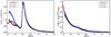 |
Fig. 7 rms fluctuations of temperature (left) and pressure (right) on surfaces of constant geometrical depth. |
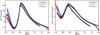 |
Fig. 8 rms of the vertical (left) and horizontal (right) velocity on surfaces of constant geometrical depth. |
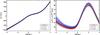 |
Fig. 9 Left: geometrical depth averaged over iso-τ surfaces (left) as functions of continuum optical depth τ500. Right: spatial rms fluctuations of the geometrical depth of the iso-τ surfaces. |
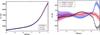 |
Fig. 10 Temperature averaged over iso-τ surfaces (left) and temperature difference between the models (right) as a function of optical depth τ500 in the photospheric layers. |
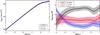 |
Fig. 11 Gas pressure profiles (left) and relative differences (right) averaged over iso-τ surfaces as functions of optical depth τ500. |
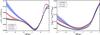 |
Fig. 12 Relative rms fluctuations of temperature (left) and pressure (right) on surfaces of constant optical depth τ500. |
The rms values of the vertical and horizontal components of the fluid velocity are shown in Fig. 13. The rms values of both components in the photosphere are very similar for all three simulations, while the deviations become somewhat larger in the layers above.
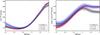 |
Fig. 13 rms of the vertical (left) and horizontal (right) velocity on surfaces of constant optical depth τ500. |
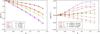 |
Fig. 14 Center-to-limb variation of the continuum intensity (left) and differences between the models (right) as a function of μ = cosθ at four wavelengths in the visible and infrared spectral ranges. |
4.4. Center-to-limb variation of continuum intensity
In order to estimate how much the differences between the models affect observable quantities, we considered the center-to-limb variation (CLV) of the monochromatic continuum intensity. The intensities were calculated at four wavelengths (400 nm, 600 nm, 800 nm, and 2000 nm) along rays with 10 inclination angles, with μ = cosθ ranging from μ = 1 (disk center) to μ = 0.1 (limb). For each inclination and wavelength, the intensities were spatially averaged over the simulated surface areas, temporarily averaged over simulation snapshots, and azimuthally averaged over four (CO5BOLD, MURaM) or 12 (Stagger) equidistant azimuthal directions.
The CLVs for the CO5BOLD simulation were computed with the spectrum synthesis code Linfor3D 4. The NLTE EOS used in Linfor3D is more detailed than that employed in CO5BOLD, because it has to provide the electron pressure and the number density for all individual atoms and ions. Likewise, the continuum opacities used in Linfor3D are not fully consistent with the raw opacities from which the binned opacities in the CO5BOLD simulations are constructed. However, both opacities are based on the same chemical abundance mix (Grevesse & Sauval 1998, with the exception of CNO, for which the values A(C) = 8.41, A(N) = 7.80, A(O) = 8.67 are adopted). The emergent continuum intensity is obtained by integrating the transfer equation on a grid that is refined with respect to the original hydrodynamics grid, ensuring that the resolution in vertical optical depth is about ΔτRoss ≈ 0.1.
The CLVs for the snapshots of the Stagger simulation were computed with the line formation code SCATE (Hayek et al. 2011), using the same Feautrier-like long-characteristics solver as in the original simulation. SCATE employs the same EOS as the Stagger code simulation and the same continuous opacities used for the opacity binning.
For the MURaM simulation, the CLVs were calculated using a long-characteristics scheme with automatic grid refinement in case of steep gradients in optical depth along the ray. It uses the same EOS as the MURaM simulation and the same continuum opacities as employed for the opacity binning (based on the opacity distribution functions from the ATLAS9 package, see Kurucz 1993). The continuum opacities are averages over 20 nm (for the CLVs at 400 nm, 600 nm, and 800 nm) or over 90 nm (for 2000 nm).
Figure 14 shows the resulting profiles for the three simulations and the differences between them. The profiles are very similar, the agreement between CO5BOLD and Stagger simulations being somewhat better (except at 400 nm) than that between MURaM and the other simulations. The somewhat stronger limb darkening mainly results from the slightly steeper temperature gradient in the lower photosphere of the MURaM model (cf. Fig. 10).
5. Conclusions
Although the three numerical solar models considered here (CO5BOLD, MURaM, and Stagger) result from codes with different numerical methods and from simulation boxes of different size and spatial grid resolution, their overall agreement is very good and encouraging. This does not only concern the mean (optical and geometrical) depth profiles of the basic quantities, but also the spatial fluctuations of these quantities as well as histograms of velocity and intensity, i.e., the dynamics and spatial structure of the simulated atmospheres. Slight deviations between the models for some quantities are probably caused by differences in spatial resolution and in the opacity binning procedures. These results give confidence in the reliability of comprehensive simulations as a tool for studying stellar atmospheres and surface convection.
However, by number of scale heights, the simulations cover about a third of the total pressure range of the convection zone.
The standard deviation of the differences is equal to the square root of the sum of the variances according to the 19 snapshots of the individual models.
Acknowledgments
B.F. acknowledges financial support from the Agence Nationale de la Recherche (ANR) and the Programme National de Physique Stellaire (PNPS) of CNRS/INSU, France. W.H. acknowledges support by the European Research Council under the European Communitys 7th Framework Programme (FP7/2007–2013 Grant Agreement no. 247060).
References
- Abbett, W. P. 2007, ApJ, 665, 1469 [Google Scholar]
- Anders, E., & Grevesse, N. 1989, Geochim. Cosmochim. Acta, 53, 197 [Google Scholar]
- Asplund, M., Grevesse, N., & Sauval, A. J. 2005, in Cosmic Abundances as Records of Stellar Evolution and Nucleosynthesis, ed. T. G. Barnes III, & F. N. Bash, ASP Conf. Ser., 336, 25 [Google Scholar]
- Asplund, M., Grevesse, N., Sauval, A. J., & Scott, P. 2009, ARA&A, 47, 481 [NASA ADS] [CrossRef] [Google Scholar]
- Bruls, J. H. M. J., Vollmöller, P., & Schüssler, M. 1999, A&A, 348, 233 [NASA ADS] [Google Scholar]
- Caffau, E., Sbordone, L., Ludwig, H.-G., et al. 2008, A&A, 483, 591 [NASA ADS] [CrossRef] [EDP Sciences] [Google Scholar]
- Carlson, B. G. 1963, in Methods in Computational Physics, ed. B. Alder, & S. Fernbach, 1, 1 [Google Scholar]
- Collet, R., Hayek, W., Asplund, M., et al. 2011, A&A, 528, A32 [NASA ADS] [CrossRef] [EDP Sciences] [Google Scholar]
- Danilovic, S., Gandorfer, A., Lagg, A., et al. 2008, A&A, 484, L17 [NASA ADS] [CrossRef] [EDP Sciences] [Google Scholar]
- Feautrier, P. 1964, SAO Special Report, 167, 80 [NASA ADS] [Google Scholar]
- Freytag, B., Steffen, M., & Dorch, B. 2002, Astron. Nachr., 323, 213 [NASA ADS] [CrossRef] [EDP Sciences] [Google Scholar]
- Freytag, B., Steffen, M., Ludwig, H.-G., & Wedemeyer-Böhm, S. 2008, Astrophysics Software Database, 36 [Google Scholar]
- Freytag, B., Steffen, M., Ludwig, H.-G., et al. 2012, J. Comp. Phys., 231, 919 [Google Scholar]
- Galsgaard, K., & Nordlund, Å. 1996, J. Geophys. Res., 1011, 13445 [NASA ADS] [CrossRef] [Google Scholar]
- Grevesse, N., & Sauval, A. J. 1998, Space Sci. Rev., 85, 161 [NASA ADS] [CrossRef] [Google Scholar]
- Gudiksen, B. V., Carlsson, M., Hansteen, V. H., et al. 2011, A&A, 531, A154 [NASA ADS] [CrossRef] [EDP Sciences] [Google Scholar]
- Gustafsson, B., Bell, R. A., Eriksson, K., & Nordlund, A. 1975, A&A, 42, 407 [NASA ADS] [Google Scholar]
- Gustafsson, B., Edvardsson, B., Eriksson, K., et al. 2008, A&A, 486, 951 [NASA ADS] [CrossRef] [EDP Sciences] [Google Scholar]
- Hayek, W., Asplund, M., Collet, R., & Nordlund, Å. 2011, A&A, 529, A158 [NASA ADS] [CrossRef] [EDP Sciences] [Google Scholar]
- Heinemann, T., Dobler, W., Nordlund, Å., & Brandenburg, A. 2006, A&A, 448, 731 [NASA ADS] [CrossRef] [EDP Sciences] [Google Scholar]
- Hirzberger, J., Feller, A., Riethmüller, T. L., et al. 2010, ApJ, 723, L154 [NASA ADS] [CrossRef] [Google Scholar]
- Kunasz, P. B., & Auer, L. 1988, J. Quant. Spectrosc. Radiat. Transf., 39, 67 [Google Scholar]
- Kurucz, R. 1993, ATLAS9 Stellar Atmosphere Programs and 2 km s-1 grid, Kurucz CD-ROM No. 13, Smithsonian Astrophysical Observatory, Cambridge, Mass./USA, 13 [Google Scholar]
- Ludwig, H.-G. 1992, Ph.D. Thesis, University of Kiel, Germany [Google Scholar]
- Mihalas, D., Däppen, W., & Hummer, D. G. 1988, ApJ, 331, 815 [NASA ADS] [CrossRef] [Google Scholar]
- Muthsam, H. J., Kupka, F., Löw-Baselli, B., et al. 2010, New A, 15, 460 [NASA ADS] [CrossRef] [Google Scholar]
- Nordlund, A. 1982, A&A, 107, 1 [NASA ADS] [Google Scholar]
- Nordlund, Å., Stein, R. F., & Asplund, M. 2009, Liv. Rev. Sol. Phys., 6, http://www.livingreviews.org/lrsp-2009-2 [Google Scholar]
- Pereira, T. M. D., Asplund, M., & Kiselman, D. 2009a, A&A, 508, 1403 [NASA ADS] [CrossRef] [EDP Sciences] [Google Scholar]
- Pereira, T. M. D., Kiselman, D., & Asplund, M. 2009b, A&A, 507, 417 [NASA ADS] [CrossRef] [EDP Sciences] [Google Scholar]
- Rempel, M., Schüssler, M., & Knölker, M. 2009, ApJ, 691, 640 [NASA ADS] [CrossRef] [Google Scholar]
- Robinson, F. J., Demarque, P., Li, L. H., et al. 2003, MNRAS, 340, 923 [NASA ADS] [CrossRef] [Google Scholar]
- Rogers, F. J., Swenson, F. J., & Iglesias, C. A. 1996, ApJ, 456, 902 [NASA ADS] [CrossRef] [Google Scholar]
- Skartlien, R. 2000, ApJ, 536, 465 [NASA ADS] [CrossRef] [Google Scholar]
- Stein, R. F., & Nordlund, A. 1998, ApJ, 499, 914 [Google Scholar]
- Uitenbroek, H., & Criscuoli, S. 2011, ApJ, 736, 69 [NASA ADS] [CrossRef] [Google Scholar]
- Ustyugov, S. D. 2009, in Solar-Stellar Dynamos as Revealed by Helio- and Asteroseismology: GONG 2008/SOHO 21, ed. M. Dikpati, T. Arentoft, I. González Hernández, C. Lindsey, & F. Hill, ASP Conf. Ser., 416, 427 [Google Scholar]
- Vögler, A. 2003, Ph.D. Thesis, University of Göttingen, Germany, http://webdoc.sub.gwdg.de/diss/2004/voegler [Google Scholar]
- Vögler, A., Bruls, J. H. M. J., & Schüssler, M. 2004, A&A, 421, 741 [NASA ADS] [CrossRef] [EDP Sciences] [Google Scholar]
- Vögler, A., Shelyag, S., Schüssler, M., et al. 2005, A&A, 429, 335 [NASA ADS] [CrossRef] [EDP Sciences] [Google Scholar]
- Wedemeyer-Böhm, S., & Rouppe van der Voort, L. 2009, A&A, 503, 225 [NASA ADS] [CrossRef] [EDP Sciences] [Google Scholar]
- Wedemeyer, S., Freytag, B., Steffen, M., Ludwig, H.-G., & Holweger, H. 2004, A&A, 414, 1121 [NASA ADS] [CrossRef] [EDP Sciences] [Google Scholar]
- Wolf, B. E. 1983, A&A, 127, 93 [NASA ADS] [Google Scholar]
All Tables
All Figures
|
Fig. 1 Vertically emerging continuum intensity at 500 nm for single snapshots from the CO5BOLD (left), Stagger (middle), and MURaM (right) runs, drawn to scale. The gray scales cover, from black to white, the ranges 0.59–1.53 (CO5BOLD), 0.50–1.53 (Stagger), and 0.49–1.66 (MURaM) of the intensity normalized to the respective horizontal average. Axis units are Mm. |
| In the text | |
|
Fig. 2 Vertical velocity at the average geometrical depth level of the surface τ500 = 1 for the same snapshots as in Fig. 1. Downflows are shown in red, upflows in blue. The color table covers the range ± 7 km s-1 in all cases; speeds outside this range are saturated. Axis units are Mm. |
| In the text | |
|
Fig. 3 Linear (left) and logarithmic (right) histograms of the vertically emerging continuum intensity at 500 nm (upper panels) and the vertical velocity on the average height level of the surface τ500 = 1 (lower panels) averaged over all 19 snapshots from each simulation (black: CO5BOLD, red: MURaM, blue: Stagger). Positive velocities correspond to upflows. Thirty bins were used in all cases. Each histogram was normalized such that the sum of the density function over the bins becomes unity. |
| In the text | |
|
Fig. 4 Upper panels: horizontally averaged temperature (left) and standard deviation of the mean temperature profiles corresponding to the 19 simulation snapshots (right) as functions of geometrical depth (z = 0: average depth of τ500 = 1). Lower panels: absolute (left) and relative (right) mean temperature differences between the models. |
| In the text | |
|
Fig. 5 Upper panels: horizontally averaged gas pressure (left) and relative differences between the models (right) as functions of geometrical depth. Lower panels: same for the horizontally averaged turbulent pressure, |
| In the text | |
|
Fig. 6 Horizontally averaged ratio of turbulent pressure to gas pressure. |
| In the text | |
|
Fig. 7 rms fluctuations of temperature (left) and pressure (right) on surfaces of constant geometrical depth. |
| In the text | |
|
Fig. 8 rms of the vertical (left) and horizontal (right) velocity on surfaces of constant geometrical depth. |
| In the text | |
|
Fig. 9 Left: geometrical depth averaged over iso-τ surfaces (left) as functions of continuum optical depth τ500. Right: spatial rms fluctuations of the geometrical depth of the iso-τ surfaces. |
| In the text | |
|
Fig. 10 Temperature averaged over iso-τ surfaces (left) and temperature difference between the models (right) as a function of optical depth τ500 in the photospheric layers. |
| In the text | |
|
Fig. 11 Gas pressure profiles (left) and relative differences (right) averaged over iso-τ surfaces as functions of optical depth τ500. |
| In the text | |
|
Fig. 12 Relative rms fluctuations of temperature (left) and pressure (right) on surfaces of constant optical depth τ500. |
| In the text | |
|
Fig. 13 rms of the vertical (left) and horizontal (right) velocity on surfaces of constant optical depth τ500. |
| In the text | |
|
Fig. 14 Center-to-limb variation of the continuum intensity (left) and differences between the models (right) as a function of μ = cosθ at four wavelengths in the visible and infrared spectral ranges. |
| In the text | |
Current usage metrics show cumulative count of Article Views (full-text article views including HTML views, PDF and ePub downloads, according to the available data) and Abstracts Views on Vision4Press platform.
Data correspond to usage on the plateform after 2015. The current usage metrics is available 48-96 hours after online publication and is updated daily on week days.
Initial download of the metrics may take a while.