| Issue |
A&A
Volume 539, March 2012
|
|
|---|---|---|
| Article Number | A60 | |
| Number of page(s) | 12 | |
| Section | Astrophysical processes | |
| DOI | https://doi.org/10.1051/0004-6361/201118071 | |
| Published online | 24 February 2012 | |
Searching for soft relativistic jets in core-collapse supernovae with the IceCube optical follow-up program
1 III. Physikalisches Institut, RWTH Aachen University, 52056 Aachen, Germany
2 Dept. of Physics and Astronomy, University of Alabama, Tuscaloosa, AL 35487, USA
3 Dept. of Physics and Astronomy, University of Alaska Anchorage, 3211 Providence Dr., Anchorage, AK 99508, USA
4 University of Michigan, Randall Laboratory of Physics, 450 Church St., Ann Arbor, MI, 48109-1040, USA
5 CTSPS, Clark-Atlanta University, Atlanta, GA 30314, USA
6 School of Physics and Center for Relativistic Astrophysics, Georgia Institute of Technology, Atlanta, GA 30332, USA
7 Dept. of Physics, Southern University, Baton Rouge, LA 70813, USA
8 Dept. of Physics, University of California, Berkeley, CA 94720, USA
9 Lawrence Berkeley National Laboratory, Berkeley, CA 94720, USA
10 Institut für Physik, Humboldt-Universität zu Berlin, 12489 Berlin, Germany
11 Fakultät für Physik & Astronomie,Ruhr-Universität Bochum, 44780 Bochum, Germany
12 Physikalisches Institut, Universität Bonn, Nussallee 12, 53115 Bonn, Germany
13 Dept. of Physics, University of the West Indies, Cave Hill Campus, Bridgetown BB11000, Barbados
14 Université Libre de Bruxelles, Science Faculty CP230, 1050 Brussels, Belgium
15 Vrije Universiteit Brussel, Dienst ELEM, B 1050 Brussels, Belgium
16 Dept. of Physics, Chiba University, 263-8522 Chiba, Japan
17 Dept. of Physics and Astronomy, University of Canterbury, Private Bag 4800, Christchurch, New Zealand
18 Dept. of Physics, University of Maryland, College Park, MD 20742, USA
19 Dept. of Physics and Center for Cosmology and Astro-Particle Physics, Ohio State University, Columbus, OH 43210, USA
20 Dept. of Astronomy, Ohio State University, Columbus, OH 43210, USA
21 Dept. of Physics, TU Dortmund University, 44221 Dortmund, Germany
22 Dept. of Physics, University of Alberta, Edmonton, Alberta, T6G 2G7, Canada
23 Dept. of Physics and Astronomy, University of Gent, 9000 Gent, Belgium
24 Max-Planck-Institut für Kernphysik, 69177 Heidelberg, Germany
25 Dept. of Physics and Astronomy, University of California, Irvine, CA 92697, USA
26 Laboratory for High Energy Physics, École Polytechnique Fédérale, 1015 Lausanne, Switzerland
27 Dept. of Physics and Astronomy, University of Kansas, Lawrence, KS 66045, USA
28 Dept. of Astronomy, University of Wisconsin, Madison, WI 53706, USA
29 Dept. of Physics, University of Wisconsin, Madison, WI 53706, USA
30 Institute of Physics, University of Mainz, Staudinger Weg 7, 55099 Mainz, Germany
31 Université de Mons, 7000 Mons, Belgium
32 Aryabhatta Research Institute of Observational Sciences (ARIES), Nainital, India
33 Bartol Research Institute and Department of Physics and Astronomy, University of Delaware, Newark, DE 19716, USA
34 Dept. of Physics, University of Oxford, 1 Keble Road, Oxford OX1 3NP, UK
35 Dept. of Physics, University of Wisconsin, River Falls, WI 54022, USA
36 Oskar Klein Centre and Dept. of Physics, Stockholm University, 10691 Stockholm, Sweden
37 Dept. of Astronomy and Astrophysics, Pennsylvania State University, University Park, PA 16802, USA
38 Dept. of Physics, Pennsylvania State University, University Park, PA 16802, USA
39 Dept. of Physics and Astronomy, Uppsala University, Box 516, 75120 Uppsala, Sweden
40 Research School of Astronomy and Astrophysics, The Australian National University, Cotter Road, Weston Creek, ACT 2611, Australia
41 Dept. of Physics, University of Wuppertal, 42119 Wuppertal, Germany
42 DESY, 15735 Zeuthen, Germany
43 Now at Dept. of Physics and Astronomy, Rutgers University, Piscataway, NJ 08854, USA
44 Now at Physics Department, South Dakota School of Mines and Technology, Rapid City, SD 57701, USA
45 Los Alamos National Laboratory, Los Alamos, NM 87545, USA
46 Also Sezione INFN, Dipartimento di Fisica, 70126, Bari, Italy
47 Now at T.U. Munich, 85748 Garching & Friedrich-Alexander Universität Erlangen-Nürnberg, 91058 Erlangen, Germany
48 Now at T.U. Munich, 85748 Garching, Germany
49 NASA Goddard Space Flight Center, Greenbelt, MD 20771, USA
Received: 12 September 2011
Accepted: 21 December 2011
Context. Transient neutrino sources such as gamma-ray bursts (GRBs) and supernovae (SNe) are hypothesized to emit bursts of high-energy neutrinos on a time-scale of ≲100 s. While GRB neutrinos would be produced in high relativistic jets, core-collapse SNe might host soft-relativistic jets, which become stalled in the outer layers of the progenitor star leading to an efficient production of high-energy neutrinos.
Aims. To increase the sensitivity to these neutrinos and identify their sources, a low-threshold optical follow-up program for neutrino multiplets detected with the IceCube observatory has been implemented.
Methods. If a neutrino multiplet, i.e. two or more neutrinos from the same direction within 100 s, is found by IceCube a trigger is sent to the Robotic Optical Transient Search Experiment, ROTSE. The 4 ROTSE telescopes immediately start an observation program of the corresponding region of the sky in order to detect an optical counterpart to the neutrino events.
Results. No statistically significant excess in the rate of neutrino multiplets has been observed and furthermore no coincidence with an optical counterpart was found.
Conclusions. The search allows, for the first time, to set stringent limits on current models predicting a high-energy neutrino flux from soft relativistic hadronic jets in core-collapse SNe. We conclude that a sub-population of SNe with typical Lorentz boost factor and jet energy of 10 and 3 × 1051 erg, respectively, does not exceed 4.2% at 90% confidence.
Key words: neutrinos / supernovae: general / gamma-ray burst: general
© ESO, 2012
1. Introduction
High-energy astrophysical neutrinos are produced in interactions of charged cosmic rays with ambient photon or baryonic fields (for reviews see Anchordoqui & Montaruli 2010; Chiarusi & Spurio 2010; Becker 2008; Lipari 2006). Acceleration of these cosmic rays to very high energies takes place in astrophysical shocks. Neutrinos escape the acceleration region and propagate through space without interaction, while nuclei are deflected in magnetic fields and no longer point back to their source (for energies below ~1020 eV). Unlike gamma-rays, neutrinos are solely produced in hadronic processes and would therefore reveal the sources of charged cosmic rays. Gamma-ray bursts (for reviews see Meszaros 2002; Zhang & Meszaros 2004) could provide the environment and the required energy to explain the production of the highest energy cosmic-rays (Waxman 1995). Recent observations indicate a connection between long GRBs (duration ≳2 s) and core-collapse supernovae (CCSNe). In several cases a GRB or X-ray flash has been observed in coincidence with an optical SN light curve implying a common physical origin: a massive stellar explosion (for a review see Woosley & Bloom 2006). Furthermore, GRBs and CCSNe were found to release a comparable amount of kinetic energy. According to the collapsar model (MacFadyen & Woosley 1999; Paczynski 1998; Woosley 1993), long GRBs have their origin in the collapse of a massive, rapidly rotating star into a black hole surrounded by an accretion disk. Relativistic jets with Lorentz boost factors of 100−1000 form along the stellar axis. The GRB-SN connection gives rise to the idea that GRBs and SNe might have the jet signature in common and a certain fraction of core-collapse SNe might host soft relativistic jets with Lorentz boost factors around 5. The Lorentz boost factor of the jet might be determined by features of the progenitor star, such as its rotation. Compared to jets in GRBs, SN jets are suggested to be equally energetic but more baryon-rich, hence they are only mildly relativistic. Such soft relativistic jets would become stalled in the outer layers of the progenitor star, leading to essentially full absorption of the electromagnetic radiation emitted by the jet and, at the same time, an efficient production of high-energy neutrinos (Razzaque et al. 2005; Ando & Beacom 2005). This motivates a search for neutrino emission, as neutrinos would be able to escape from within the star.
The IceCube neutrino detector, located at the geographic south pole, is built to detect high-energy astrophysical neutrinos (Achterberg et al. 2006). So far GRB neutrino searches have been performed offline on AMANDA (Achterberg et al. 2008, 2007b) and IceCube (Abbasi et al. 2011b, 2009b, 2010) data, triggered by gamma-ray satellite detections. Time and direction information provided by gamma-ray satellites allow an almost background free search. An untriggered search was applied to AMANDA data (Achterberg et al. 2007b), which scanned the data for a clustering of neutrinos in time. Furthermore, a dedicated search for a neutrino signal in coincidence with the observed X-ray flash of SN 2008D has been conducted by IceCube (Abbasi et al. 2011a) in order to test the soft jet scenario for CCSNe. Neither the GRB nor the SN neutrino search led to a detection yet, but set upper limits on the neutrino flux.
Early SN detections, as in the case of SN 2008D, are very rare since X-ray telescopes have a limited field of view (FoV). However, neutrino telescopes cover half of the sky at any time. If neutrinos produced in soft relativistic SN jets are detected in real time, they can be used to trigger follow-up observations (Kowalski & Mohr 2007; Ageron et al. 2012). This is realized with the optical follow-up program presented here. Complementary to the offline searches, the optical follow-up program is an online search independent of satellite detections. It is sensitive to transient objects, including those which are either gamma-ray dark or not detected by gamma-ray satellites. In addition to a gain in sensitivity, the optical observations may allow the identification of the transient neutrino source, be it a SN, GRB or any other transient phenomenon producing an optical signal. Hence, it enables us to test the plausible hypothesis of a soft relativistic SN jet and sheds light on the connection between GRBs, SNe and relativistic jets.
In order to implement the optical follow-up program an online neutrino event selection was developed for IceCube. The data are processed online by a computer farm at the south pole. A dedicated trigger selects neutrino burst candidates and the directional information is transferred to the four ROTSE telescopes, which start the follow-up immediately and continue observations for several nights. The obtained optical data are searched for a transient counterpart.
In the following, we present the optical follow-up program starting with Sect. 2, which briefly describes the expected neutrino emission according to the soft SN jet model. Section 3 outlines the IceCube component of the program while Sect. 4 focuses on the search for the optical counterpart. Finally, we discuss systematic uncertainties in Sect. 5 and show our results from the first year of data taking in Sect. 6 with a focus on the SN soft jet model. We present a first limit on the hadronic jet production in CCSNe and conclude with a summary and outlook to future extensions of the program.
2. SN neutrino flux
Motivated by the GRB-SN connection Razzaque et al. (2005) proposed a model for high-energy neutrino production in soft relativistic CCSN jets. If protons are accelerated in the jets through Fermi acceleration in internal shocks, proton-proton-collisions will produce kaons and pions. The initial formulation of the model only considered neutrino production through pion decay (Razzaque et al. 2005). It was extended by Ando & Beacom (2005, hereafter AB05), who included neutrino production from kaon decay yielding a harder and hence more easily detectable neutrino spectrum. AB05 present the calculation of the neutrino spectrum for a fixed Lorentz factor of Γ0 = 3 and a fixed jet energy of Ejet,0 = 3 × 1051 erg. In order to test a broader parameter space we calculate the neutrino flux as a function of the Lorentz boost factor Γ, the jet energy Ejet and the density, ρ, of CCSN producing a jet. In the following, we derive the neutrino flux for one SN at distance 10 Mpc assuming it hosts a jet pointing at us following the calculation of AB05.
In the AB05 model, pions and kaons are produced with 20% of the parent proton energy and follow the original E-2 energy spectrum originating from Fermi acceleration. However, protons lose energy through synchrotron radiation and inverse Compton scattering (radiative cooling) and through πp and Kp processes (hadronic cooling) causing a steepening of the spectrum at higher energies. Above a certain break energy hadronic cooling becomes dominant and steepens the spectrum by a factor E-1 while radiative cooling dominates above a second break energy resulting in a total suppression factor of E-2.
The daughter neutrino carries 25% of the pion energy or 50% of the kaon energy and its energy is related to the meson energy in the jet frame1 by  (1)AB05 assume a hadronic cooling break of 30 GeV for pions and 200 GeV for kaons. It depends strongly on the jet Lorentz factor Γ and the jet energy Ejet:
  (2)The radiative cooling break (0.1 GeV for pions and 20 GeV for kaons assumed by AB05) depends only on Γ:
  (3)Note that for certain parameter configurations the order of the two break energies can change. Finally, the proton energy reaches its maximum at the photo-pion production threshold of
  GeV, where protons interact with the dense field of 4 keV thermalized synchrotron photons. Neutrinos produced in resulting Δ + -decays are not considered by AB05. The cut-off in the proton spectrum results in a cut-off in the neutrino spectrum at
  (4)The normalization of the neutrino flux at 1 GeV scales with the jet energy.
 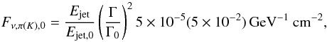 (5)where the Γ2 dependence is due to the assumed beaming with a jet opening angle of θ ∝ 1/Γ. Note that the expected number of neutrinos does not simply scale with the jet energy because the first break energy shifts with the jet energy. Depending on the choice of model parameters both the pion and kaon component of the spectrum can be hard ( ∝ E-2) or soft (∝E-3) in the energy range, which IceCube is sensitive to (TeV to PeV). Figure 1 illustrates the behavior of the total neutrino spectrum (sum of pion and kaon component) for different jet energies and Lorentz boost factors.
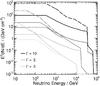 |
Fig. 1 SN neutrino spectrum according to AB05 for one SN at distance 10 Mpc with the jet pointing to us. Different shades of gray indicate different Lorentz boost factors. Solid lines: Ejet = 3 × 1051 erg. Dotted line: Ejet = 0.3 × 1051 erg. Dashed line: Ejet = 30 × 1051 erg. |
3. IceCube
The IceCube neutrino telescope has been under construction at the geographic south pole since 2004 and was completed in the Antarctic summer of 2010/11. It is capable of detecting high energy neutrinos with energies of  GeV and is most sensitive to muon neutrinos with energies in the TeV range and above. High-energy muon neutrinos undergoing charged current interactions in the ice or the underlying rock produce muons in neutrino-nucleon interactions. The muon travels in a direction close to that of the neutrino and emits Cherenkov light, which is detected by a three dimensional array of light sensors. For this purpose, a volume of 1 km3 of clear ice in depths between 1450 and 2450 m below the ice surface was instrumented with 5160 digital optical modules (DOMs) attached to 86 vertical strings (Achterberg et al. 2006). Each DOM consists of a 25 cm diameter Hamamatsu photomultiplier tube (PMT) and supporting hardware inside a pressure glass sphere (Abbasi et al. 2009a). The detector consists of 78 strings arranged in a hexagonal shape with a string spacing of 125 m and DOMs separated vertically by 17 m, and 8 strings composing the low-energy extension DeepCore (Abbasi et al. 2011e), a densely spaced array in the bottom half of the detector. The observatory also includes a surface array, IceTop, to measure properties of extensive air showers and study the composition and spectrum of cosmic rays (Stanev 2009). Figure 2 shows a top view of the IceCube detector including DeepCore. Different colors/symbols indicate different deployment stages. Before completion of the full detector, IceCube took data with the available number of strings. The optical follow-up program has been fully operational since Dec. 16, 2008. Here, we present the analysis of the data taken from Dec. 16, 2008 to Dec. 31, 2009. Initially, 40 IceCube strings were taking data (yellow upward-pointing triangle, green diamonds, red squares and magenta stars in Fig. 2). In May 2009, additional 19 strings were included (strings marked by purple downward-pointing triangles in Fig. 2 including the first DeepCore string marked by an open downward-pointing triangle). In the following, these deployment stages will be referred to as IC 40 and IC 59, respectively.
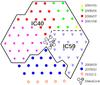 |
Fig. 2 The IceCube detector: The full detector consists of 86 strings with 60 DOMs attached to each string. Different colors/symbols indicate different deployment stages. The solid black line encircles the IC 59 configuration, while the dashed line indicates the smaller IC 40 configuration. |
To suppress the background caused by PMT noise or radioactive decay in the glass, a total number of eight DOMs with coincident hits in a time window of 5 μs are required for a trigger to be formed. A coincident hit is registered when a single DOM and its neighbor or next-to-neighbor DOM on the same string exceed their charge threshold of 0.25 photoelectrons within a time window of 1 μs. If the detector is triggered the information of all triggered DOMs within a readout window starting 10 μs before the first hit and ending 10 μs after the last hit is read out and merged to an event. Overlapping readout windows are merged together. The waveform of the PMT is digitized and sent to the surface. The waveforms have a length of up to 6.4 μs and can contain multiple hits. The total number of photoelectrons and their arrival times are extracted with an iterative unfolding algorithm.
The arrival time of the Cherenkov photons can be measured with an accuracy of ~3.3 ns (Abbasi et al. 2009a). Several hit DOMs allow a reconstruction of the direction of muon-neutrinos with a precision of ~1°. To reduce the contribution from noise, only hits within a 6 μs time window are used for the reconstruction (time window cleaning). This time window is defined as the window that contains the most hits during the event. Muons travel along a straight path through the detector while electrons or taus produce showers (cascades). Only the muon signature allows an accurate reconstruction of the direction. Directional information is crucial in order to provide coordinates for optical telescopes and we therefore consider only muon neutrino events.
3.1. Online system
In order to rapidly trigger optical telescopes, the first online analysis of high-energy neutrino events in IceCube was implemented. Unlike for the offline analyses, which are performed on an entire dataset (usually ~1 year of data) with time consuming reconstructions on a large computer cluster, the data are processed online by a computer cluster at the south pole. During IC 40 (IC 59) data taking, the cluster consisted of approximately 60 (100) processing nodes. The processing includes event reconstruction and basic event selection. Several filters and reconstruction algorithms run on the cluster (see Sect. 3.3 for details on the filters and reconstructions). During IC 40 and IC 59 events were read from the data acquisition and written to files with each file containing about 1 GB of data. The data volume of 1 GB corresponds to a data taking period of ~5 min or ~4 × 10⁵ events for IC 40. Due to larger event sizes the same volume relates to ~2.5 min or ~2.5 × 10⁵ events in IC 59. The files were then distributed to the processing nodes. Each file has to be processed by a single node. Although the processing time of ~35 ms per event is fast, the processing time per file amounts to ~4 h in IC 40 and to ~2.5 h in IC 59. For technical reasons, an additional latency of 4 h was added to ensure correct ordering of the data after processing, which results in a total latency of 6.5−8 h2. The processed and ordered data arrive on a dedicated machine (the analysis client), which is not part of the parallel processing. There, a sophisticated event selection is applied based on the reconstructed event parameters. A multiplet trigger selects candidates of neutrino clusters, which are coincident in time and space. No further reconstruction algorithms need to be applied allowing a very fast filtering of the events. If a multiplet is found, its directional information is transferred to Madison, Wisconsin, via the Iridium satellite network within ≲ 10 s. From there, the message is forwarded to the four ROTSE telescopes via the Internet through a TCP-socket connection for immediate follow-up observations. The stability and performance of the online system is constantly monitored in order to allow for a fast discovery of problems. To achieve this, test alerts are produced at a much higher rate (~100 test alerts per day compared to 25 real alerts per year) by the same pipeline and are also sent to the North. Their rate and delay time distributions are monitored using an automatically generated web page. If the rate deviates significantly from the expected, a notification is issued.
3.2. Neutrino dataset
We present the analysis of data taken from Dec. 16, 2008 to Dec. 31, 2009. This corresponds to a lifetime of 121 days with IC 40 and 186.4 days with IC 59. Dead time is predominantly caused by calibration and commissioning runs during and after the construction season. The downtime of the online system amounts to 6.8% mainly caused by downtime of the satellite transmission system.
The background in a search for muon-neutrinos of astrophysical origin can be divided into two classes. One consists of atmospheric muons, created in meson decays in cosmic ray air showers, entering the detector from above. The other background is atmospheric neutrinos which originate in the same meson decays in cosmic ray air showers. Both are measured with IceCube and are well understood: the measurement of the atmospheric neutrino spectrum with IceCube in its 40-string configuration is discussed in Abbasi et al. (2011c), the atmospheric muon energy spectrum measured with the 22-string configuration is presented in Berghaus (2009). The flux of atmospheric muons exceeds the flux of atmospheric neutrinos by 5 orders of magnitude. The background of atmospheric muons can be reduced significantly by restricting the neutrino search to the northern hemisphere. Muons from the northern hemisphere cannot penetrate the Earth and reach the detector. However, a small fraction of the southern hemisphere muons are mis-reconstructed, i.e. truly down-going (entering the detector from above) but reconstructed as up-going. Owing to the large flux of atmospheric muons, these mis-reconstructed muons represent a significant contamination. Imposing requirements on the event reconstruction quality allows a suppression of the mis-reconstructed muon background.
3.3. Neutrino selection criteria and efficiency
The expected neutrino signal according to the soft jet SN model can be calculated as a function of two model parameters: the Lorentz boost factor Γ and the jet energy Ejet (see Sect. 2). Signal events are simulated following the predicted neutrino flux spectrum in order to develop and optimize selection criteria to distinguish signal and background events. To suppress the background of atmospheric neutrinos, which we cannot distinguish from the soft SN neutrino spectrum, we require the detection of at least two events within Δt = 100 s and an angular difference between their two reconstructed directions of ΔΨ ≤ 4°. The choice of the size of the time window is motivated by the duration of the jet, i.e. the activity of the central engine, which is typically 10 s (Razzaque et al. 2005). The observed gamma-ray emission from long GRBs has a typical length of 50 s (Gehrels et al. 2009), which roughly corresponds to the time for a highly relativistic jet to penetrate the stellar envelope. The angular window ΔΨ is determined by the angular resolution of IceCube and was optimized along with the other selection parameters. The final set of selection cuts has been optimized in order to reach a background multiplet rate of ~25 per year corresponding to the maximal number of alerts accepted by ROTSE. Combining the neutrino measurement with the optical measurement allows the cuts to be relaxed compared to the neutrino point source analysis with IceCube (Abbasi et al. 2011d) yielding a larger background contamination but at the same time a higher signal passing rate.
One doublet is not significant by itself, but may become significant when the optical information is added. From the maximal allowed background multiplet rate a corresponding maximal singlet rate R1 can be estimated as follows. The probability to obtain a background triplet (three atmospheric neutrinos arriving by accident within 100 s and within ΔΨ) or any multiplet of higher order is negligible, we therefore only consider doublets. Requiring no more than 25 background doublets per year (R2 ≲ 25 year-1) corresponds to a rate of isotropic background singlets of: 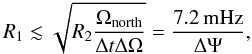 (6)where ΔΩ = π(ΔΨ)2 is the solid angle defined by the doublet condition and ΩNorth = 20627(°)2 is the solid angle of the Northern sky, i.e. 2π. The event selection is optimized in order to restrict the singlet rate to 7.2 mHz/ΔΨ while obtaining the best signal passing rate. ΔΨ = 4° was found to be the best choice during the cut optimization. This corresponds to a singlet rate of 1.8 mHz. The event selection is based on one of the standard IceCube muon event filters (in the following referred to as Level 1), which is commonly used by several offline analysis. It is discussed in detail in Abbasi et al. (2011d). The Level 1 filter selects muon tracks, which are reconstructed as up-going (passing through the Earth) based on fast and simple algorithms. It selects ~2% of all triggers with a signal efficiency of 90% for up-going neutrinos following an E-2-spectrum. It is still largely dominated by atmospheric muons. To the Level 1 filter stream we apply additional selection criteria mainly based on the reconstruction quality. This yields the so-called Level 2 filter stream. The significantly smaller rate of ~3 Hz allows us to perform time consuming reconstructions online, which provide a more accurate estimate of the event direction. These reconstructions are based on a muon-likelihood function described in Ahrens et al. (2004), which parametrizes the probability of observing the spatial distribution and timing of the hits with respect to a muon track hypothesis. The negative logarithm of the likelihood, − log ℒ, is minimized, i.e. the likelihood, ℒ, is maximized by varying the track direction to yield the best-fit direction and position for the muon track. Iterative fits repeat the minimization with a different initial track hypothesis to reduce the problem of local minima. The iteration with the smallest minimum is the final fit result. At Level 2, a ten-fold iterative likelihood reconstruction is available. The uncertainty on the reconstructed direction, σ, is obtained from a fit of a paraboloid to the − log ℒ space around the direction. Based on these more sophisticated reconstruction algorithms we select our final event stream, Level 3: a powerful parameter to reject mis-reconstructed events is given by the reduced negative logarithm of the likelihood, − log ℒ/(NCh − 5) or a modified version given by − log ℒ/(NCh − 2) or − log ℒ/(NCh − 3.5), where NCh is the number of triggered DOMs after time window cleaning.
A large number of hits with a small time residual, NDir, i.e. registered within a time window [− 25 ns, 75 ns] relative to the expected arrival time for unscattered light given by the track geometry, ensures a good track reconstruction quality, since photons causing those direct hits are less affected by scattering. Furthermore, the maximum distance, LDir, along the reconstructed track direction between any two hits with small time residual ([− 25 ns, 75 ns]) is a measure of the track quality. In addition, only up-going events with zenith angle θ ≥ 85° (IC 40) and θ ≥ 90° (IC 59) are selected3. In IC 40, an additional cut on the doublet direction was applied selecting only doublets with a combined zenith of θDoublet ≥ 90°. A single-iteration likelihood reconstruction (llh1) and a second two-iteration likelihood reconstruction (llh2) using the seed track and the inverted seed track of llh1 were used in IC 40. The ten-fold iterative likelihood reconstruction (10it) was used in both IC 40 and IC 59.
The final cuts at Level 3 for IC 40 are  and for IC 59
 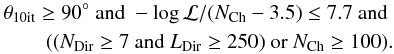 The spectrum obtained from the AB05 model can be either hard or soft depending on the choice of model parameters. The choice of cuts specified above is a compromise yielding adequate passing rates for all considered model parameters. Figure 3 shows the energy dependence of the Level 3 filter efficiency relative to Level 2 for well-reconstructed events (
 and θtrue > 90°, where the unit vector
  indicates the track direction). The filter efficiency is defined as the fraction of simulated signal events passing the filter. For energies above 100 TeV the filter is 90% efficient while for lower energies the efficiency decreases to 50% at 1 TeV and 20% at 100 GeV.
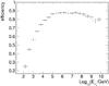 |
Fig. 3 Filter efficiency of Level 3 relative to Level 2 as function of energy for well-reconstructed events (IC 59). |
The cuts were adjusted from IC 40 to IC 59 to account for the larger detector volume in order to obtain a similar data passing rate. Table 1 shows the data passing rates for IC 40 and IC 59 at different cut levels. Furthermore, the table contains the expected number of detected SN neutrinos for a SN at distance dSN = 10 Mpc with a jet of energy Ejet = 3 × 1051 erg, which points towards Earth, and two choices of the boost factor Γ (4 and 10). The expected number of well-reconstructed SN neutrinos is given in brackets since only these events are useful to trigger optical telescopes. Figure 4 shows the expected number of events for different model parameter configurations for IC 59.
 |
Fig. 4 Expected number of SN neutrinos from a SN at distance 10 Mpc with a jet pointing towards Earth for different model parameter combinations (IC 59). |
Cut levels and event rates.
Table 1 shows that we expect many more neutrino events for a SN with a high boost factor. On the other hand, a large boost factor implies a small jet opening angle (θ ∝ 1/Γ) and hence a smaller probability of the jet pointing towards Earth. Furthermore, one sees an increase in the expected number of SN neutrinos at Level 3 from IC 40 to IC 59. The detector volume increased by roughly 50%. However, owing to improved performance of the reconstruction algorithms applied to data of the larger IC 59 detector, the signal passing rate at Level 3 increased by 52% (Γ = 10) and 68% (Γ = 4). The increase for well-reconstructed events is even higher (71% for Γ = 10 and 87% for Γ = 4). The neutrino effective area for well-reconstructed events at final cut level is shown in Fig. 5 for IC 40 and IC 59.
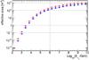 |
Fig. 5 Neutrino effective area at the final selection level for well-reconstructed events for IC 40 (blue squares) and IC 59 (red circles). |
The Level 3 cuts reduce the singlet rate to ~1.8 mHz for IC 59. The IC 40 rate is slightly higher at 2.2 mHz, but an additional cut on the doublet direction (θdoublet ≤ 90°) ensures a multiplet rate of less than 25 per year. The Level 3 data stream consists of 37% (70%) atmospheric neutrinos for IC 40 (IC 59), the rest is a contamination of mis-reconstructed atmospheric muons. In addition – as described above – we require at least two events to arrive within Δt = 100 s and with an angular distance of ΔΨ ≤ 4° to reduce the background of atmospheric neutrinos. The signal efficiency of the angular coincidence cut for different zenith bands is displayed in Fig. 6.
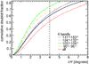 |
Fig. 6 Angular difference between the reconstructed directions of two neutrinos with identical true direction for jet parameters Γ = 3 and Ejet = 3 × 1051 erg (IC 59). |
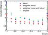 |
Fig. 7 Doublet resolution using an ordinary mean (blue circles), a weighted mean (red squares) compared to the singlet resolution (green triangles) for signal neutrinos (Γ = 3, Ejet = 3 × 1051 erg). Applying the directional coincidence cut ΔΨ < 4° (black triangles) keeps mainly well-reconstructed doublets and yields a further improvement of the doublet resolution (IC 59). |
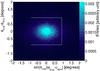 |
Fig. 8 Deviation of reconstructed multiplet direction from true direction (IC 59). The black box shows ROTSE’s field of view of 1.85° × 1.85°. |
The average passing rates depend on the assumed energy spectrum (i.e. the model parameters) and are in the range of 56−69% (IC 40) and 60−74% (IC 59) for 1 ≤ Γ ≤ 10 and 3.1 × 1049 erg ≤ Ejet ≤ 3 × 1053 erg. The reconstruction accuracy has improved because of the increased detector volume. Large reconstruction uncertainties might lead to mis-pointing of the telescopes and in the worst case the real source position might lie outside ROTSE’s field of view of 1.85° × 1.85°. To improve the accuracy of the direction forwarded to the telescopes, the doublet direction is calculated as a weighted mean from the directions of the individual events in the multiplet. The single events are weighted with 1/σ2, where σ is the reconstruction error estimated by the paraboloid fit. Compared to single events, doublets have a better resolution. The weighting improves the doublet resolution as can be seen in Fig. 7. It further improves after applying the directional coincidence condition ΔΨ ≤ 4°. Figure 8 shows the doublet point spread function in θ-φ-space compared to ROTSE’s FoV. Depending on the model parameters, 41–53% (IC 40) and 44–61% (IC 59) of all doublet events lie within ROTSE’s field of view, providing a good match for this search.
4. Search for optical counterparts
The IceCube multiplet alerts are forwarded to the robotic optical transient search experiment (ROTSE), which consists of four identical telescopes located in Australia, Texas, Namibia and Turkey (Akerlof et al. 2003). The telescopes stand out because of their large FoV of 1.85° × 1.85° and a rapid response with a typical telescope slew time of 4 s to move the telescope from the standby to the desired position. The telescopes have a parabolic primary mirror with a diameter of 45 cm. To be sensitive to weak sources no bandwidth filter is used. ROTSE is most sensitive in the R-band (~650 nm). The wide field of view is imaged onto a back-illuminated thinned CCD with 2048 × 2048 13.5 μm pixels. The camera has a fast readout cycle of 6 s and is cooled to − 40° C in order to reduce thermal noise. For a 60 s exposure at optimal conditions the limiting magnitude is around mR ≈ 18.5, which is well suited for a study of GRB afterglows during the first hour (up to one day for very bright afterglows) and SN light curves with apparent peak magnitude ≤ 16.
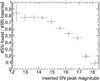 |
Fig. 9 Efficiency to find inserted SNe as a function of the apparent peak magnitude averaged over all alert directions assuming a template light curve. |
The corresponding FWHM (full width at half maximum) of the stellar images is <2.5 pixels (8.1 arcsec). The telescopes are operated robotically and managed by a fully-automated system. Observations are scheduled in a queue and are processed in the order of their assigned priority. IceCube triggers have second highest priority after GRB follow-ups triggered by the GRB Coordinate Network (GCN).
Once an IceCube alert is received by one of the telescopes, a predefined observation program is started and the corresponding region of the night sky will be observed within seconds: the prompt observation includes thirty exposures of 60 s length, follow-up observations are performed for 14 nights. This was extended on Oct. 27, 2009 to 24 nights, with daily observations for 12 nights and then observations during every second night up to day 24 after the trigger was received. Eight images with 60 s exposure time are taken per night. The prompt observation is motivated by the typical rapidly decaying light curve of a GRB afterglow, while the follow-up observations during 14 or 24 nights permit the identification of a rising SN light curve. With IC 40 and IC 59, the online processing latency of several hours made the search for an optical GRB afterglow unfeasible. We therefore focus on the SN light curve detection in the ROTSE data.
Image correction and calibration are performed at the telescope sites. The images of each night are co-added in order to obtain a deeper image. Co-adding includes a geometrical transformation to correct for optical distortions and mis-alignment of the images before the pixel contents are added. A reference image is subtracted from each co-added image. As deep images are usually not available for the positions we would like to observe, we initially choose the deepest image of our observing sequence as the reference image (due to different weather conditions in different nights the image quality varies). The source could be present in the reference image, but it would be of different brightness compared to earlier or later images, and both positive and negative deviating sources in the subtracted images will be detected. If no early image of good quality was available to be selected as reference image (30% of the alerts) we take another deep image several months later. Both SN light curves and GRB afterglows would have faded after a few weeks and would not be present in the newly taken reference image.
The applied subtraction algorithm was developed by Yuan & Akerlof (2008). Both the new and the reference image are folded by a kernel function in order to match their point spread functions (PSFs). The convoluted images then allow a pixel by pixel subtraction. The software SExtractor (source extractor), Bertin & Arnouts (1996), extracts all objects from an image by first determining the background and then identifying clusters of pixels with a significance >1σ above the background level. All extracted objects found in the subtracted images with signal-to-noise ratio larger than 5 are candidates for variable sources. However, bad image quality, failed image convolution, bad pixels and other effects frequently cause artifacts in the subtraction process, requiring further selection of the candidates. A candidate identification algorithm including a boosted decision tree is applied to classify candidates according to geometrical and variability criteria. The algorithm was trained using a signal of a SN light curve starting at the time of neutrino detection. We use a SNIbc template light curve based on SN1999ex (Hamuy et al. 2002). The time of the shock break-out was measured for SN1999ex and provides a time stamp for the explosion, i.e. the start of the light curve, which can be associated with high-energy neutrino emission. To simulate the SN, fake stars are inserted on top of galaxies in every single image from the observation sequence with a brightness according to the SN light curve template. To ensure that the PSF of the inserted star reflects all the features of the PSF of existing stars in the image we use the mean PSF of all stars in a 291 × 291 pixel box around the insertion coordinates. The PSF of a single star is obtained from a box of 15 × 15 pixel around the star’s center. The manipulated images are processed with the same pipeline as described above. The signal sample consisting of inserted fake SNe is used to train the classification algorithm as well as to estimate ROTSE’s efficiency. The efficiency is given by the fraction of inserted SNe, that has been detected by the processing and candidate identification. For some inserted SNe the detection algorithm fails: If the quality of the image is bad (e.g. large average FWHM or small limiting magnitude) the image convolution performs badly. Candidates close to saturated objects or close to objects listed in the two micron all sky survey (2MASS) point source catalog, which are very likely stars, are removed automatically. Figure 9 shows the fraction of simulated SNe that are found by the algorithm as a function of the inserted apparent peak magnitude. The efficiency as a function of the apparent peak magnitude can be converted to the efficiency as a function of SN distance εROTSE(d) (see Fig. 10) assuming an absolute R-band magnitude of M = −18 ± 1 for core-collapse SNe (Richardson et al. 2006). The relation of distance and magnitude is given by 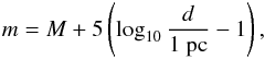 (7)where m is the apparent magnitude.
The efficiency is used to calculate the number of expected SNe detections for a given signal neutrino hypothesis. However, it may also be used to estimate, for a given SN rate, the number of accidental coincidences between a neutrino doublet and a SN detectable by ROTSE (see Sect. 6).
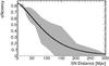 |
Fig. 10 Black curve: efficiency to detect core-collapse SN as a function of the distance to the SN assuming an absolute R-band magnitude of − 18 ± 1. Shaded region: lower bound assuming an absolute magnitude of − 17, upper bound assuming − 19. The breaks in the shaded regions are connected to the binning in Fig. 9. The binning effect is washed out in the black curve due to the assumed uncertainty in the absolute magnitude distribution of ± 1. |
After application of the classification algorithm ~10−200 candidates for variable objects remain per alert depending on the quality of the images and the Galactic latitude. Fields close to the Galactic plane contain a large number of stars, which complicates the subtraction and thus results in more candidates caused by subtraction artifacts. Tightening the cuts would reduce the number of candidates but at the same time reduce our sensitivity. The final candidates are summarized on a web page and are inspected visually by people trained on the signal simulation. The web page shows a 100 × 100 (pixel) extract of the new, the reference and the subtracted image for each night. For comparison, an image from the digitized sky survey (DSS4) of the same patch of the sky is shown, which is deeper than the ROTSE images. In addition, links to catalogs, such as NED5, 2MASS (Skrutskie et al. 2006) and SDSS (Adelman-McCarthy et al. 2008) are provided. On the basis of this information the scanners have to decide whether the candidate is a SN, a variable star or a subtraction artifact. SN candidate identification by the human eye works well as shown in the galaxy zoo SN project (Smith et al. 2010). The visual scanning of the final candidates was carried out by three individual persons, who obtained similar results. All simulated SNe, which passed the computer selection, were identified in the scanning, i.e. the efficiency was 100%. Also the rate of false positives is expected to be small, because for a potential SN candidate its light curve and host galaxy properties would be inspected in detail. We hence assume, that the systematic uncertainty introduced by the scanning process is negligible. Note that in the future, for candidates identified in real time a spectrum can be obtained to ensure an unambiguous identification of the SN.
5. Systematic uncertainties
Both the simulated neutrino sensitivity and the SN sensitivity are subject to systematic uncertainties. These systematic uncertainties are included in the limit calculation. In this limit calculation, Monte Carlo experiments are performed drawing the number of signal neutrino-events following a Poisson distribution (see appendix A for details on the limit calculation). Systematic uncertainties are included by smearing the Poisson mean, i.e. the Poisson mean is multiplied by a factor following a Gaussian distribution with mean one and a width given by the systematic uncertainty.
5.1. Systematic uncertainties on the neutrino event rate
The main sources of systematic uncertainties arise in the description of the DOM efficiency and the photon propagation in ice. The systematic uncertainties due to photon propagation are evaluated by performing dedicated simulations with scattering and absorption coefficients varied within their uncertainties of ~10% (Ackermann et al. 2006). The maximum difference was found between the case where both scattering and absorption were increased by 10% and the case where both were decreased by 10%. Varying the DOM efficiency resulted in a variation of the event rate of up to 18%. The neutrino cross section used in the neutrino simulation is based on CTEQ5 measurements, which are not up-to-date anymore. The latest cross section calculation by Cooper-Sarkar & Sarkar (2008) differ from the cross sections used in the IceCube neutrino simulation by up to 10% in the relevant energy regime. To first order, the neutrino rate depends linearly on the cross section. Folding the expected SN neutrino spectrum with an energy dependent correction factor allows us to calculate the effect on the neutrino event rate, which is up to 6%.
Finally, the uncertainty in the muon energy loss amounts to 1%, resulting in a 1% influence on the event rate (Achterberg et al. 2007a). The systematic uncertainties are energy dependent and the SN neutrino spectrum varies with the model parameters. Therefore, we calculate the quadratic sum of all listed systematic uncertainties for each combination of model parameters (see Fig. 11).
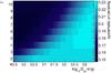 |
Fig. 11 Systematic uncertainties (relative to the predicted SN neutrino event rate) depending on model parameters Γ and Ejet. |
Table 2 summarizes the systematic uncertainties considered in this analysis and their influence on the event rate for those model parameters, where the effect is largest.
Systematic uncertainties and their influence on the event rates.
5.2. Systematic uncertainties on the SN sensitivity
The number of expected observed SNe depends on the sensitivity of the telescopes. The estimate described in Sect. 4 yields the efficiency as a function of the SN peak magnitude. The photometric zero-points as determined from USNO A2.0 R-band magnitudes have typical systematic uncertainties of up to 0.30 mag (Rykoff et al. 2005, and references therein). Shifting the efficiency curve by ±0.3 mag results in a variation of the expected number of SNe measured by ROTSE of [−17.6%, +26.6%] .
The expected number of accidentally found SNe depends on the overall core-collapse SN rate, which is assumed to be 1 SN per year within a sphere of radius 10 Mpc (continuum limit from Ando et al. 2005). The true SN rate might be higher since nearby SNe surveys tend not to target small galaxies. During the last decade 17 SNe within 10 Mpc were observed (Kistler et al. 2011). We assume a systematic uncertainty of 30% due to inhomogeneity of the local universe and 30% on the CCSN rate. Systematic uncertainty introduced by the scanning process are considered negligible.
Systematic uncertainties.
6. Results
This paper presents the results from the analysis of data taking in the period of Dec. 16, 2008 to Dec. 31, 2009. IceCube was running initially in the IC 40 configuration (Dec. 16, 2008 to May 20, 2009) and later in the IC 59 configuration (May 20, 2009 to Dec. 31, 2009)6. Table 4 shows the number of detected and expected doublets and triplets for the IC 40 and the IC 59 datasets as well as the number of detected and expected optical SN counterparts. The IceCube expectation based on a background-only hypothesis was obtained from scrambled datasets. To correctly incorporate detector asymmetries, seasonal variations and up-time gaps, we used the entire IC 40 and IC 59 datasets and exchanged the event directions randomly while keeping the event times fixed. For each scrambled dataset we obtain the number of doublets by comparing event directions. The number of doublets in both datasets (IC 40 and IC 59) shows a small excess, which corresponds to a 2.1σ effect and is thus not statistically significant.
Measured and expected number of multiplets.
To estimate the expected number of randomly coincident SN detections, we assume a core-collapse SN rate of 1 per year within a sphere of radius 10 Mpc, i.e. 2.4 × 10⁻⁴ y-1 Mpc-3, and a Gaussian absolute magnitude distribution with mean of −18 mag and standard deviation of 1 mag (Richardson et al. 2006). Based on the efficiency estimated in Sect. 4 we can calculate the rate of core-collapse SNe that could be detected by ROTSE, if it would continuously survey the full sky,  y-1. For this we integrated the CCSN rate over the accessible volume weighted with the efficiency displayed in Fig. 10. The number of expected accidental SN detections (i.e. a SN detection in coincidence with a background neutrino multiplet) is
 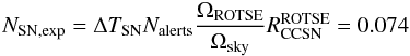 (8)where Nalerts = 17 is the number of multiplet alerts followed-up by ROTSE, ΩROTSE = 1.85° × 1.85° is the solid angle covered by ROTSE’s field of view and Ωsky = 41 253(°)2 is the all sky solid angle. ΔTSN is the time window in which we accept a coincidence of neutrino and optical signals. It has to be larger than the uncertainty of the SN explosion time. In Cowen et al. (2010) it is shown, that the explosion time can be estimated with an accuracy of ~1 day if early data are available. We choose to be conservative and take ΔTSN = 5 days. In total, 31 alerts were forwarded to the ROTSE telescopes. Five could not be observed because they were too close to the Sun. For two alerts no good data could be collected. Seven alerts were discarded because the corresponding fields were too close to the Galactic plane and hence too crowded. Thus 17 good optical datasets remained for the analysis. The data were processed as described above. No optical SN counterpart was found in the data. We calculate the limit on the AB05 model parameters following the description in Appendix A for the jet Lorentz boost factors Γ = 6,8,10 and in each case vary the jet energy Ejet and the rate of SNe with jets ρ. The algorithm was formulated prior to the start of the program. The systematic uncertainties discussed in Sect. 5 are included in the limit calculation. For each Γ-value the 90% confidence region in the Ejet-ρ-plane is displayed in Fig. 12.
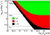 |
Fig. 12 Limits on the choked jet SN model Ando & Beacom (2005) for different Lorentz boost factors Γ as a function of the rate of SNe with jets ρ and the jet energy Ejet. The colored regions are excluded at 90% confidence level. Horizontal dashed lines indicate a fraction of SNe with jets of 100%, 10% or 1% (relative to an assumed CCSN rate of 1 per year within a sphere of radius 10 Mpc). |
The colored regions are excluded with 90% confidence. The limits include the optical information, i.e. that no optical counterpart was found. This improved the limit and allows tests of 5–25% smaller CCSN rates. The largest improvement is obtained for small jet energies and large CCSN rates. The most stringent limit can be set for high Lorentz factors, while for small Γ the constraints are weak. At 90% confidence level, a sub-population of SNe with typical values of Γ and Ejet of 10 and 3 × 1051 erg, respectively, does not exceed 4.2%. This is the first limit on CCSN jets using neutrino information.
7. Summary and outlook
This first analysis, using the four ROTSE telescopes, proves the feasibility of the program for follow-up observations triggered by neutrino multiplets detected by IceCube. The technical challenge of analyzing neutrino data in real time at the remote location of the south pole and triggering optical telescopes has been solved. First meaningful limits to the SN slow-jet hypothesis could be derived already after the first year of operation. Especially in cases of high Lorentz boost factors of Γ = 10 stringent limits on the soft jet SN model are obtained. Soderberg et al. (2010) obtain an estimate on the fraction of SNe harboring a central engine, which powers a relativistic outflow, from a radio survey of type Ibc SNe. They conclude that the rate is about 1%, consistent with the inferred rate of nearby GRBs. Our approach is completely independent and for the first time directly tests hadronic acceleration in CCSNe, while the radio counterpart is sensitive to leptonic acceleration.
The instrumented volume of IceCube has now increased to a cubic kilometer yielding an increased sensitivity to high-energy neutrinos. In addition the live time is growing continuously. The delay of processing neutrino data at the south pole has been reduced significantly from several hours to a few minutes. This results in the possibility of a very fast follow-up and allows the detection of GRB afterglows, which fade rapidly below the telescope’s detection threshold.
In addition, a single high-energy neutrino event trigger (in addition to the mutliplet trigger) is under development, which will further increase the sensitivity of the program especially for hard GRB neutrino spectra.
Because of the successful operation of the optical follow-up program with ROTSE, the program was extended in August 2010 to the Palomar transient factory (PTF) (Law et al. 2009; Rau et al. 2009), which will provide deeper images and a fast processing pipeline including a spectroscopic follow-up of interesting SN candidates. Furthermore, an X-ray follow-up by the Swift satellite (Gehrels et al. 2004) of the most significant multiplets has been set up and started operations in February 2011.
Acknowledgments
We acknowledge the support from the following agencies: US National Science Foundation-Office of Polar Programs, US National Science Foundation-Physics Division, University of Wisconsin Alumni Research Foundation, the Grid Laboratory Of Wisconsin (GLOW) grid infrastructure at the University of Wisconsin – Madison, the Open Science Grid (OSG) grid infrastructure; US Department of Energy, and National Energy Research Scientific Computing Center, the Louisiana Optical Network Initiative (LONI) grid computing resources; National Science and Engineering Research Council of Canada; Swedish Research Council, Swedish Polar Research Secretariat, Swedish National Infrastructure for Computing (SNIC), and Knut and Alice Wallenberg Foundation, Sweden; German Ministry for Education and Research (BMBF), Deutsche Forschungsgemeinschaft (DFG), Research Department of Plasmas with Complex Interactions (Bochum), Germany; Fund for Scientific Research (FNRS-FWO), FWO Odysseus programme, Flanders Institute to encourage scientific and technological research in industry (IWT), Belgian Federal Science Policy Office (Belspo); University of Oxford, United Kingdom; Marsden Fund, New Zealand; Japan Society for Promotion of Science (JSPS); the Swiss National Science Foundation (SNSF), Switzerland; A. Groß acknowledges support by the EU Marie Curie OIF Program; J. P. Rodrigues acknowledges support by the Capes Foundation, Ministry of Education of Brazil. The research of M. Voge was supported in part by a GIF grant. The ROTSE project is supported by NSF grant PHY-0801007 and NASA grant NNX08AV63G. We are grateful to Andre Phillips at Siding Spring Observatory, David Doss at the McDonald Observatory, Toni Hanke at the HESS Observatory and Tuncay Özişik at TUBITAK National Observatory for their invaluable efforts in maintaining the ROTSE telescopes.
References
- Abbasi, R., Ackermann, M., Adams, J., et al. 2009a, Nucl. Instrum. Meth., 601, A294 [Google Scholar]
- Abbasi, R., Abdou, Y., Abu-Zayyad, T., et al. 2009b, ApJ, 701, 1721 [NASA ADS] [CrossRef] [Google Scholar]
- Abbasi, R., Abdou, Y., Abu-Zayyad, T., et al. 2010, ApJ, 710, 346 [NASA ADS] [CrossRef] [Google Scholar]
- Abbasi, R., Abdou, Y., Abu-Zayyad, T., et al. 2011a, A&A, 527, A28 [NASA ADS] [CrossRef] [EDP Sciences] [Google Scholar]
- Abbasi, R., Abdou, Y., Abu-Zayyad, T., et al. 2011b, Phys. Rev. Lett., 106, 141101 [NASA ADS] [CrossRef] [Google Scholar]
- Abbasi, R., Abdou, Y., Abu-Zayyad, T., et al. 2011c, Phys. Rev. D, 83, 012001 [Google Scholar]
- Abbasi, R., Abdou, Y., Abu-Zayyad, T., et al. 2011d, ApJ, 732, 18 [Google Scholar]
- Abbasi, R., Abdouv, Y., Abu-Zayyadag, T., et al. 2011e, Astropart. Phys., submitted [arXiv:1109.6096] [Google Scholar]
- Achterberg, A., Ackermann, M., Adams, J., et al. 2006, Astropart. Phys., 26, 155 [NASA ADS] [CrossRef] [Google Scholar]
- Achterberg, A., Ackermann, M., Adams, J., et al. 2007a, Phys. Rev., 75, D102001 [NASA ADS] [Google Scholar]
- Achterberg, A., Ackermann, M., Adams, J., et al. 2007b, ApJ, 664, 397 [NASA ADS] [CrossRef] [Google Scholar]
- Achterberg, A., Ackermann, M., Adams, J., et al. 2008, ApJ, 674, 357 [NASA ADS] [CrossRef] [Google Scholar]
- Ackermann, M., Ahrens, J., Bai, X. et al. 2006, J. Geophys. Res., 111, D13203 [NASA ADS] [CrossRef] [Google Scholar]
- Adelman-McCarthy, J. K., Agüeros, M. A., Salam, S. S., et al. 2008, ApJS, 175, 297 [NASA ADS] [CrossRef] [Google Scholar]
- Ageron, M., Aguilar, A., Al Samarai, I., et al. 2012, Astropart. Phys., 35, 530 [Google Scholar]
- Ahrens, J., Bai, X., Bay, R., et al. 2004, Nucl. Instrum. Meth., 524, A169 [Google Scholar]
- Akerlof, C. W., Ashley, M., Casperson, D., et al. 2003, PASP, 115, 132 [NASA ADS] [CrossRef] [Google Scholar]
- Anchordoqui, L. A., & Montaruli, T. 2010, Ann. Rev. Nucl. Part. Sci., 60, 129 [NASA ADS] [CrossRef] [Google Scholar]
- Ando, S., & Beacom, J. F. 2005, Phys. Rev. Lett., 95, 061103 [NASA ADS] [CrossRef] [PubMed] [Google Scholar]
- Ando, S., Beacom, J. F., & Yuksel, H. 2005, Phys. Rev. Lett., 95, 171101 [NASA ADS] [CrossRef] [PubMed] [Google Scholar]
- Becker, J. K. 2008, Phys. Rept., 458, 173 [Google Scholar]
- Berghaus, P. 2009, in Proceedings of the 31st ICRC, ed. M. Giller, & J. Szabelski [Google Scholar]
- Bertin, E., & Arnouts, S. 1996, A&AS, 117, 393 [NASA ADS] [CrossRef] [EDP Sciences] [Google Scholar]
- Chiarusi, T., & Spurio, M. 2010, Eur. Phys. J., C65, 649 [Google Scholar]
- Cooper-Sarkar, A., & Sarkar, S. 2008, JHEP, 01, 075 [NASA ADS] [CrossRef] [Google Scholar]
- Cowen, D. F., Franckowiak, A., & Kowalski, M. 2010, Astropart. Phys., 33, 19 [NASA ADS] [CrossRef] [Google Scholar]
- Gehrels, N., Chincarini, G., Giommi, P., et al. 2004, AIP Conf. Proc., 727, 637 [Google Scholar]
- Gehrels, N., Ramirez-Ruiz, E., & Fox, D. B. 2009, ARA&A, 47, 567 [NASA ADS] [CrossRef] [Google Scholar]
- Hamuy, M., Maza, J., Pinto, P., et al. 2002, AJ, 124, 417 [NASA ADS] [CrossRef] [Google Scholar]
- Kistler, M. D., Yuksel, H., Ando, S., Beacom, J. F., & Suzuki, Y. 2011, Phys. Rev., D83, 123008 [NASA ADS] [Google Scholar]
- Kowalski, M., & Mohr, A. 2007, Astropart. Phys., 27, 533 [NASA ADS] [CrossRef] [Google Scholar]
- Law, N., Kulkarni, S., Dekany, R., et al. 2009, PASP, 121, 1395 [NASA ADS] [CrossRef] [Google Scholar]
- Lipari, P. 2006, Nucl. Instrum. Meth. A, 567, 405 [NASA ADS] [CrossRef] [Google Scholar]
- MacFadyen, A., & Woosley, S. 1999, ApJ, 524, 262 [NASA ADS] [CrossRef] [Google Scholar]
- Meszaros, P. 2002, ARA&A, 40, 137 [NASA ADS] [CrossRef] [MathSciNet] [Google Scholar]
- Paczynski, B. 1998, ApJ, 494, L45 [NASA ADS] [CrossRef] [Google Scholar]
- Rau, A., Kulkarni, S. R., Law, N. M., et al. 2009, PASP, 121, 1334 [NASA ADS] [CrossRef] [Google Scholar]
- Razzaque, S., Meszaros, P., & Waxman, E. 2005, Mod. Phys. Lett., 20, A2351 [Google Scholar]
- Richardson, D., Branch, D., & Baron, E. 2006, AJ, 131, 2233 [NASA ADS] [CrossRef] [Google Scholar]
- Rykoff, E. S., Aharonian, F., Akerlof, C., et al. 2005, ApJ, 631, 1032 [NASA ADS] [CrossRef] [Google Scholar]
- Skrutskie, M. F., Cutri, A., Stiening, R., et al. 2006, AJ, 131, 1163 [NASA ADS] [CrossRef] [Google Scholar]
- Smith, A., Lynn, S., Sullivan, M., et al. 2010, MNRAS, 412, 1309 [NASA ADS] [Google Scholar]
- Soderberg, A., Chakraborti, S., Pignata, G., et al. 2010, Nature, 463, 513 [NASA ADS] [CrossRef] [Google Scholar]
- Stanev, T. 2009, Nucl. Phys. Proc. Suppl., 196, 159 [NASA ADS] [CrossRef] [Google Scholar]
- Waxman, E. 1995, Phys. Rev. Lett., 75, 386 [NASA ADS] [CrossRef] [PubMed] [Google Scholar]
- Woosley, S. E. 1993, ApJ, 405, 273 [NASA ADS] [CrossRef] [Google Scholar]
- Woosley, S., & Bloom, J. 2006, ARA&A, 44, 507 [NASA ADS] [CrossRef] [Google Scholar]
- Yuan, F., & Akerlof, C. W. 2008, ApJ, 677, 808 [NASA ADS] [CrossRef] [Google Scholar]
- Zhang, B., & Meszaros, P. 2004, Int. J. Mod. Phys., 19, A2385 [Google Scholar]
Appendix A: Limit calculation
Motivated by the GRB-SNe connection, the soft SN jet model predicts the production of mildly relativistic baryon loaded jets in core-collapse SNe. The resulting neutrino flux depends on the jet energy Ejet and the jet boost factor Γ. The rate of detectable SNe depends on the rate of core-collapse SNe producing a jet ρ. In order to test the model we define a test statistic λ consisting of an IceCube term λIC and a ROTSE term λROTSE.
The probability to detect Nk or more multiplet events in IceCube with multiplicity k over a background expectation of μk is given by the sum over Poisson probabilities: 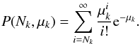 (A.1)Combining all multiplicities and the two datasets yields the test statistic λIC
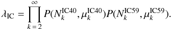 (A.2)In addition to the IceCube information (i.e. number of doublets and multiplets of higher order) we add information obtained by the optical observations. The probability to observe NSN or more optical SN counterparts based on the expected number μSN of accidentally observed SN in coincidence with an IceCube multiplet (given by Eq. (8)) is given by the sum of Poisson probabilities:
 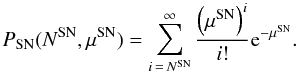 (A.3)If one or more optical counterparts were observed the significance could be improved by adding neutrino timing information as well as the distance information of the object found. The probability Pt to find a time difference of Δt or smaller between the first and the last neutrino event in the multiplet (defined by the maximal temporal difference of 100 s between the neutrino arrival times) due to a background fluctuation assuming a uniform background is given by
  (A.4)Hence, assuming a generic SN prediction of a 10 s wide neutrino pulse results in a factor of 10 lower chance probability.
Taking into account the SN distance allows us to compute the probability Pd to observe a background SN at a distance d < dSN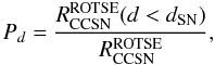 (A.5)where
  is the rate of SN observable by the ROTSE telescopes within a sphere of radius dSN
 is the total number of SN observable by ROTSE. Accidental coincidences will be distributed following the SN rate (i.e. the square of the distance) folded with ROTSE’s sensitivity as a function of distance εROTSE(d) (see Sect. 4). Signal events have a strong preference to close-by SNe, since only these will lead to a neutrino flux large enough to produce a detectable multiplet in IceCube. While ROTSE can only detect close-by SNe, more powerful telescopes can access a much larger volume and would essentially always detect a SN in their field of view. Hence, the additional factor Pd becomes important to account for the SN distance. The additional terms Pt and Pd for each observed SN light curve are combined with PSN yielding the test statistic λROTSE.
 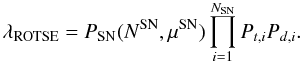 (A.6)Combining all information into one test statistic λ yields:
  (A.7)To obtain a proper confidence region for exclusion of the model we perform 10 000 Monte Carlo (MC) experiments for each combination of model parameters. The model prediction,
  and
and  , depends on the model parameters, Ejet, Γ and ρ. is obtained from the neutrino signal simulation weighted with the corresponding AB05 spectrum. The neutrino spectrum varies with Ejet and Γ as presented in Sect. 2. The number of predicted SNe, , depends on the number of neutrino multiplets, i.e. number of telescope pointings, folded with the sensitivity of the telescope. In our signal estimation we have not accounted for mixed multiplets due to a single SN neutrino in coincidence with a background neutrino. While in principle, these can be indentified through an optical counterpart, we estimate the rate to be at most a few percent of the pure, signal-only multiplets. We hence neglected the extra contribution. The average number of background multiplets
  is known from scrambling.
For each MC experiment the number of signal and background multiplets are drawn following a Poisson distribution. In case of the signal, the systematic uncertainties are included by smearing the Poisson mean, i.e. the Poisson mean is multiplied by a factor following a Gaussian distribution with mean one and a width given by the systematic uncertainties summarized in Sect. 5.
If an optical counterpart is drawn in the MC simulation ( ) we calculate the additional terms Pt and Pd following Eqs. (A.4) and (A.5). The time difference between the SN neutrinos is set to Δt = 10 s and the SN distance is thrown following a spatially isotropic distribution folded with ROTSE’s efficiency. For each MC experiment λ is calculated following Eq. (A.7). The fraction of MC experiments resulting in a smaller value of λ than that of the data sample (i.e. fraction of outcomes of the MC experiment which show worse agreement with the background-only hypothesis than the actual measurement) is the desired confidence level for the exclusion of this combination of model parameters.
All Tables
All Figures
|
Fig. 1 SN neutrino spectrum according to AB05 for one SN at distance 10 Mpc with the jet pointing to us. Different shades of gray indicate different Lorentz boost factors. Solid lines: Ejet = 3 × 1051 erg. Dotted line: Ejet = 0.3 × 1051 erg. Dashed line: Ejet = 30 × 1051 erg. |
| In the text | |
|
Fig. 2 The IceCube detector: The full detector consists of 86 strings with 60 DOMs attached to each string. Different colors/symbols indicate different deployment stages. The solid black line encircles the IC 59 configuration, while the dashed line indicates the smaller IC 40 configuration. |
| In the text | |
|
Fig. 3 Filter efficiency of Level 3 relative to Level 2 as function of energy for well-reconstructed events (IC 59). |
| In the text | |
|
Fig. 4 Expected number of SN neutrinos from a SN at distance 10 Mpc with a jet pointing towards Earth for different model parameter combinations (IC 59). |
| In the text | |
|
Fig. 5 Neutrino effective area at the final selection level for well-reconstructed events for IC 40 (blue squares) and IC 59 (red circles). |
| In the text | |
|
Fig. 6 Angular difference between the reconstructed directions of two neutrinos with identical true direction for jet parameters Γ = 3 and Ejet = 3 × 1051 erg (IC 59). |
| In the text | |
|
Fig. 7 Doublet resolution using an ordinary mean (blue circles), a weighted mean (red squares) compared to the singlet resolution (green triangles) for signal neutrinos (Γ = 3, Ejet = 3 × 1051 erg). Applying the directional coincidence cut ΔΨ < 4° (black triangles) keeps mainly well-reconstructed doublets and yields a further improvement of the doublet resolution (IC 59). |
| In the text | |
|
Fig. 8 Deviation of reconstructed multiplet direction from true direction (IC 59). The black box shows ROTSE’s field of view of 1.85° × 1.85°. |
| In the text | |
|
Fig. 9 Efficiency to find inserted SNe as a function of the apparent peak magnitude averaged over all alert directions assuming a template light curve. |
| In the text | |
|
Fig. 10 Black curve: efficiency to detect core-collapse SN as a function of the distance to the SN assuming an absolute R-band magnitude of − 18 ± 1. Shaded region: lower bound assuming an absolute magnitude of − 17, upper bound assuming − 19. The breaks in the shaded regions are connected to the binning in Fig. 9. The binning effect is washed out in the black curve due to the assumed uncertainty in the absolute magnitude distribution of ± 1. |
| In the text | |
|
Fig. 11 Systematic uncertainties (relative to the predicted SN neutrino event rate) depending on model parameters Γ and Ejet. |
| In the text | |
|
Fig. 12 Limits on the choked jet SN model Ando & Beacom (2005) for different Lorentz boost factors Γ as a function of the rate of SNe with jets ρ and the jet energy Ejet. The colored regions are excluded at 90% confidence level. Horizontal dashed lines indicate a fraction of SNe with jets of 100%, 10% or 1% (relative to an assumed CCSN rate of 1 per year within a sphere of radius 10 Mpc). |
| In the text | |
Current usage metrics show cumulative count of Article Views (full-text article views including HTML views, PDF and ePub downloads, according to the available data) and Abstracts Views on Vision4Press platform.
Data correspond to usage on the plateform after 2015. The current usage metrics is available 48-96 hours after online publication and is updated daily on week days.
Initial download of the metrics may take a while.