| Issue |
A&A
Volume 539, March 2012
|
|
|---|---|---|
| Article Number | A158 | |
| Number of page(s) | 5 | |
| Section | Planets and planetary systems | |
| DOI | https://doi.org/10.1051/0004-6361/201117767 | |
| Published online | 13 March 2012 | |
Nonextensive distributions of asteroid rotation periods and diameters
1 Programa de Engenharia Industrial, Escola Politécnica, Universidade Federal da Bahia, R. Aristides Novis 2, Federação, 40210-630 Salvador-BA, Brazil
e-mail: betzler.ssa@ftc.br
2 Instituto de Física and National Institute of Science and Technology for Complex Systems, Universidade Federal da Bahia, Campus Universitário de Ondina, 40210-340 Salvador-BA, Brazil
e-mail: ernesto@ufba.br
Received: 25 July 2011
Accepted: 5 December 2011
Context. We investigate the distribution of asteroid rotation periods from different regions of the solar system and diameter distributions of near-Earth asteroids (NEAs).
Aims. We aim to verify if nonextensive statistics satisfactorily describes the data.
Methods. Light curve data were taken from the Planetary Database System (PDS) with Rel ≥ 2. We also considered the taxonomic class and region of the solar system. Data of NEA were taken from the Minor Planet Center.
Results. The rotation periods of asteroids follow a q-Gaussian with q = 2.6 regardless of taxonomy, diameter, or region of the solar system of the object. The distribution of rotation periods is influenced by observational bias. The diameters of NEAs are described by a q-exponential with q = 1.3. According to this distribution, there are expected to be 994 ± 30 NEAs with diameters greater than 1 km.
Key words: minor planets, asteroids: general
© ESO, 2012
1. Introduction
Asteroids and comets are primordial bodies of the solar system (SS). The study of the physical properties of these objects may lead to a better understanding of the SS formation processes, and, by inference, of the hundreds of exo-solar systems already known. The distribution of rotation periods and diameters of asteroids are two parameters that may yield information concerning the evolution of the SS. The first attempt to describe histograms of asteroid rotation periods was made by Harris & Burns (1979). This work and others that have followed have shown that rotation periods of big asteroids (D > 30–40 km) follow a Maxwellian distribution. Harris & Pravec (2000) have analyzed a sample with 984 objects and have confirmed that the distribution of rotation periods of asteroids with diameters D ≥ 40 km is Maxwellian, with 99% confidence, though this hypothesis can be rejected at 95% confidence. They suggest that objects within this diameter range are primordial, or originated from collisions of primordial bodies. It is known that for medium sized (10 < D ≤ 40 km ) and small (D < 10 km) asteroids, the distribution of rotation periods is not Maxwellian. The analysis of the data suggests the existence of a spin-barrier for the asteroids with diameters between hundreds of meters and 10 km and with more than 11 rotations per day (d-1) (period of about 2.2 h). The absence of a substantial quantity of asteroids with periods of less than 2.2 h may be explained by the low degree of internal cohesion of these objects. The majority of the sample may contain rubble pile asteroids (Davis et al. 1979; Harris 1996) that are composed of fragments of rocks held together by self-gravitation. For objects below 0.2 km rotation periods shorter than the spin-barrier have been observed, suggesting that these objects have a high internal cohesion, which in turn implies that they may be monolithic bodies. The difficulty in modeling rotation periods of asteroids as a whole may be associated to the combined action of many mechanisms such as collisions (Paolicchi et al. 2002), gravitational interactions with planets (Scheeres et al. 2004), angular momentum exchange in binary or multiple asteroid systems (Scheeres 2002), or torques induced by solar radiation, known as the YORP effect (from Yarkovsky-O’Keefe-Radzievskii-Paddack; Rubincam 2000). The YORP effect strongly depends on the shape and size of the object and its distance to the Sun.
Near-Earth asteroids (NEAs) are a subgroup of SS asteroids, whose heliocentric orbits lead them close to the Earth’s orbit. More than 7000 NEAs are known up to 2011. The study of these objects is relevant because it may bring information regarding the birth and dynamic evolution of the SS. Moreover, these objects might collide with the Earth with obvious catastrophic consequences (Alvarez et al. 1980). They also may be sources of raw material for future space projects.
The evaluation of the number of asteroids per year that may reach the Earth as a function of their diameters is essential for determining the potential risk of a collision. One of the first attempts to estimate this flux was made by Shoemaker et al. (1979).
The impact flux may be taken from the accumulated distribution of NEA diameters. This distribution is indirectly obtained through current asteroid surveys, via the absolute magnitude H. The distribution of absolute magnitude H is described by Jedicke et al. (2002),  (1)where N is the number of objects, α is the “slope parameter” and β is a constant. This relation asymptotically models the observed distribution of H. Departure from this power law is probably associated with the observational bias caused by physical and dynamical properties of the asteroids (orbital elements, size, albedo), and instrumental limitations (CCD, detection software, among others). Accordingly, Eq. (1) may be used to describe a given population of asteroids if a correction of the bias is made in the raw data.
The asteroid diameter, D, may be given as a function of their absolute magnitudes and their albedos,  , according to Bowell et al. (1989),
  (2)The albedo is the rate of superficial reflection and its value is essential for estimating the asteroid diameters. The albedo values of asteroids vary according to the superficial mineralogical composition (taxonomic complex) and the object’s shape. Typical values range from 0.06 ± 0.02 for low-albedo objects of C taxonomic complex up to 0.46 ± 0.06 for high-albedo objects of V-type (Warner et al. 2009).
Combination of Eqs. (1) and (2) leads to a power law behavior:  (3)The parameters were estimated by Stuart (2003), b = 1.95 (α = b/5, admitting the same albedo for the entire sample) k = 1090, and D is given in km. According to this expression and taking into account the uncertainties of the measures, Stuart & Binzel (2004) have estimated that there may exist 1090 ± 180 objects with diameters equal to, or greater than, 1 km (H = 17.8).
2. Nonextensive statistics
In order to model the accumulated distribution of asteroid periods and diameters, we have applied results from the Tsallis nonextensive statistics. This choice comes from the observational evidence that astrophysical systems are somehow related to nonextensive behavior. It is known that systems with long-range interactions (typically gravitational systems) are not properly described by Boltzmann-Gibbs statistical mechanics (Landsberg 1990). During the past two decades the nonextensive statistical mechanics have been continuously developed, which is a generalization of the Boltzmann-Gibbs statistical mechanics. Tsallis proposed in 1988 (Tsallis 1988) a generalization of the entropy,  (4)where pi is the probability of the i-th microscopical state, W is the number of states, k is a constant (Boltzmann’s constant) and q is the entropic index. The Boltzmann-Gibbs entropy
  is recovered if q → 1. It was soon realized that the nonextensive statistical mechanics could be successfully applied to self-gravitating systems: Plastino & Plastino (1993) found a possible solution to the problem of a self-gravitating system with total mass, total energy, and total entropy simultaneously finite, within a nonextensive framework. Many examples of nonextensivity in astrophysical systems may be found. We list some instances. Nonextensivity was observed in the analysis of magnetic field at distant heliosphere associated to the solar wind observed by Voyager 1 and 2 (Burlaga & Viñas 2005; Burlaga & Ness 2009, 2010). The distribution of stellar rotational velocities in the Pleiades open cluster was found to be satisfactorily modeled by a q-Maxwellian distribution (Soares et al. 2006). The problem of Jeans gravitational instability was considered according to nonextensive kinetic theory (Lima et al. 2002). Nonextensive statistical mechanics was also used to describe galaxy clustering processes (Wuensche et al. 2004) and temperature fluctuation of the cosmic background radiation (Bernui et al. 2006, 2007). Fluxes of cosmic rays can be accurately described by distributions that emerge from nonextensive statistical mechanics (Tsallis et al. 2003). A list of more instances of applications of nonextensive statistical mechanics in astrophysical systems may be found in Tsallis (2009).
It is important to mention that the index q has a physical interpretation – it expresses the degree of nonextensivity – and for some systems it can be determined a priori (based on dynamical properties). Indeed, a nonextensive system is characterized by a q-triplet and not just by a single q (additional information can be found in Tsallis 2009). This triplet was already obtained in an astrophysical system (Burlaga & Vinhas 2005; Burlaga & Ness 2009, 2010).
Maximization of Sq under proper constraints leads to distributions that are generalizations of those that appear within the Boltzmann-Gibbs context. For instance, if it is required that the (generalized) energy of the system is constant (Curado & Tsallis 1991), the probability distribution that emerges is a q-exponential,  (5)βq is the Lagrange multiplier (not to confound with β of Eq. (1)). The q-exponential function is defined as (Tsallis 1994)
 ![\begin{equation} \exp_q x = [1 + (1-q) x]_+^{\frac{1}{1-q}}. \label{eq:qexp-definition} \end{equation}](/articles/aa/full_html/2012/03/aa17767-11/aa17767-11-eq36.png) (6)The symbol [a] + means that [a] = a if a > 0 and [a] = 0 if a ≤ 0. The q-exponential is a generalization of the exponential function, which is recovered if q → 1. If the constraint imposes that the (generalized) variance of the distribution is constant, then the distribution that maximizes Sq is a q-Gaussian (Tsallis et al. 1995; Prato & Tsallis 1999),
(6)The symbol [a] + means that [a] = a if a > 0 and [a] = 0 if a ≤ 0. The q-exponential is a generalization of the exponential function, which is recovered if q → 1. If the constraint imposes that the (generalized) variance of the distribution is constant, then the distribution that maximizes Sq is a q-Gaussian (Tsallis et al. 1995; Prato & Tsallis 1999),  (7)The q-Gaussian recovers the usual Gaussian at q = 1, and particular values of the entropic index q turn p(x) into various known distributions, such as the Lorentz distribution, uniform distribution, Dirac’s delta (see Tsallis et al. 1995; and Prato & Tsallis 1999, for details).
The Lagrange parameter βq also has a precise physical meaning. Within the statistical mechanics context, the Lagrange parameter βq in Eq. (5) is related to the inverse of the temperature (β1 = 1/(kT) if q = 1), and in Eq. (7) it is related to the inverse of the variance (β1 = 1/(2σ2) in normal diffusion, σ2 is the variance). Generally speaking, the inverse of the Lagrange parameters are associated to the finiteness of the first or second moments of the distribution.
Inverse cumulative distributions of the family of the q-exponentials are usually, and conveniently, graphically represented by means of log -log plots, and Fig. 1 shows a general instance for the function N ≥ (x) = Mexpq( − βqxγ). γ is a general parameter that recovers the q-exponential (γ = 1), the q-Gaussian (γ = 2), and in a generalized scheme, it may assume other values, i.e. it may represent other distributions. The tails of q-exponentials are power laws (expq( − βqx) ~ [(q − 1)βqx] 1/(1 − q) for x ≫ 1 and q > 1) and therefore the slope of the asymptotical power law regime in a log-log plot leads to the determination of the parameter q (slope = γ/(1 − q) for general γ not necessarily equal to one). For low values of the independent variable x (we are assuming x > 0) this graphical representation displays a region that appears to be quasi-flat in this log -log plot; of course it is not flat, once the function is monotonically decreasing by construction. We call this region “quasi-flat” to distinguish it from the asymptotical power law region. Figure 1 shows the intersection of two straight lines that represent the two regimes. The intersection is the transition point between the regimes (the crossover), and it is given by ![\begin{equation} x^*=\frac{1}{\left[(q-1)\beta_q\right]^{\frac{1}{\gamma}}}\cdot \label{eq:crossover} \end{equation}](/articles/aa/full_html/2012/03/aa17767-11/aa17767-11-eq60.png) (8)Figure 1 also displays an ordinary (q = 1) exponential, for comparison. Exponentials of negative arguments decay vary fast, and when represented in log -log plots this feature becomes clear, once the exponential asymptotically presents slope → −∞. Coherently Eq. (8) gives x∗ → ∞ for q = 1, indicating that there is no crossover of an exponential to a power law regime.
(8)Figure 1 also displays an ordinary (q = 1) exponential, for comparison. Exponentials of negative arguments decay vary fast, and when represented in log -log plots this feature becomes clear, once the exponential asymptotically presents slope → −∞. Coherently Eq. (8) gives x∗ → ∞ for q = 1, indicating that there is no crossover of an exponential to a power law regime.
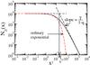 |
Fig. 1 Inverse cumulative distribution of a generalized q-exponential, N ≥ (x) = Mexpq( − βqxγ). γ = 1 is a q-exponential, γ = 2 is a q-Gaussian, M is the size of the sample. Values of the parameters for this particular instance are q = 1.5, βq = 0.1 and M = 104. The transition point (x ∗ )γ given by Eq. (8) is indicated. Dashed curve (red online) is an ordinary (q = 1) exponential with β1 = 0.1 and M = 104. Evidently, the tail behavior is entirely different from both curves. |
We have found that the distribution of diameters of NEAs follows a q-exponential and the observed rotation periods of all asteroids, regardless of their diameters, mineralogical composition, or region of the SS, are well approximated by a q-Gaussian. We investigated two samples from databases of different years to verify the effect of the observational bias.
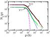 |
Fig. 2 Decreasing cumulative distribution of periods of V7 (green dots on line) and V11 (black dots online) of PDS (NASA) with Rel ≥ 2, and superposed q-Gaussians (N ≥ (p) = Mexpq( − βqp2)). V7: q = 2.0, βq = 0.0161 h-2, M = 1621; V11: q = 2.6, βq = 0.025 h-2, M = 3567. Fittings of the periods of V7 for P > 50 h are poor. This does not happen with V11, and it possibly indicates a better accuracy of the data. Dashed (violet online) and dot-dashed (magenta online) lines are normal (q = 1) Gaussians, with β1 = 0.0161 h-2, M = 1621, and β1 = 0.025 h-2, M = 3567. |
3. Observational data
One important problem in the evaluation of distributions of rotation periods and diameters of asteroids (and of course the same applies for other observables) is that the data are possibly influenced by observational bias. In order to take this effect into account, we considered samples from databases of two different years: 2005 and 2010 for rotation periods, and 2001 and 2010 for asteroid diameters.
Two versions of the lightcurve derived data, available at the Planetary Database System (PDS), were used: version 7 (V7), with 1971 periods, and version 11 (V11), with 4310 periods (Harris et al. 2005, 2010). The periods are classified according to a quality code of the reliability of the estimated period, defined by Harris & Young (1983). We used periods with Rel ≥ 2 (Rel for reliability) that means they are accurate to ≈ 20%, which resulted in 1621 entries for the V7 and 3567 asteroids for the V11. Cross-checking the V11 sample with a compilation of taxonomic classifications, also available at PDS, revealed that about 40% (1487) of these asteroids have approximately known mineralogical composition. The asteroids were separated into three main classes: C , S, and X complexes, following the SMASS II system of Bus & Binzel (2002), with 503, 663, and 321 objects, respectively. The diameters of these subsamples were calculated with Eq. (2) with the absolute magnitude H available from MPCORB – Minor Planet Center Orbit Database (MPC 2010).
We also used two versions of the compilation of absolute magnitudes H, namely that of Oct., 2001, with 1649 NEAs (similar to Stuart’s 2001, procedure) and Oct., 2010, with 7078 objects (MPC 2010). We adopted pV = 0.14 ± 0.02 for the NEAs population albedo. This value was estimated by Stuart & Binzel (2004) and it takes into account the great variety of taxonomic types that are found in the NEAs (Binzel et al. 2004). In order to estimate the validity of the diameters estimated by Eq. (2), we considered the diameters of 101 asteroids obtained from Spitzer Space Telescope data (Trilling et al. 2010). This resulted in an error of about 20%. We considered that this value, though not small, is reasonable for the purposes of our study.
4. Distribution of rotation periods
Figure 2 shows the decreasing cumulative distribution of periods of V7 and V11, and superposed q-Gaussians (N ≥ (p) = Mexpq(−βqp2)) and obviously, these functions quite satisfactorily describe almost all data with q = 2.0 ± 0.1, βq = 0.016 ± 0.001 h-2 and M = 1621 (M is the number of objects) for V7, and q = 2.6 ± 0.2, βq = 0.025 ± 0.002 h-2 and M = 3567 for V11. Parameters were found by a nonlinear leasts squares method. Figure 2 also presents two ordinary Gaussians, and evidently, these q = 1 distributions are completely unable to represent the data. The confidence level for both fits is 95%, according to an χ2 test. This suggests that the distribution does not depend on (i) the diameters, (ii) the mineralogical composition, or (iii) the region of the SS in which the object is found. The latter is particularly important once the sample includes NEAs, trans-Neptunian objects (TNO), asteroids from the main belt (MBA), Jupiter trojans (JT) and dwarf planets such as Ceres and Pluto. The values of the entropic indexes (q = 2.0 for V7 and q = 2.6 for V11) – rather distant from unity, that is, distant from the Maxwellian distribution – may indicate that long-range interactions play an essential role in the distribution of rotation periods. According to Eq. (8) (with x∗ ≡ p∗, γ = 2), the transition point is p∗ = 7.91 ± 0.01 h (f ~ 3 d-1) for the data of V7, and p∗ = 5.00 ± 0.02 h (f ~ 5 d-1) for the data of V11. The transition points for both samples differ from the critical period of the spin barrier, and therefore the transition is not a consequence of physical processes. Warner & Harris (2010) have demonstrated that the periods are more accurately determined for objects with periods p ≤ 8 h and light curve amplitudes A ≥ 0.3 mag, so we conclude that the difference between the transition points of the two versions is caused by observational bias.
We separately considered the taxonomic complexes C, S, and X (V11), shown in Fig. 3, and found that all of them are properly described by q-Gaussians within 95% of confidence level (q = 2.6 ± 0.2 and βq = 0.021 ± 0.002 h-2 for S, q = 2.0 ± 0.1 and βq = 0.015 ± 0.001 h-2 for C and q = 2.0 ± 0.1 and βq = 0.010 ± 0.007 h-2 for X; fitted curves are not indicated in Fig. 3). The difference between the parameters for each complex is related to the size of the sample, and they are statistically similar. The fittings for the C and X complexes can be improved if we admit that the number of objects are 10% higher than that found in the sample. The transition point p∗ decreases from V7 to V11, and this may be an indication that the fraction of fast rotators (f ≥ 5 d-1) may still be underestimated.
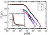 |
Fig. 3 Log-log plot of the decreasing cumulative distribution of periods of 3567 asteroids (dots) with Rel ≥ 2 taken from the PDS (NASA) and a q-Gaussian distribution (N ≥ (p) = Mexpq(−βqp2)) (solid line), with q = 2.6, βq = 0.025 h-2, M = 3567. The other curves are 663 S-complex asteroids (diamonds, blue online), 503 C-complex asteroids (squares, green online), 321 X-complex asteroids (triangles, magenta online). Inset shows the 3567 asteroids and the q-Gaussian in a linear-linear plot. |
5. Distribution of near-Earth asteroid diameters
We have found that the decreasing cumulative distribution of diameters of NEAs can be fitted by q-exponentials. The fitting of a q-exponential to the diameters of 7078 NEAs (N ≥ (D) = Mexpq(−βqD)), shown in Fig. 4, is quite good for the entire range of the data, with a confidence level of 95%: q = 1.3 ± 0.1 and βq = 3.0 ± 0.2 km-1 (found with the nonlinear leasts squares method). This distribution, however, is influenced by observational bias. The q-exponential distribution can be used to determine the point at which the sample is supposed to be complete. Figure 4 compares q-exponentials that fit the observed diameter distribution of known NEAs in October 2001 and October 2010. The observed diameter distribution of the 2001 database follows a q-exponential with q = 1.3 ± 0.1 and βq = 1.5 ± 0.1 km-1 and the same confidence level. The figure also shows normal (q = 1) exponentials, and their inadequacy can be promptly verified in the representation of the whole data range.
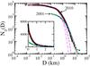 |
Fig. 4 Decreasing cumulative distribution of diameters of known NEAs in 2001 (1649 objects, green dots) and in 2010 (7078 objects, black dots). Solid lines are best fits of q-exponentials (N ≥ (D) = Mexpq(−βqD)). Blue line (2001): q = 1.3, βq = 1.5 km-1, M = 1649, red line (2010): q = 1.3, βq = 3 km-1, M = 7078. Normal exponentials (q = 1) are displayed in the main panel for comparison (dashed violet, with β1 = 1.5 km-1, M = 1649, and dot-dashed magenta, with β1 = 3 km-1, M = 7078). |
Once the value of q is the same for the 2001 and 2010 samples, we may argue that this parameter is not influenced by the bias in this case, and it reflects real physical processes. Both curves are practically identical in the power-law region, and the point of transition to the quasi-flat region differs, as expressed by the different values of βq. The value of q = 1.3 (different from one) is an indication that not only collisional processes are involved in forming these objects. Other mechanisms may also be present: the YORP effect may lead to the decrease of the rotation period up to the point of rupture. This fragmentation process may yield the formation of binary or multiple systems. About (15 ± 4)% of NEAs with D ≥ 0.3 km and rotation periods between 2 and 3 h possibly are binary systems (Pravec et al. 2007). The transition points according to Eq. (8) (with x∗ ≡ D∗, γ = 1) are D∗ = 2.22 ± 0.05 km (2001), and D∗ = 1.11 ± 0.05 km (2010).
The sample is complete up to the upper limit of these intervals, 2.22 + 0.05 = 2.27 km (H = 16) for 2001 basis and 1.11 + 0.05 = 1.16 km (H = 17.5) for 2010 basis. The number of NEA with D ≥ 2.27 km is virtually the same for the sample of 2001 and 2010 (166 ± 8 objects). This is confirmation of the sample completeness up to H ~ 15 (Jedicke et al. 2002), and the extension of this limit up to H ~ 16 (Harris 2008). Once there has been an increase in the efficiency of detection and in the number of surveys (Stokes et al. 2002; Larson 2007), we conclude that the parameter βq indicates the limit of sample completeness. For D ≥ 1.16 km, the 2010 data are best described by a power-law. We found for Eq. (3), k = 994 ± 30 and b = 2.24 ± 0.01, with correlation coefficient R2 = 0.987. The value of b corresponds to α = 0.448 ± 0.002 in Eq. (1), which is a reasonable value compared to the slope of 0.44 found by Zavodny et al. (2008). The value of q may be found from b using q = 1 + 1/b, thus q = 1.446 ± 0.001, which is within the interval found in the whole sample. According to the distribution we found 994 ± 30 asteroids with D ≥ 1 km (H ≤ 17.7), in a close agreement with Mainzer et al. (2011). Distribution analyses of the MBA and TNO diameters according to lines similar to those used in this work are welcome.
Acknowledgments
This work was partially supported by FAPESB, through the program PRONEX (Brazilian funding agency). We are grateful to J. S. Stuart for important remarks and suggestions.
References
- Alvarez, L. W., Alvarez, W., Asaro, F., & Michel, H. V. 1980, Science, 208, 1095 [NASA ADS] [CrossRef] [Google Scholar]
- Bernui, A., Tsallis, C., & Villela, T. 2006, Phys. Lett. A, 356, 426 [NASA ADS] [CrossRef] [Google Scholar]
- Bernui, A., Tsallis, C., & Villela, T. 2007, Europhys. Lett., 78, 19001 [NASA ADS] [CrossRef] [EDP Sciences] [Google Scholar]
- Binzel, R. P., Rivkin, A. S., Stuart, J. S., et al. 2004, Icarus, 170, 259 [NASA ADS] [CrossRef] [Google Scholar]
- Bowell, E., Hapke, B., Domingue, D., et al. 1989, in Asteroids II, ed. R. P. Binzel, T. Gehrels, & M. S. Matthews (Tucson: Univ. Arizona Press), 524 [Google Scholar]
- Burlaga, L. F., & Viñas, A. F. 2005, Physica A, 356, 375 [NASA ADS] [CrossRef] [Google Scholar]
- Burlaga, L. F., & Ness, N. F. 2009, ApJ, 703, 311 [NASA ADS] [CrossRef] [Google Scholar]
- Burlaga, L. F., & Ness, N. F. 2010, ApJ, 725, 1306 [NASA ADS] [CrossRef] [Google Scholar]
- Bus, S. J., & Binzel, R. P. 2002, Icarus, 158, 146 [NASA ADS] [CrossRef] [Google Scholar]
- Curado, E. M. F., & Tsallis, C. 1991, J. Phys. A, 24, L69; Corrigenda: 1991, 24, 3187 and 1992, 25, 1019 [NASA ADS] [CrossRef] [Google Scholar]
- Davis, D. R., Chapman, C. R., Greenberg, R., Weidenschilling, S. J., & Harris, A. W. 1979, in Asteroids, ed. T. Gehrels (Tucson: Univ. Arizona Press), 528 [Google Scholar]
- Harris, A. W. 1996, in Lunar and Planetary Institute Conference Abstracts, 27, 493 [Google Scholar]
- Harris, A. W. 2008, Nature, 453, 1178 [NASA ADS] [CrossRef] [Google Scholar]
- Harris, A. W., & Burns, J. A. 1979, Icarus, 40, 115 [NASA ADS] [CrossRef] [Google Scholar]
- Harris, A. W., & Young, J. W. 1983, Icarus, 54, 59 [NASA ADS] [CrossRef] [Google Scholar]
- Harris, A. W., Warner, B. D., & Pravec, P. 2005, Asteroid Lightcurve Derived Data V7.0, EAR-A-5-DDR-DERIVED-LIGHTCURVE-V7.0, NASA Planetary Data System [Google Scholar]
- Harris, A. W., Warner, B. D., & Pravec, P. 2010, Asteroid Lightcurve Derived Data V11.0, EAR-A-5-DDR-DERIVED-LIGHTCURVE-V11.0, NASA Planetary Data System [Google Scholar]
- Jedicke, R., Larsen, J., & Spahr, T. 2002, in Asteroids III, ed. W. F. Bottke Jr., A. Cellino, P. Paolicchi, & R. P. Binzel (Tucson: Univ. of Arizona Press), 71 [Google Scholar]
- Landsberg, P. T. 1990, Thermodynamics and Statistical Mechanics (New York: Dover) [Google Scholar]
- Larson, S. 2007, in Near Earth Objects, our Celestial Neighbors: Opportunity and Risk, ed. G. B. Valsecchi, D. Vokrouhlicky, & A. Milani (Cambridge: Cambridge University Press), Proc. IAU Symp., 236, 323 [Google Scholar]
- Lima, J. A. S., Silva, R., & Santos, J. 2002, A&A, 396, 309 [NASA ADS] [CrossRef] [EDP Sciences] [Google Scholar]
- Mainzer, A., Grav, T., Bauer, J., et al. 2011, ApJ, 743, 156 [NASA ADS] [CrossRef] [Google Scholar]
- Minor Planet Center 2010, MPCORB, http://www.minorplanetcenter.org/iau/MPCORB.html [Google Scholar]
- Paolicchi, P., Burns, J. A., & Weidenschilling, S. J. 2002, in Asteroids III, ed. W. F. Bottke, A. Cellino, P. Paolicchi, & R. P. Binzel (Tucson: Univ. Arizona Press), 517 [Google Scholar]
- Plastino, A. R., & Plastino, A. 1993, Phys. Lett. A, 174, 384 [NASA ADS] [CrossRef] [MathSciNet] [Google Scholar]
- Prato, D., & Tsallis, C. 1999, Phys. Rev. E, 60, 2398 [NASA ADS] [CrossRef] [Google Scholar]
- Pravec, P., & Harris, A. W. 2000, Icarus, 148, 12 [NASA ADS] [CrossRef] [Google Scholar]
- Pravec, P., Harris, A. W., & Warner, B. D. 2007, in Near Earth Objects, our Celestial Neighbors: Opportunity and Risk, ed. G. B. Valsecchi, D. Vokrouhlicky, & A. Milani (Cambridge: Cambridge University Press), Proc. IAU Symp., 236, 167 [Google Scholar]
- Rubincam, D. P. 2000, Icarus, 148, 2 [NASA ADS] [CrossRef] [Google Scholar]
- Scheeres, D. J. 2002, Icarus, 159, 271 [NASA ADS] [CrossRef] [Google Scholar]
- Scheeres, D. J., Marzari, F., & Rossi, A. 2004, Icarus, 170, 312 [NASA ADS] [CrossRef] [Google Scholar]
- Shoemaker, E. M., Williams, J. G., Helin, E. F., & Wolfe, R. F. 1979, in Asteroids, ed. T. Gehrels (Tucson: Univ. Arizona Press), 253 [Google Scholar]
- Soares, B. B., Carvalho, J. C., do Nascimento, J. D., Jr., & de Medeiros, J. R. 2006, Physica A, 364, 413 [NASA ADS] [CrossRef] [MathSciNet] [Google Scholar]
- Stokes, G. H., Evans, J. B., & Larson, S. M. 2002, in Asteroids III, ed. W. F. Bottke Jr., A. Cellino, P. Paolicchi, & R. P. Binzel (Tucson: Univ. of Arizona Press), 45 [Google Scholar]
- Stuart, J. C. 2001, Science, 294, 1691 [NASA ADS] [CrossRef] [Google Scholar]
- Stuart, J. S. 2003, Ph.D. Thesis, MIT [Google Scholar]
- Stuart, J. S., & Binzel, R. P. 2004, Icarus, 170, 295 [NASA ADS] [CrossRef] [Google Scholar]
- Trilling, D. E., Mueller, M., Hora, J. L., et al. 2010, ApJ, 140, 770 [Google Scholar]
- Tsallis, C. 1988, J. Stat. Phys., 52, 479 [NASA ADS] [CrossRef] [MathSciNet] [Google Scholar]
- Tsallis, C. 1994, Quimica Nova, 17, 468 [Google Scholar]
- Tsallis, C. 2009, Introduction to Nonextensive Statistical Mechanics – Approaching a Complex World (New York: Springer) [Google Scholar]
- Tsallis, C., Levy, S. V. F., de Souza, A. M. C., & Maynard, R. 1995, Phys. Rev. Lett., 75, 3589; erratum: 1996, 77, 5442 [NASA ADS] [CrossRef] [MathSciNet] [PubMed] [Google Scholar]
- Tsallis, C., Anjos, J. C., & Borges, E. P. 2003, Phys. Lett. A, 310, 372 [NASA ADS] [CrossRef] [Google Scholar]
- Warner, B. D., & Harris, A. W. 2010, BAAS, 42, 1051 [NASA ADS] [Google Scholar]
- Warner, B. D., Harris, A. W., & Pravec, P. 2009, Icarus, 202, 134 [NASA ADS] [CrossRef] [Google Scholar]
- Wuensche, C. A., Ribeiro, A. L. B., Ramos, F. M., & Rosa, R. R. 2004, Physica A, 344, 743 [NASA ADS] [CrossRef] [Google Scholar]
- Zavodny, M., Jedicke, R., Beshore, E. C., Bernardi, F., & Larson, S. 2008, Icarus, 198, 284 [NASA ADS] [CrossRef] [Google Scholar]
All Figures
|
Fig. 1 Inverse cumulative distribution of a generalized q-exponential, N ≥ (x) = Mexpq( − βqxγ). γ = 1 is a q-exponential, γ = 2 is a q-Gaussian, M is the size of the sample. Values of the parameters for this particular instance are q = 1.5, βq = 0.1 and M = 104. The transition point (x ∗ )γ given by Eq. (8) is indicated. Dashed curve (red online) is an ordinary (q = 1) exponential with β1 = 0.1 and M = 104. Evidently, the tail behavior is entirely different from both curves. |
| In the text | |
|
Fig. 2 Decreasing cumulative distribution of periods of V7 (green dots on line) and V11 (black dots online) of PDS (NASA) with Rel ≥ 2, and superposed q-Gaussians (N ≥ (p) = Mexpq( − βqp2)). V7: q = 2.0, βq = 0.0161 h-2, M = 1621; V11: q = 2.6, βq = 0.025 h-2, M = 3567. Fittings of the periods of V7 for P > 50 h are poor. This does not happen with V11, and it possibly indicates a better accuracy of the data. Dashed (violet online) and dot-dashed (magenta online) lines are normal (q = 1) Gaussians, with β1 = 0.0161 h-2, M = 1621, and β1 = 0.025 h-2, M = 3567. |
| In the text | |
|
Fig. 3 Log-log plot of the decreasing cumulative distribution of periods of 3567 asteroids (dots) with Rel ≥ 2 taken from the PDS (NASA) and a q-Gaussian distribution (N ≥ (p) = Mexpq(−βqp2)) (solid line), with q = 2.6, βq = 0.025 h-2, M = 3567. The other curves are 663 S-complex asteroids (diamonds, blue online), 503 C-complex asteroids (squares, green online), 321 X-complex asteroids (triangles, magenta online). Inset shows the 3567 asteroids and the q-Gaussian in a linear-linear plot. |
| In the text | |
|
Fig. 4 Decreasing cumulative distribution of diameters of known NEAs in 2001 (1649 objects, green dots) and in 2010 (7078 objects, black dots). Solid lines are best fits of q-exponentials (N ≥ (D) = Mexpq(−βqD)). Blue line (2001): q = 1.3, βq = 1.5 km-1, M = 1649, red line (2010): q = 1.3, βq = 3 km-1, M = 7078. Normal exponentials (q = 1) are displayed in the main panel for comparison (dashed violet, with β1 = 1.5 km-1, M = 1649, and dot-dashed magenta, with β1 = 3 km-1, M = 7078). |
| In the text | |
Current usage metrics show cumulative count of Article Views (full-text article views including HTML views, PDF and ePub downloads, according to the available data) and Abstracts Views on Vision4Press platform.
Data correspond to usage on the plateform after 2015. The current usage metrics is available 48-96 hours after online publication and is updated daily on week days.
Initial download of the metrics may take a while.