| Issue |
A&A
Volume 539, March 2012
|
|
|---|---|---|
| Article Number | A140 | |
| Number of page(s) | 11 | |
| Section | Planets and planetary systems | |
| DOI | https://doi.org/10.1051/0004-6361/201117102 | |
| Published online | 07 March 2012 | |
Multiwavelength flux variations induced by stellar magnetic activity: effects on planetary transits
1 Dipartimento di Fisica ed Astronomia, Università di Catania, via Santa Sofia 78, 95123 Catania, Italy
e-mail: This email address is being protected from spambots. You need JavaScript enabled to view it.
2 INAF – Osservatorio Astronomico di Palermo, Piazza del Parlamento 1, 90134 Palermo, Italy
3 INAF – Osservatorio Astrofisico di Catania, via Santa Sofia 78, 95123 Catania, Italy
e-mail: This email address is being protected from spambots. You need JavaScript enabled to view it.
Received: 18 April 2011
Accepted: 16 January 2012
Abstract
Stellar magnetic activity is a source of noise in the study of the transits of extrasolar planets. It induces flux variations that significantly affect the transit depth determination and the derivations of planetary and stellar parameters. Furthermore, the colour dependence of stellar activity may significantly influence the characterization of planetary atmospheres. Here we present a systematic approach to quantify the corresponding stellar flux variations as a function of wavelength bands. We consider a star with spots covering a given fraction of its disc and model the variability in both the UBVRIJHK photometric system and the Spitzer/IRAC wavebands for dwarf stars from G to M spectral types. We compare activity-induced flux variations in different passbands with planetary transits and quantify how they affect the determination of the planetary radius and the analysis of the transmission spectroscopy in the study of planetary atmospheres. We suggest that the monitoring of the systems by using broad-band photometry, from visible to infrared, helps us to constrain activity effects. The ratio of the relative variations in the stellar fluxes at short wavelength optical bands (e.g., U or B) to near-infrared ones (e.g., J or K) can be used to distinguish starspot brightness dips from planetary transits in a stellar light curve. In addition to the perturbations in the measurement of the planetary radius, we find that starspots can affect the determinations of both the relative semimajor axis and the inclination of the planetary orbit, which have a significant impact on the derivation of the stellar density from the transit light curves.
Key words: infrared: stars / techniques: photometric / stars: activity / stars: solar-type / starspots / planetary systems
© ESO, 2012
1. Introduction
The microvariability of active stars can hamper the measure of planetary transits and this can be a problem for targets with a solar-type or slightly higher magnetic activity level, i.e. main-sequence stars from late F to late G-type, or even worse for dM stars. The transit of a large group of spots on the solar surface causes a relative decrease in the optical flux of ~3.3 × 10⁻³ (Fröhlich & Lean 2004) and even in the absence of sunspots, the solar flux exhibits a modulation caused by bright structures, such as photospheric faculae. For comparison, the transit of a planet across the solar disc would produce a relative flux variation of the order of 10-4 and 10-2 for Earth and Jupiter, respectively. Therefore, the search for planetary transits in the presence of stellar activity requires techniques to filter out or fit the microvariability of the star. They are based on the observations of the flux variations outside transits along time intervals of at least two or three stellar rotations (cf., e.g., Aigrain & Irwin 2004; Moutou et al. 2005; Bonomo & Lanza 2008; Bonomo et al. 2009).
The detection of a transiting exoplanet is most likely at infrared wavelengths, where activity variations are smaller, especially when surveying dM-type stars. Moreover, their smaller size provides a more advantageous ratio of the planet to the host star radii, implying a greater transit depth for a given planetary radius, and suggests that for dM stars it could be easy to detect low mass planets (Butler et al. 2004; Nutzman & Charbonneau 2008; Deming et al. 2009). However, a large fraction of dM stars show a significant level of magnetic activity, which may be a crucial problem for the detection of transiting planets.
In the infrared bands, the ratio of the planet to the star emission increases remarkably, thus we can directly detect the radiation coming from the planet, allowing us to characterize the atmosphere during the occultation phase, i.e. through the analysis of the reflected planetary spectrum (emission spectroscopy, see Charbonneau et al. 1999; Cameron et al. 1999) or during the planetary transit in front of the star, i.e. by analysing the transmission spectrum of the planetary atmosphere (transmission spectroscopy, see Seager & Sasselov 2000; Brown 2001; Hubbard et al. 2001; Charbonneau et al. 2002). The analysis of infrared spectra has become a well-established field of transmission spectroscopy, since the infrared domain includes the most important spectral signatures of the main atmospheric moleculae, even if their detection is still controversial (Tinetti et al. 2007a; Swain et al. 2008; Désert et al. 2009; Sing et al. 2009; Agol et al. 2010; Désert et al. 2011a; Pallé et al. 2011; Gibson et al. 2011).
The observation of stars hosting planets in the optical and near-infrared wavebands is the main scientific objective of a number of ground-based projects (e.g. MEarth, see Nutzman & Charbonneau 2008). It is part of the program of the JWST (James Webb Space Telescope, Gardner et al. 2006) and will be the focus of the proposed ESA mission, EChO1 (Exoplanet Characterization Observatory, Tessenyi 2010), a space-borne telescope that will observe the visible-infrared spectra (0.4–16 μm) to characterize the physical properties of exoplanet atmospheres, searching for molecular spectral features and bio-markers. A significant part of the mission will be devoted to the observation of the atmospheres of super-Earth planets orbiting M dwarf stars for the aforementioned reasons.
A most widely used approach to constraining the properties of planetary atmospheres is that of measuring the transit depth in different passbands observed simultaneously. The selective absorption of the stellar radiation by the molecular species, present in the planetary atmosphere, may produce a variation in the apparent radius of the planet versus the central wavelength of the passband and can be used to detect them (e.g., Désert et al. 2011a,b; Croll et al. 2011). The presence of stellar magnetic variability, caused by cool spots, bright faculae, or magnetic surface inhomogeneities in general, can modify the transit depth and have a significant impact on the derivation of the dependence of the planetary radius on the wavelength (Pont et al. 2008; Czesla et al. 2009; Sing et al. 2009; Agol et al. 2010; Berta et al. 2011; Sing et al. 2011a,b; Désert et al. 2011a). We need to understand whether the apparent radius variations are due to molecular species in the planetary atmospheres or to stellar activity, whose effect is also expected to depend on the bandpass. In this respect, the quantification of activity-induced variations, as functions of wavelength, may be crucial requirement of the transmission spectroscopy to help in the characterization of the planet atmosphere and composition. The effects of activity are crucial above all for active sources, such as HD 189733, but the issue rises even for less active sources, such as GJ 1214.
Since the discovery of its planetary companion (Bouchy et al. 2005), HD 189733 has been the subject of intense observations in both the optical bands (Bakos et al. 2006; Winn et al. 2007; Pont et al. 2007, 2008; Sing et al. 2011b) and the infrared wavebands (Beaulieu et al. 2008; Sing et al. 2009; Désert et al. 2011a). It is a K-type star with strong chromospheric activity (Wright et al. 2004), which produces a quasi-periodic optical flux variation of ~1.3% (Winn et al. 2007) due to the rotation of a spotted stellar surface. The first accurate determination of the planetary system parameters was carried out by Bakos et al. (2006) through BVRI photometry; neglecting the effects of stellar variability, their planet-to-star radius ratio (0.156 ± 0.004) was found to be smaller than that of Bouchy et al. 2005 (0.172 ± 0.003)2. Winn et al. (2007) obtained radius measurements compatible with those of Bakos et al. (2006), again neglecting the effects of stellar variability. Even Pont et al. (2007) obtained results compatible with those of Bakos et al. (2006), in this case correcting their HST/ACS observations for the stellar variability; moreover, these authors expected that the starspots effect be reduced in the infrared because of a lower spot contrast. Through HST/NICMOS transit observations, correcting for the unocculted starspots, Sing et al. (2009) found a planet-to-star radius ratio of 0.15464 ± 0.00051 and 0.15496 ± 0.00028 at 1.66 and 1.87 μm, respectively, in agreement with the planet-to-star radius ratio of Bakos et al. (2006). In a multiwavelength set of HST/STIS optical transit light curves, Sing et al. (2011b) observed the typical signature of an occulted spot and, considering the effects of unocculted spots, estimated a spot correction to the transmitted spectrum of about 0.00292 ± 0.00113 as a fraction of the transit depth in the 320–375 nm passband, which is greater than in the 575–625 nm passband where it is negligible. Moreover, they clearly demonstrated the dependence of the planet-to-star radius ratio on the out-of-transit stellar flux showing that the transit is deeper when the star is fainter as expected as a consequence of unocculted spots present on the disc of the star during the transit (see Sect. 2.2). In Spitzer/IRAC wavebands, both Beaulieu et al. (2008) and Désert et al. (2011a) detected variations in the planet-to-star radius ratio. The former authors found that the infrared transit depth is smaller than in the optical (cf. Fig. 4 of Beaulieu et al. 2008) and the effect of stellar spots is to increase this depth. By correcting for this effect, they found that the transit depth is shallower by about 0.19%, at 3.6 μm, and 0.18%, at 5.8 μm. In the Spitzer/IRAC’s 3.6 μm band, the latter authors observed a greater Rp/R⋆ ratio in low brightness periods because of the presence of starspots, implying that the apparent planet-to-star radius ratio varies with stellar brightness from 0.15566 to 0.1545 ± 0.0003 (Désert et al. 2009) from low to high brightness periods, respectively.
An example of a less active M-type star that displays a rotational flux modulation of ~2% with a period of ~50 days is GJ 1214 (Charbonneau et al. 2009). Considering the error bars, the planet-to star radius ratio measurements through optical and near-infrared observations (Sada et al. 2010; Berta et al. 2011; Carter et al. 2011) are all consistent with the results of Charbonneau et al. 2009 (0.1162 ± 0.00067) obtained in the optical bands. Furthermore, Berta et al. (2011) detected variations in the planet-to-star radius ratio at different epochs and assessed the expected variation in this ratio due to stellar variability at optical wavelengths (see their Fig. 8). They stated that this effect may be neglected in Spitzer/IRAC bands. Croll et al. (2011) observed a deeper transit in the KS band than in the J band and, after taking into account the effects of the starspots, attributed this to a source of absorption in the 2.2–2.4 μm range, possibly associated with methane (Miller-Ricci & Fortney 2010).
A remarkable study of the starspot effects on the exoplanet sizes was carried out by Czesla et al. (2009) on the active star CoRoT-2 (Lanza et al. 2009; Huber et al. 2010). They pointed out the importance of the normalization of the transit profile to a common reference level to make different transits comparable with each other and show that the relative light loss during a transit is correlated significantly with the out-of-transit flux. The correlation is compatible with a distribution of starspots occulted during the transit that has a larger covering factor when the star is more active, i.e., when the out-of-transit flux is lower. A method for deriving the unperturbed transit profile is proposed by extrapolating the observed profiles towards their lower flux limit. A best fit to this profile gives a planet radius about 3% larger than that of Alonso et al. (2008), which is estimated without considering stellar activity in the CoRoT white bandpass (350–1100 nm).
The above examples illustrate how stellar magnetic activity has a significant impact on the transit depth and in the consequent derivation of the planet radius and density, in both the optical and the infrared wavebands, thus leading in several cases to conflicting results. As shown, the study of stellar variability is limited to its detection during individual real observations, without any systematic theoretical treatment to characterize its impact through the analysis of stellar colours. This deficiency may lead to the development of “ad hoc” functional relations for each specific situation. For instance, Eq. (4) in Carter et al. (2011) represents the slight brightness increase due to the starspot occultation during a planetary transit and holds only when a circular spot, of the same planetary size, is considered. A theoretical characterization of transit light curves may help the correct definition of planetary and stellar parameters.
In this study, we present a simple approach to constraining the spot contribution in the optical and infrared transit light curves, thus quantifying the flux variations induced by stellar magnetic activity as a function of the wavelength passband, and investigate the starspot effects on the colours of stars. Moreover, we present a unified theoretical approach in order to better constrain the impact of both occulted and unocculted starspots on the determination of planetary and stellar parameters. Therefore in the context of the transmission spectroscopy, we examine the dependence of the apparent planetary radius on the magnetic activity level and wavelength.
2. Method
Our primary aim is to synthesize the flux variation in solar-type stars when active regions (dark spots in the considered case) are on the visible hemisphere of the stellar surface, to understand the effect induced on the light curve of a planetary transit. We focus on the optical and infrared bands, in the Johnson-Cousins-Glass photometric system (UBVRIJHK bands) and in the Spitzer/IRAC wavebands centered at 3.6 μm, 4.0 μm, 5.8 μm, and 8.0 μm.
We use the standard BaSeL library of synthetic stellar spectra, worked out by Lejeune et al. (1997, 1998) and Westera et al. (2002). This library is based on the grids of model atmospheres spectra of Bessell et al. (1989, 1991), Fluks et al. (1994), and Kurucz (1995, priv. comm.) and covers a wide range of parameters: effective temperature 2000 K < Teff < 50 000 K, gravity − 1.02 < log g < + 5.5, metallicity −5.0 < [M/H] < +1.0, and wavelength 9.1 nm < λ < 160 000 nm. The stellar synthetic spectra have a wavelength resolution of 1 nm in the ultraviolet, 2 nm in the visible, 5–10 nm in the near-infrared, and 20–40 nm in the Spitzer/IRAC bands.
To derive the stellar flux in the Johnson-Cousins-Glass photometric system and in the Spitzer/IRAC bands, we convolve the stellar flux distribution derived from the BaSeL libraries with the trasmission curves of the filters shown in Fig. 1. We choose as UBVRI filter passbands those adopted by Bessell (1990), as JHK filter passbands those adopted by Bessell & Brett (1988), and as Spitzer/IRAC filter passbands those reported at the Spitzer Science Center web site3. Both synthetic spectra and filter trasmission curves are interpolated in wavelength at the desired resolution.
2.1. Modelling stellar activity
We assume a temperature difference between the star and the spot, ΔT = T⋆ − Ts, where T⋆ and Ts represent the effective temperatures of the unperturbed photosphere of the star (e.g. with no stellar activity) and the spot, respectively. Following the same approach as Marino et al. (1999), the measured flux of the system “star + spots”, F ⋆ + s, corresponding to the specified temperature difference, is  (1)where F⋆ and Fs are the unperturbed and the spotted photospheric fluxes, respectively, f is the spot filling factor, or covering factor, which represents the stellar disc fraction covered by spots, and λ the mean wavelength of the passband. The relative variation in the stellar flux produced by starspots with respect to the unperturbed photosphere is
 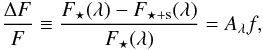 (2)where the contrast Aλ ≡ 1 − Fs(λ)/F⋆(λ) is a function of the passband. Similar approaches may be found in Désert et al. (2011a), Berta et al. (2011), and Carter et al. (2011).
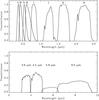 |
Fig. 1 The transmittance of the filter set adopted in this work. Top: the Johnson-Cousins-Glass photometric system. Bottom: the Spitzer/IRAC passbands. |
In the computation of the stellar flux, we assume that the stellar and the spot intensities vary according to the same quadratic limb-darkening law, namely ![Mathematical equation: \begin{equation} I(\lambda, \mu) = I(\lambda, 1) [1-u_{1 \lambda}(1-\mu) - u_{2 \lambda} (1-\mu)^{2}], \label{eq:limbdarkening} \end{equation}](/articles/aa/full_html/2012/03/aa17102-11/aa17102-11-eq36.png) (3)where I(λ,μ) is the specific intensity at wavelength λ, μ ≡ cosθ, with θ the angle between the normal to the stellar surface and the line of sight, and u1λ and u2λ are the limb-darkening coefficients (LDCs) at the given wavelength. Given the difference in the effective temperature, the LDCs of the unperturbed and the spotted photospheres are actually different, but in the modelling of the stellar and solar light curves they are assumed to be the same in order to simplify the treatment (see, e.g., Lanza et al. 2003, 2004). In our case, we have a maximum difference between the LDCs of ~30% in the U passband when considering main-sequence stars with an effective temperature in the range 3700–6000 K and spots with a temperature lower by 1250 K. In view of the advantages of assuming the same limb-darkening profile and the other uncertainties present in the problem, we neglect such a difference (cf. Sect. 2.2).
(3)where I(λ,μ) is the specific intensity at wavelength λ, μ ≡ cosθ, with θ the angle between the normal to the stellar surface and the line of sight, and u1λ and u2λ are the limb-darkening coefficients (LDCs) at the given wavelength. Given the difference in the effective temperature, the LDCs of the unperturbed and the spotted photospheres are actually different, but in the modelling of the stellar and solar light curves they are assumed to be the same in order to simplify the treatment (see, e.g., Lanza et al. 2003, 2004). In our case, we have a maximum difference between the LDCs of ~30% in the U passband when considering main-sequence stars with an effective temperature in the range 3700–6000 K and spots with a temperature lower by 1250 K. In view of the advantages of assuming the same limb-darkening profile and the other uncertainties present in the problem, we neglect such a difference (cf. Sect. 2.2).
The effect of the wavelength dependence of the limb darkening is shown in the case of CoRoT-2 by Czesla et al. (2009) using optical light curves at different wavelengths. The LDCs decrease from the U band to the infrared giving a more flat-bottomed transit at longer wavelengths with shorter ingress and egress profiles (see discussion in Sect. 6 and Fig. 11, Seager & Mallén-Ornelas 2003; Richardson et al. 2006) that can improve the determination of the transit parameters. Thus, even if we consider limb darkening in the derivation of the transit profiles, taking into account that it decreases towards longer wavelengths (see Table 1 in electronic form, Claret et al. 1995), its impact will not be so crucial, since our study is focused primarily on infrared passbands (see Deming et al. 2007; Carter et al. 2008; Berta et al. 2011).
The stellar microvariability may also be due to the presence of faculae, bright photospheric regions surrounding spots. They exhibit a centre-to-limb variation in their contrast and their brightness depends on size, position on the stellar disc, and wavelength. In the case of the Sun, they can produce a relative increase in the solar irradiance of ~10-3 (Fröhlich & Lean 2004) at the maximum of the 11-yr cycle. They are visible primarily in white light but their contrast with the unperturbed photosphere is lower in the near-infrared (Solanki & Unruh 1998; Fröhlich & Lean 2004) since it depends on λ-1 (Chapman & McGuire 1977). In the present study, we neglected their contribution since we are interested in the infrared bands where the facular effect may be considered less important. Moreover, the facular contribution to the optical flux variations is negligible in the case of stars significantly more active than the Sun (cf., e.g., Lanza et al. 2009,and references therein).
2.2. Effects of starspots on the apparent planetary radius
Starspots affect in two ways the stellar flux variations in a transit light curve. Spots that are not occulted by the planet produce a decrease in the out-of-transit flux of the star FOOT, which is the reference level to normalize the transit profile. Spots that are occulted during the transit produce a relative increase in the flux because the flux blocked by the planetary disc is lower than in the case of the unperturbed photosphere. The occultation of a starspot is therefore associated with a bump in the transit profile whose duration depends on the spot size and whose height depends on the spot contrast (e. g., Pont et al. 2007; Sing et al. 2011b). If we denote the flux during the transit as FIT, we have  (4)and
  (5)where ΔFs = Aλf0F⋆ is the flux decrease caused by the unocculted spots having a filling factor f0 (cf. Eq. (2)), and ⟨ I⋆(λ,μ) ⟩ is the specific intensity averaged over the portion of the stellar disc occulted by the planet of radius Rp. If we denote with fi the filling factor of the spots occulted during the transit when the planet’s centre is at the disc position μ along the transit chord, then
  (6)where ⟨ I⋆(λ,μ) ⟩ is the average of the specific intensity of the unperturbed photosphere over the area occulted by the planet, and ⟨ Is(λ,μ) ⟩ is the same quantity for the spotted photosphere. We note that Eq. (6) is valid because we have assumed that the spotted and unspotted photospheres have the same LDCs. If we define the relative transit profile at wavelength λ as D(λ,μ) ≡ 1 − FIT(λ,μ)/FOOT(λ), after some simple algebra we find that
 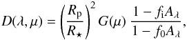 (7)where R⋆ is the radius of the star, and G(μ) is a function of the limb-darkening coefficients and the disc position μ of the planet during the transit, but does not depend on the spot distribution and temperature. If we define the unperturbed transit profile as
 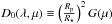 , the profile in the presence of spots is
 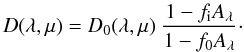 (8)If the ratio Rp/R⋆ ≲ 0.1, we can assume that ⟨ I⋆(λ,μ) ⟩ ≃ I⋆(λ,μ) (Mandel & Agol 2002) and the expression of the function G(μ) becomes particularly simple
 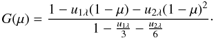 (9)In Eq. (7), the filling factor of the occulted spots fi is in general a function of the position of the centre of the planetary disc along the transit chord, while the filling factor of the out-of-transit spots f0 can be assumed to be constant because the visibility of those spots is modulated on timescales much longer than that of the transit, i.e., of the order of the stellar rotation period, which is generally several days. Moreover, when a geometric model is fitted to an observed transit profile, the bumps produced by occulted spots are excised from the data set to reduce their impact as much as possible. However, the capability of detecting the flux bump due to a particular spot depends on its size and contrast as well as on the accuracy and cadence of the photometry. If there is a more or less continuous background of spots along the transit chord, they cannot be individually resolved and the transit profile will appear to be symmetric and without any obvious indication of starspot perturbations. This is indeed the most dangerous case when fitting an observed transit profile. In this case, fi can be assumed to be constant during a given transit because otherwise we would have detected the individual spot bumps. If we assume that both f0 and fi are much less than unity, we can develop the denominator of Eq. (7) into a series and neglecting the second order terms in the filling factors, we find
 ![Mathematical equation: \begin{equation} D(\lambda, \mu) \simeq \left(\frac{R_{\rm p}}{R_{\rm \star}} \right)^{2} G(\mu) \left[ 1 - A_{\lambda}(f_{\rm i} - f_{0}) \right]. \label{eq:deficit_oc1} \end{equation}](/articles/aa/full_html/2012/03/aa17102-11/aa17102-11-eq66.png) (10)From Eq. (10), we see that the effects of the unocculted and occulted spots tend to compensate each other, although the filling factor of the occulted spots may generally be higher because starspots tend to appear at low or intermediate latitudes in Sun-like stars.
(10)From Eq. (10), we see that the effects of the unocculted and occulted spots tend to compensate each other, although the filling factor of the occulted spots may generally be higher because starspots tend to appear at low or intermediate latitudes in Sun-like stars.
Examined cases and their related real planetary systems.
An alternative interpretation of Eqs. (8) and (10) is that spots change the apparent relative radius of the planet (Rp/R⋆)a derived from the fitting of the transit profile (see Sect. 2.3) as ![Mathematical equation: \begin{equation} \left( \frac{R_{\rm p}}{R_{\star}} \right)_{\rm a} = ~\left( \frac{R_{\rm p}}{R_{\star}} \right) \sqrt{\frac{1-f_{\rm i}A_{\lambda }}{1-f_{0}A_{\lambda}}} \simeq \left( \frac{R_{\rm p}}{R_{\star}} \right) \left[ 1 - \frac{1}{2} A_{\lambda} (f_{i} - f_{0}) \right]. \end{equation}](/articles/aa/full_html/2012/03/aa17102-11/aa17102-11-eq75.png) (11)Therefore, the apparent variation in the planetary radius is
(11)Therefore, the apparent variation in the planetary radius is  (12)When radius measurements are available in two different passbands λ1 and λ2, we have
  (13)If the spot temperature is known, this equation can be used to derive the effective filling factor f ≡ fi − f0 from the apparent radius measurements in two well-separated passbands, e.g., in the U and the K passbands. If the spot temperature is not known, it can be derived when a third measurement is available in an additional passband, thereby removing the degeneracy between filling factors and contrast. However, the presence of a planetary atmosphere with a wavelength-dependent opacity can complicate the problem as we see in the final part of Sect. 3.2 in the case of HD 189733.
2.3. Effects of starspots on the determination of the orbital parameters
The perturbations of the transit profile due to starspots do not affect only the determination of the relative radius of the planet Rp/R⋆ but also the other geometrical parameters of the system and the limb-darkening coefficients. Most previous studies have considered only the radius variation (cf., e.g., Berta et al. 2011; Carter et al. 2011), but the impact on the other parameters can be significant. Czesla et al. (2009) explored the variation in the planetary radius and orbital inclination while fixing the semimajor axis of the orbit a, the stellar radius R⋆, and the limb-darkening coefficients u1 and u2 to the values of Alonso et al. (2008). In this way, they found that the radius of the planet is increased by ~3% by fitting the lower envelope of the transit profiles derived with their method. On the other hand, they found no significant correction in the inclination i of the orbital plane of the planet to the plane of the sky.
Contrast coefficients Aλ for each reference system in the different passbands.
A limitation of the approach by Czesla et al. (2009) is that by fixing the ratio a/R⋆, the duration of the transit tT fixes the inclination because  , where b = a/R⋆cosi is the impact parameter and Porb the orbital period. Since the effects of the spots on the duration of the transit are generally small, the inclination is not changed by fitting their unperturbed transit profile. Therefore, to perform a proper estimate of the systematic effects produced by occulted and unocculted spots, we cannot fix any of the system parameters in fitting the transit profile.
The unperturbed transit profile D0(λ,μ) can be derived from the lower envelope of the observed transit profiles if we can guess the minimum spot filling factor of the unocculted spots f0 min and of the spots occulted during transits fi min. From the lower envelope of the observed transits Dlow(λ,μ), we get an estimate of the unperturbed profile as  (14)Since fi min is a constant, the unperturbed profile does not contain any bumps due to the occultation of individual spots and is symmetric with respect to the mid-point of the transit.
We fit the unperturbed profile using an analytical model for the transit, e.g., that of Pál (2008). This has the advantage of providing analytic expressions for the derivatives of the transit profile D0 with respect to the transit parameters allowing us an efficient application of the Levenberg-Marquardt method to minimize the χ2 (Press et al. 1992). To minimize their mutual correlations, when running the best fitting procedure, we choose as free parameters  , b2, Rp/R⋆, and the limb darkening parameters u + ≡ u1 + u2 and u − ≡ u1 − u2 (see Pál 2008; Alonso et al. 2008,for a justification of the independence of this parameter set). The orbital period and the mid transit epoch are kept fixed in the fitting because they can be derived from the observation of a sufficiently long sequence of transits. Specifically, the profile distortions due to resolved occulted spots may affect the timing of individual transits, but the spot perturbations can be assumed to be random so that they increase the statistical error in the timing. Therefore, a sufficiently long time series can be used to derive an accurate value of Porb. We present an application of this method to estimate the impact of starspots on the fitting of the parameters of the system CoRoT-2 in Sect. 3.3.
3. Results
We focus our analysis on star temperature values ranging from the solar one (~5750 K) to that of an early M-type star and set the temperature difference between the star and the spot to 1250 K (see Berdyugina 2005). The synthetic spectra, for both the unperturbed photosphere and the spots, were chosen for solar metallicity and gravity, i.e. [M/H] ⊙ = 0.0 and log g⊙ = 4.44. To apply our results to real cases, we selected four systems with planets, i.e., CoRoT-12, with a transiting Jupiter-like planet orbiting around a G2V star (see Gillon et al. 2010), CoRoT-7, a K0V star (Léger et al. 2009; Queloz et al. 2009), HAT-P-20, a K7V star (Bakos et al. 2011), and GJ 436, a M2.5 dwarf star harbouring a transiting Neptune-mass planet (Butler et al. 2004). We list their properties in Table 1, where we give, from left to right, the spectral type, the selected temperature for the quiet photosphere and spot for the reference stars, the difference between the photosphere and spot temperatures, the real system with the name of the star we use for comparison, the stellar spectral type, the planetary radius and mass, and the reduction in flux at mid planetary transit, expressed in magnitudes (obtained as the square of the ratio of the planet radius to the star radius), respectively.
The contrast coefficients Aλ, giving the spot-induced flux variations for each of the examined cases (see Sect. 2.1), are obtained by choosing the spot filling factor of the out-of-transit spots, f0, ranging from 0.01 to 0.5 of the stellar disc surface (Berdyugina 2005) and are reported in Table 2. For G and early-K stars, the minimum flux perturbation occurs in the 8.0 μm Spitzer/IRAC passband, while the maximum occurs in the U passband because the spot contrast increases monotonically towards shorter wavelengths. In the case of late-K and M stars, the minimum flux perturbation occurs in the 4.5 μm and 3.6 μm Spitzer/IRAC passbands, respectively, due to molecular bands in the spectrum. These features are observed in the spectra of cooler stars, in both the optical and the infrared, and this results in a non-monotonous spectral variation in the correspondence of these bands. In this case, the unperturbed and spotted spectra do not behave as simply as power laws in the infrared domain as in the hotter cases.
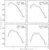 |
Fig. 2 Flux vs. wavelength for all the cases in Table 1. Solid lines plot the spectral distributions of the stellar unperturbed photospheres and dotted lines the spectral distributions of the star + spot systems with f0 = 0.5. In the top left we present the first case, in the top right the second case, in the bottom left the third case, and in the bottom right the fourth case. |
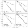 |
Fig. 3 Normalized FV/Fband vs. filling factor f0 for all the cases in Table 1 in the passbands I, K, and 8.0 μm. Different curves plot different ratios FV/FI, FV/FK, and FV/F8.0, as labelled. In the top left, we present the first case, in the top right the second case, in the bottom left the third case, and in the bottom right the fourth case. |
In Fig. 2, we plot the system flux versus (vs.) wavelength for all the cases, for a given filling factor of the out-of-transit spots. The solid curve represents the spectrum of the unperturbed photosphere and the dotted line the spectral distribution of the system “star + spots”. We plot a case with an extreme filling factor (f0 = 0.5) to make the effect of the spots clearly evident. The spot perturbation decreases with increasing wavelength, although the details of the variation depends on the stellar effective temperature.
In Fig. 3, we plot the variations in the normalized ratios FV/Fband vs. the filling factor f0, where Fband is computed in three specified passbands (I,K, and 8.0 μm), with the purpose of understanding the extent to which the stellar magnetic activity may produce a variation in the colours of the star (this graph is discussed in detail in Sect. 3.1).
These results suggest that the effect of stellar activity on colour has to be taken into account if we analyse the photometric signals even of a moderately active star (comparable with or slightly more active than our Sun). The effects are on both stellar colours (discussed in Sect. 3.1) and the determination of the radius of the planet (discussed in Sect. 3.2).
3.1. Influence of stellar activity on stellar colours and the characterization of a single light curve dip
If we consider the first and the fourth cases in Table 1 (i.e., the hottest and the coolest host stars), by fixing the filling factor f0 to 1% (i.e., larger than in the solar case, but comparable to those observed in late-type moderately active stars), we can compute the relative variation in the system flux (ΔF/F) in the U and K-bands, to compare the influence of stellar activity in the optical and infrared passbands.
For the first case (T⋆ = 5750 K, ΔT = 1250 K), we derive the variations in the U-band and in the K-band, respectively, to be  (15)For the fourth case (T⋆ = 3750 K, ΔT = 1250 K), we derive the following values in the U-band and in the the K-band, respectively,
  (16)The decrease in flux caused by a spot filling factor of 0.01 is comparable to the decrease produced by the transit of a Jupiter-sized planet in front of the stellar disc. We can compare the obtained reductions in flux of the system due to stellar magnetic activity, using the information in Table 2, with the decrease in magnitude due to the transit of a planet, reported in Table 1.
Variations in the colour of the system for all the cases. Top: computed for f0 = 0.1. Bottom: computed for f0 = 0.01.
Our results indicate that it is easier to identify the transit of a Jupiter-like planet by analysing the light curve of the system in the K-band, while it may be more problematic in the U-band. The detection of a smaller planet is more challenging, in both the U and the K-band, since the photometric signal corresponding to the transit of such a planet is, as expected, smaller than the effect of the magnetic activity of its parent star. Fortunately, other properties of the variations, such as timescales or colour dependences, may help in understanding the origin of the variations.
The transit of a spot or a group of spots (or an active region in general) on the star surface induces a colour variation in the star. Since spots are cooler than the stellar photosphere, the colour indices are higher. In principle, we can infer the activity of a star by monitoring the variation in the colour for some specified wavebands. Star colours depend on the ratio of the fluxes in two selected passbands. For this purpose, we compute the ratio of the system fluxes in the optical and the infrared passbands, for all the four template cases represented by FV/FI, FV/FK, and FV/F8.0. In Table 3, we report the variation in FV/Fband in the different bands, by fixing the filling factor f0 to either 0.1 and to 0.01, respectively. The first column shows the filling factors and the enumeration of the cases, and the subsequent columns show the changes in FV/FI, in FV/FK, and in FV/F8.0, respectively. The behaviour of the star flux ratios vs. spot filling factor of the unocculted spots are plotted in Fig. 3, where the ratios decrease as the spot filling factor increases.
The transit of a planet without atmosphere induces a relative decrease in the stellar flux that depends on the mean wavelength of the passband owing to the wavelength dependence of the stellar limb darkening. For the present application, we consider the central transit (b = 0) of a small planet (Rp/R⋆) ≲ 0.1, with the quadratic limb-darkening law of Eq. (3). We derive the ratio ℛ of the relative depths of the transit at the mean wavelengths of two different passbands, say U and K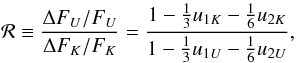 (17)where u1U, u2U, u1K, and u2K are the limb-darkening coefficients in the U and K passbands, derived from, e.g., Diaz-Cordoves et al. (1995) and Claret et al. (1995), respectively. For the first case, we find that ℛ = 1.298, while for the fourth case, ℛ = 1.197. This is significantly smaller than expected in the case of the variations induced by dark spots (cf. (15) and (16)). The flux in the K passband coming from the night side of the planet during the transit is neglected because the planet temperature, even for the most strongly irradiated objects, is always lower than ~2000 K, which is remarkably lower than the temperature of the starspots.
Considering Eq. (2), we find that the ratio of the variations induced by starspots is  (18)For a stellar effective temperature of 5750 K, this is always significantly greater than 1.3, except for very cool spots, i.e., ΔT ≥ 2100 K. Spots so cool are generally not observed in active stars (see, e.g., Berdyugina 2005). For the Sun as a star, ΔT ≃ 500–600 K because sunspot irradiance is dominated by the penumbral regions (cf., e.g., Lanza et al. 2004,and references therein). For a star with T⋆ = 3750 K, a spot temperature deficit ΔT ≥ 1500 K is required to produce a ℛs that is comparable to that of a planetary transit, which is also unlikely for such a cool star (see, e.g., Berdyugina 2005; Zboril 2003).
In conclusion, even for an individual light-curve dip, we are able to compare the variation in the depths in the optical and infrared passbands to discriminate between an effect induced by spot activity and a planetary transit, because the ratio ℛ is in the range 1.7–3.0 in the former case (see the ratio of relations in Eqs. (15) and (16), for a typical ΔT = 1250 K), while it is around 1.2–1.3 in the latter case.
The timescales of the stellar flux variability and the transit are generally quite different, since the former may range from weeks to months as in the case of the Sun (Lanza et al. 2003, 2007), while the latter has a duration ranging from a few hours to a few tens of hours. However, there are situations in which the timescales can be comparable, e.g., for a young Sun-like star with a rotation period of, say, 1–2 days transited by a planet at the distance of ~1 AU, whose transit duration is of the order of ~10–15 h. In this case, a discrimination of the origin of the light dip based on timescales is infeasible, while our approach is still applicable if simultaneous multiwavelength observations are available. Our method can be applied in principle even to a single event. This can be very useful in the case of planets with orbital periods of several tens or hundreds of days.
The photometric precision currently achievable from the ground in the near-infrared is generally sufficient for an application of the present method, provided that the photometric variations are at least 0.005 − 0.01 mag. Croll et al. (2011) acquired photometry with a standard deviation of σ ≃ 5 × 10⁻³ mag in the J (1.25 μm) and the K (2.15 μm) bandpasses using the WIRCam at the 3.5-m CFHT, while Tofflemire et al. (2012) reached a photometric stability of 3.9 × 10⁻³ mag in one hour and 5.1 × 10⁻³ mag in one night in the Ks passband at 2.224 μm observing stable M-type stars. However, the situation is remarkably different in the mid and far infrared passbands.
From space, the Warm Spitzer mission has reached a statistical error of 450 ppm (parts per million) per minute, observing GJ 1214 for 12 s at 3.6 μm (Gillon et al. 2011). However, the infrared (IR) observations are affected by systematic effects that may compromise the measurements because these effects induce flux variations comparable to the depth of a planetary transit. For example, the 3.6 and 4.5 μm Spitzer/IRAC channels (InSb detectors) are affected by the pixel-phase effect (Reach et al. 2005; Charbonneau et al. 2005; Morales-Calderón et al. 2006; Knutson et al. 2008) due to the telescope jitter and intra-pixel variation in the sensitivity of the detector, which may cause a flux peak-to-peak amplitude of up to ~1% (Beaulieu et al. 2008; Hébrard et al. 2010) or even higher (Désert et al. 2011b; Fressin et al. 2011), according to the exposure time. The light curves of the 5.8 and 8.0 μm channels (Si:As detectors) follow non-linear trends with time, called the ramp effect (Deming et al. 2006; Knutson et al. 2007a), caused by the trapping of electrons by the detector impurities (see Agol et al. 2010 for further details), which produce mmag level flux variations in photometry. They can reach up to ~10% for the least illuminated pixels over 33 h (Agol et al. 2010), and increase over time (Machalek et al. 2008). The correction of these instrumental systematics and artifacts is particularly relevant for future infrared missions, such as JWST, since the same Si:As technology, present in the last two Spitzer/IRAC channels, will be adopted for MIRI (Mid-Infrared Instrument, see Gardner et al. 2006).
In this study, we intend instead to emphasize the importance of a broad-band monitoring of stars hosting planets from the visible, at the shortest wavelength as possible, to IR. Simultaneous observations, from optical to infrared wavebands, allow us to more clearly understand the role of stellar magnetic activity in the analysis of a transiting planet light curve by comparing the ratios ℛ derived in Eqs. (17) and (18), as stated before.
3.2. Influence of stellar activity on planetary radius determination
We apply the simple formulae of Sect. 2.2 to evaluate the variation in the apparent planetary radius in the presence of stellar activity, assuming that the other parameters are not affected. The effect of the activity on the simultaneous determination of the radius and the orbital parameters is illustrated in Sect. 3.3. The plots in Fig. 4, ΔRp/Rp vs. wavelength, give us the overestimate of Rp if the effect of unocculted starspots is neglected for our four reference cases. We find a relation both between ΔRp/Rp and the wavelength and between ΔRp/Rp and the stellar activity, i.e. increasing the filling factor of the out-of-transit spots f0 the dashed curves shift upwards and the variation decreases towards longer wavelengths. The filled circles on the plot indicate the correction to the observed planetary radius that we have to apply to get the true radius of the planet for the assumed spot temperature and filling factors (see below).
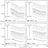 |
Fig. 4 Relative variation in the apparent planetary radius vs. wavelength for all the examined planetary systems. In the top left, we present the results for CoRoT-12b, in the top right for CoRoT-7b, in the bottom left for HAT-P-20b, and in the bottom right for GJ 436b, assuming various levels of activity. The dashed curves, from the bottom to the top, correspond to increasing filling factor values, as indicated on the left of each plot. The solid curves refer to the activity levels as actually estimated for the specified systems. The filled points indicate the position of the observed planets, as described in the text. |
In the top left panel of Fig. 4, we present the result for CoRoT-12. We assumed a filling factor of f0 = 0.03 (the solid line in the panel) by inferring the flux variation from the CoRoT light curve of Fig. 1 in Gillon et al. (2010) and then derived the contrast coefficients from the first row of Table 2.
The top right panel of Fig. 4 shows ΔRp/Rp vs. wavelength for CoRoT-7. The spot filling factor value is f0 = 0.04 by deducing it from the optical flux variability reported in Lanza et al. (2010).
For HAT-P-20, the outcomes are shown in the bottom left panel of Fig. 4. We set f0 = 0.01 as derived by the magnitude variations in the stellar flux for the R-band shown in Fig. 1 in Bakos et al. (2011). The dependences of ΔRp/Rp on both the wavelength and the stellar activity are also clearly visible for this planet too, even though the curves tend to become flat.
The bottom right panel of Fig. 4 shows the result for GJ 436. The star is a relatively quiet source showing photometric variations of the order of the millimag (Butler et al. 2004). Demory et al. (2007) found that the photometric irregularities in the light curve of GJ 436, detected with the EULER Telescope, are caused by an unocculted starspot and they computed a spot filling factor of 1%, which is compatible with the dispersion in the HARPS radial velocity. Thus, we set f0 = 0.01.
Relative variation in planetary radius and radius uncertainty computed at optical wavelengths for the analysed stars.
Corrected planetary radii in the optical and Spitzer wavebands for three notable examples: HD 209458b, HD 189733b, and GJ 436b.
In Table 4, we list the obtained results taking into account the above filling factor values: from the left to the right, the planet name, ΔRp/Rp, and the relative variation in the radius uncertainty ΔErr, which is the ratio of the computed ΔRp with respect to the uncertainties quoted in the literature4 (see also Table 1). By a simple check, we note that the largest values of ΔRp/Rp and ΔErr occur for the most active star within our sample, i.e. CoRoT-7 with f0 = 0.04, while the lowest values are found for the coolest and less active stars, i.e. HAT-P-20 and GJ 436 with f0 = 0.01 in both cases. For CoRoT-7b, we compute an overestimate of the planetary radius, ΔRp, of about 180 km at optical wavelengths (with a relative variation in the radius uncertainty of about 31%), while in the K-band it is about 92 km and even smaller at Spitzer/IRAC wavebands (at 3.6 μm, ΔRp ≃ 84 km and at 8.0 μm ΔRp ≃ 75 km). This decrease in ΔRp as wavelength increases is exhibited by the other examined planetary systems and could be misinterpreted as evidence of a planetary atmosphere with a wavelength-dependent absorption. Since ΔRp is proportional to the planetary radius, we obtain the largest ΔRp for CoRoT-12b (ΔRp ≃ 1180 km at optical wavelengths) with a Jupiter-like planet and the lowest for GJ 436b (ΔRp ≃ 130 km in the optical) with its super-Earth planet. Nevertheless, all the radius increments calculated in this work fall inside the error bars quoted in the literature, thus no correction to the presently determined planetary parameters is required. We see that for each value of the filling factor, the curves seem to start nearly at the same level (i.e. ΔRp/Rp ≃ 0.005 for f0 = 0.01 and ΔRp/Rp ≃ 0.24 for f0 = 0.5), independently of the stellar photospheric temperature. Their trends remain monotonic but their slopes decrease towards cooler photospheric temperatures (cf. GJ 436, in the bottom right panel of Fig. 4). This indicates that the overestimate of the planetary radius depends on the wavelength, with the dependence being steeper for solar-type stars and flatter for later spectral types.
Specifically considering the Spitzer passbands, we apply the method described above to two of the most studied planetary systems: HD 209458 and HD 189733. These systems have been the objects of intense study at a wide range of wavelengths from the optical with the HST (Brown et al. 2001; Knutson et al. 2007b; Pont et al. 2007; Sing et al. 2011b) to the infrared with the Spitzer satellite (Richardson et al. 2006; Ehrenreich et al. 2007; Tinetti et al. 2007b; Beaulieu et al. 2008, 2010; Désert et al. 2011a), also as targets for transmission spectroscopy thanks to their brightness.
In Table 5, we report the results and present the corresponding ones for GJ 436b for comparison. In all cases, we have considered two different filling factor values for the unocculted spots: one is that derived as described below, while the other one is given for comparison (indicated in parenthesis in the table).
HD 209458 is an almost quiet solar-like G0V star and the calculations have been made considering the two configurations f0 = 0.004 and f0 = 0.03. The former f0 value was estimated assuming a circular spot with an average radius of 4.5 × 10⁴ km as in the model proposed by Silva (2003) to fit the distortion of a single transit of HD 209458 observed by HST. HD 189733 is an active early-K star with f0 = 0.03 (Désert et al. 2011a). To derive the quantities, we interpolated the BaSeL spectra at temperatures corresponding to the stellar effective temperatures (Teff = 6000 K and Teff = 5000 K for HD 209458 and HD 189733, respectively) and assuming ΔT = 1250 K for both cases. The table also lists the measured planetary radius and the related uncertainty, as reported in the literature.
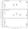 |
Fig. 5 Corrected planetary radii vs. Wavelength. Top panel, HD 209458b. Middle panel, HD 189733b. Bottom panel, GJ 436b. The open ° circle indicates the planetary radius inferred from the literature, the × cross the corrected radius with f0 = 0.004 for HD 209458b and f0 = 0.01 for HD 189733b and GJ 436b and the ∗ asterisk the corrected radius with f0 = 0.03. The plotted points are shifted horizontally for an easier identification. |
In Fig. 5, we show the corrected planetary radii vs. wavelength, along with the uncertainties reported in the literature. The adopted stellar radii are RHD 209458 = 1.146 R⊙ (Brown et al. 2001), RHD 189733 = 0.788 R⊙ (Baines et al. 2008), RGJ 436 = 0.464 R⊙ (Torres 2007), respectively. The most active star (i.e. HD 189733) shows significant discrepancies between the planet radius inferred from the literature and the one determined here; this is an expected result since ΔRp ∝ f (see Eq. (12) in Sect. 2.2) and may have interesting consequences if one wishes to characterize the planet atmosphere through transmission spectroscopy. Similarly, in the quiet cases, even though our corrections are within the error bars reported in the literature (of the order of the hundreth or of the thousandth, see Table 5), they may become significant for the determination of the physical properties of similar exoplanets. The wavelength dependence of the apparent radius of HD 189733b in the optical passbands was observed by Sing et al. (2011b). They used an approach similar to that of Sect. 2.2 and concluded that the variation in Rp/R⋆ vs. wavelength λ cannot be reproduced by an equation analogous to Eq. (13), thus providing evidence of the wavelength dependence of the planetary atmospheric absorption.
3.3. Effects of stellar activity on orbital parameters
To illustrate the impact of starspots on the determination of all the transit parameters, we considered the case of CoRoT-2 because it had been studied by Czesla et al. (2009) and its spot activity had been investigated in detail. Since we are interested in the systematic errors produced by starspots, we simulated a noiseless transit profile by adopting the time sampling and the parameters derived by Alonso et al. (2008), and applied Eq. (8) with spot filling factors estimated from Lanza et al. (2009) for the out-of-transit light curve and Silva-Valio et al. (2010) for the transit light curve, respectively. To derive the transit profile to be fitted with their model, Alonso et al. (2008) averaged all the transits observed by CoRoT. Therefore, we assumed that the spot perturbation corresponds to the average values of the filling factors f0 and fi as derived from the modelling of the out-of-transit and the transit light curves, respectively. By fitting the light curve of CoRoT-2 outside transits, Lanza et al. (2009) derived an average spot filling factor f0 = 0.07 by adopting a spot contrast in the CoRoT white passband of ALANZA = 0.665. On the other hand, Silva-Valio et al. (2010) found an average filling factor of fi = 0.15 for a spot contrast of ASILVA = 0.55. Multiplying it by the ratio ALANZA/ASILVA, we converted it into the scale of Lanza et al. (2009), giving fi = 0.18. With those values of the filling factors and Aλ = 0.665, we computed the unperturbed transit profile D0 from Eq. (8) and then fitted it with the Levenberg-Marquardt algorithm as implemented in the IDL procedure lmfit. The unperturbed transit profile and its best fit are plotted in Fig. 6 together with the initial profile assumed to be perturbed by the effects of the spots. The best fit has a reduced χ2 = 1.29 computed by assuming a relative standard deviation of the simulated data of 1.09 × 10⁻⁴ as in the case of the CoRoT data analysed by Alonso et al. (2008). The best-fit parameters and their standard deviations derived from the covariance matrix with the above assumed data standard deviation (see Press et al. 1992,Sect. 15.4) are a/R⋆ = 6.76 ± 0.03, Rp/R⋆ = 0.1726 ± 0.00006,  , u1 = 0.40 ± 0.04, and u2 = 0.097 ± 0.04.
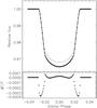 |
Fig. 6 Top panel: the synthetic light curve of the transit of CoRoT-2 computed with the parameters in Table 1 of Alonso et al. (2008) (dashed line) together with the unperturbed profile obtained from Eq. (8) (diamonds) and the corresponding best fit (solid line). The flux is measured in units of the out-of-transit flux level in all the cases. Bottom panel: the residuals of the best fit to the unperturbed transit profile in relative flux units vs. the orbital phase. |
We confirmed that the radius variation is close to that estimated with the simple approach of Sect. 2.2 because the depth of the profile at mid transit gives the principal constraint on the relative radius. However, in contrast to the results of Czesla et al. (2009), we found that the relative semimajor axis a/R⋆ and the inclination i are also affected, with variations that exceed three standard deviations for both parameters (cf. Table 1 of Alonso et al. 2008). We note that the transit duration tT is the same in our model for both the unperturbed and the perturbed transit profiles. Therefore, the variations in a/R⋆ and i combine with each other to ensure that tT remains practically constant (see Sect. 2.3). The variation in a/R⋆ has an impact on the measurement of the density of the star (cf. Seager & Mallén-Ornelas 2003; Sozzetti et al. 2007) that, together with its effective temperature, is used to derive its position on the H-R diagram and hence its age from the isochrones. We did not consider this application any further because it was beyond the scope of the present work, but conclude that starspot effects cannot be neglected in the derivation of the stellar density from the transit fitting in the case of active planetary hosts.
The limb-darkening parameters were not significantly affected by the stellar variability. The small systematic deviations in the ingress and egress of the profile do not lead to any significant adjustment of the limb darkening (cf. upper and lower panels of Fig. 6).
Other stellar parameters can be affected by starspots, notably the effective temperature Teff. This problem was discussed in detail for CoRoT-2 by Guillot & Havel (2011) who found that the effect of spots is that of increasing the uncertainty in the determination of Teff because of their changing covering factor along the activity cycle of the star. We did not consider these aspects further because we focused on the parameters directly related to the modelling of the transit light curve.
4. Conclusions
We have demonstrated that the observation of stars moderately active simultaneously in the optical and the near-infrared passbands allows us to discriminate between planetary transits and activity-induced variations, unless starspots are 2000–2500 K cooler than the unperturbed photosphere, which is generally not observed in main-sequence stars. This approach can be applied to individual light-curve dips observed with a signal-to-noise ratio of ≈ 10–15% of the flux variations in two well-separated passbands, e.g., U and K, and does not require a characterization of the stellar microvariability timescales, which would require observations extended for at least 2–3 stellar rotations.
Moreover, infrared observations are important for the derivation of the planetary radius and accordingly of the planetary density. The correction for the effects of starspots is necessary to avoid systematic errors in transmission spectroscopy, especially when comparing the planetary radii at optical and infrared passbands. A correct determination of the planetary radius enables us to perform a more accurate study of the planetary atmosphere and its composition in the framework of transmission and reflection spectroscopy. We provide simple formulae, tabulations, and graphics useful to estimate the starspot perturbation for typical transiting systems. Moreover, we have found that starspots may affect the relative semimajor axis a/R⋆ and the inclination i derived by transit fitting. This may have a non-negligible impact on the determination of the stellar density, especially when optical light curves are used. Near-infrared light curves are less affected, but the effect may still be significant for very active stars.
A simultaneous broad-band photometric observation, from visible to infrared wavelengths, of a significant sample of stars might itself be a relevant tool for identifying and characterizing their stellar activity, allowing us to disentagle its contribution from planetary transit signals. Such observations are useful to derive relevant and accurate information about the primary parameters of the planets (as already suggested by Jha et al. 2000) and the physical properties of their atmospheres, providing tighter constraints of temperatures and chemical compositions.
The EChO mission has been selected for the assessment phase for the medium-class mission, to be launched in the period 2020–2022 by ESA.
Throughout this section, we present the results achieved in the literature by comparing the planet-to-star radius ratio of each source, so as to use quantities directly related to the observations, avoiding any inconsistency due to the use of different stellar radii. Where needed, we compute the Rp/R⋆ ratio by using the stellar radius adopted in the relevant paper.
See site http://exoplanet.eu/index.php
Acknowledgments
The authors gratefully acknowledge an anonymous referee and the A&A editor Dr. T. Guillot for their valuable comments on a previous version of this manuscript that greatly helped to improve their work. Support for this research has been provided by the contract PRIN-INAF (P.I.: Lanza). We acknowledge contribution from ASI (agreement I/044/10/0).
References
- Agol, E., Cowan, N. B., Knutson, H. A., et al. 2010, ApJ, 721, 1861 [NASA ADS] [CrossRef] [Google Scholar]
- Aigrain, S., & Irwin, M. 2004, MNRAS, 350, 331 [NASA ADS] [CrossRef] [Google Scholar]
- Alonso, R., Auvergne, M., Baglin, A., et al. 2008, A&A, 482, L21 [NASA ADS] [CrossRef] [EDP Sciences] [Google Scholar]
- Baines, E. K., McAlister, H. A., ten Brummelaar, T. A., et al. 2008, ApJ, 680, 728 [NASA ADS] [CrossRef] [Google Scholar]
- Bakos, G. Á., Knutson, H., Pont, F., et al. 2006, ApJ, 650, 1160 [NASA ADS] [CrossRef] [Google Scholar]
- Bakos, G. Á., Hartman, J., Torres, G., et al. 2011, ApJ, 742, 116 [NASA ADS] [CrossRef] [Google Scholar]
- Bean, J. L., Benedict, G. F., Charbonneau, D., et al. 2008, A&A, 486, 1039 [NASA ADS] [CrossRef] [EDP Sciences] [Google Scholar]
- Beaulieu, J. P., Carey, S., Ribas, I., & Tinetti, G. 2008, ApJ, 677, 1343 [NASA ADS] [CrossRef] [Google Scholar]
- Beaulieu, J. P., Kipping, D. M., Batista, V., et al. 2010, MNRAS, 409, 963 [NASA ADS] [CrossRef] [Google Scholar]
- Berdyugina, S. V. 2005, Liv. Rev. Sol. Phys., 2, 8 [Google Scholar]
- Berta, Z. K., Charbonneau, D., Bean, J., et al. 2011, ApJ, 736, 12 [NASA ADS] [CrossRef] [Google Scholar]
- Bessell, M. S. 1990, PASP, 102, 1181 [NASA ADS] [CrossRef] [Google Scholar]
- Bessell, M. S., & Brett, J. M. 1988, PASP, 100, 1134 [NASA ADS] [CrossRef] [Google Scholar]
- Bessell, M. S., Brett, J. M., Wood, P. R., & Scholz, M. 1989, A&AS, 77, 1 [NASA ADS] [Google Scholar]
- Bessell, M. S., Brett, J. M., Scholz, M., & Wood, P. R. 1991, A&AS, 89, 335 [NASA ADS] [Google Scholar]
- Bonomo, A. S., & Lanza, A. F. 2008, A&A, 482, 341 [NASA ADS] [CrossRef] [EDP Sciences] [Google Scholar]
- Bonomo, A. S., Aigrain, S., Bordé, P., & Lanza, A. F. 2009, A&A, 495, 647 [NASA ADS] [CrossRef] [EDP Sciences] [Google Scholar]
- Bouchy, F., Udry, S., Mayor, M., et al. 2005, A&A, 444, L15 [NASA ADS] [CrossRef] [EDP Sciences] [Google Scholar]
- Brown, T. M. 2001, ApJ, 553, 1006 [NASA ADS] [CrossRef] [Google Scholar]
- Brown, T. M., Charbonneau, D., Gilliland, R. L., Noyes, R. W., & Burrows, A. 2001, ApJ, 552, 699 [NASA ADS] [CrossRef] [Google Scholar]
- Butler, R. P., Vogt, S. S., Marcy, G. W., et al. 2004, ApJ, 617, 580 [NASA ADS] [CrossRef] [Google Scholar]
- Cameron, A. C., Horne, K., Penny, A., & James, D. 1999, Nature, 402, 751 [NASA ADS] [CrossRef] [Google Scholar]
- Carter, J. A., Yee, J. C., Eastman, J., Gaudi, B. S., & Winn, J. N. 2008, ApJ, 689, 499 [NASA ADS] [CrossRef] [Google Scholar]
- Carter, J. A., Winn, J. N., Holman, M. J., et al. 2011, ApJ, 730, 82 [NASA ADS] [CrossRef] [Google Scholar]
- Chapman, G. A., & McGuire, T. E. 1977, ApJ, 217, 657 [NASA ADS] [CrossRef] [Google Scholar]
- Charbonneau, D., Noyes, R. W., Korzennik, S. G., et al. 1999, ApJ, 522, L145 [NASA ADS] [CrossRef] [Google Scholar]
- Charbonneau, D., Brown, T. M., Noyes, R. W., & Gilliland, R. L. 2002, ApJ, 568, 377 [NASA ADS] [CrossRef] [Google Scholar]
- Charbonneau, D., Allen, L. E., Megeath, S. T., et al. 2005, ApJ, 626, 523 [NASA ADS] [CrossRef] [Google Scholar]
- Charbonneau, D., Berta, Z. K., Irwin, J., et al. 2009, Nature, 462, 891 [NASA ADS] [CrossRef] [PubMed] [Google Scholar]
- Claret, A., Diaz-Cordoves, J., & Gimenez, A. 1995, A&AS, 114, 247 [NASA ADS] [Google Scholar]
- Croll, B., Albert, L., Jayawardhana, R., et al. 2011, ApJ, 736, 78 [NASA ADS] [CrossRef] [Google Scholar]
- Czesla, S., Huber, K. F., Wolter, U., Schröter, S., & Schmitt, J. H. M. M. 2009, A&A, 505, 1277 [NASA ADS] [CrossRef] [EDP Sciences] [Google Scholar]
- Deming, D., Harrington, J., Seager, S., & Richardson, L. J. 2006, ApJ, 644, 560 [NASA ADS] [CrossRef] [MathSciNet] [Google Scholar]
- Deming, D., Harrington, J., Laughlin, G., et al. 2007, ApJ, 667, L199 [NASA ADS] [CrossRef] [Google Scholar]
- Deming, D., Agol, E., Ford, E., et al. 2009, in Astronomy, 2010, astro2010: The Astronomy and Astrophysics Decadal Survey, 63 [Google Scholar]
- Demory, B., Gillon, M., Barman, T., et al. 2007, A&A, 475, 1125 [NASA ADS] [CrossRef] [EDP Sciences] [Google Scholar]
- Désert, J., Lecavelier des Etangs, A., Hébrard, G., et al. 2009, ApJ, 699, 478 [NASA ADS] [CrossRef] [Google Scholar]
- Désert, J., Sing, D., Vidal-Madjar, A., et al. 2011a, A&A, 526, A12 [NASA ADS] [CrossRef] [EDP Sciences] [Google Scholar]
- Désert, J.-M., Bean, J., Miller-Ricci Kempton, E., et al. 2011b, ApJ, 731, L40 [NASA ADS] [CrossRef] [Google Scholar]
- Diaz-Cordoves, J., Claret, A., & Gimenez, A. 1995, A&AS, 110, 329 [NASA ADS] [Google Scholar]
- Ehrenreich, D., Hébrard, G., Lecavelier des Etangs, A., et al. 2007, ApJ, 668, L179 [NASA ADS] [CrossRef] [Google Scholar]
- Fluks, M. A., Plez, B., The, P. S., et al. 1994, A&AS, 105, 311 [NASA ADS] [Google Scholar]
- Fressin, F., Torres, G., Desert, J.-M., et al. 2011, ApJS, 197, 5 [NASA ADS] [CrossRef] [Google Scholar]
- Fröhlich, C., & Lean, J. 2004, A&ARv, 12, 273 [Google Scholar]
- Gardner, J. P., Mather, J. C., Clampin, M., et al. 2006, Space Sci. Rev., 123, 485 [NASA ADS] [CrossRef] [Google Scholar]
- Gibson, N. P., Pont, F., & Aigrain, S. 2011, MNRAS, 411, 2199 [NASA ADS] [CrossRef] [Google Scholar]
- Gillon, M., Hatzes, A., Csizmadia, S., et al. 2010, A&A, 520, A97 [NASA ADS] [CrossRef] [EDP Sciences] [Google Scholar]
- Gillon, M., Bonfils, X., Demory, B.-O., et al. 2011, A&A, 525, A32 [NASA ADS] [CrossRef] [EDP Sciences] [Google Scholar]
- Guillot, T., & Havel, M. 2011, A&A, 527, A20 [NASA ADS] [CrossRef] [EDP Sciences] [Google Scholar]
- Hébrard, G., Désert, J.-M., Díaz, R. F., et al. 2010, A&A, 516, A95 [NASA ADS] [CrossRef] [EDP Sciences] [Google Scholar]
- Hubbard, W. B., Fortney, J. J., Lunine, J. I., et al. 2001, ApJ, 560, 413 [NASA ADS] [CrossRef] [Google Scholar]
- Huber, K. F., Czesla, S., Wolter, U., & Schmitt, J. H. M. M. 2010, A&A, 514, A39 [NASA ADS] [CrossRef] [EDP Sciences] [Google Scholar]
- Jha, S., Charbonneau, D., Garnavich, P. M., et al. 2000, ApJ, 540, L45 [NASA ADS] [CrossRef] [Google Scholar]
- Knutson, H. A., Charbonneau, D., Allen, L. E., et al. 2007a, Nature, 447, 183 [NASA ADS] [CrossRef] [PubMed] [Google Scholar]
- Knutson, H. A., Charbonneau, D., Noyes, R. W., Brown, T. M., & Gilliland, R. L. 2007b, ApJ, 655, 564 [NASA ADS] [CrossRef] [Google Scholar]
- Knutson, H. A., Charbonneau, D., Allen, L. E., Burrows, A., & Megeath, S. T. 2008, ApJ, 673, 526 [NASA ADS] [CrossRef] [Google Scholar]
- Lanza, A. F., Rodonò, M., Pagano, I., Barge, P., & Llebaria, A. 2003, A&A, 403, 1135 [NASA ADS] [CrossRef] [EDP Sciences] [Google Scholar]
- Lanza, A. F., Rodonò, M., & Pagano, I. 2004, A&A, 425, 707 [NASA ADS] [CrossRef] [EDP Sciences] [Google Scholar]
- Lanza, A. F., Bonomo, A. S., & Rodonò, M. 2007, A&A, 464, 741 [NASA ADS] [CrossRef] [EDP Sciences] [Google Scholar]
- Lanza, A. F., Pagano, I., Leto, G., et al. 2009, A&A, 493, 193 [NASA ADS] [CrossRef] [EDP Sciences] [Google Scholar]
- Lanza, A. F., Bonomo, A. S., Moutou, C., et al. 2010, A&A, 520, A53 [NASA ADS] [CrossRef] [EDP Sciences] [Google Scholar]
- Léger, A., Rouan, D., Schneider, J., et al. 2009, A&A, 506, 287 [NASA ADS] [CrossRef] [EDP Sciences] [MathSciNet] [Google Scholar]
- Lejeune, T., Cuisinier, F., & Buser, R. 1997, A&AS, 125, 229 [NASA ADS] [CrossRef] [EDP Sciences] [Google Scholar]
- Lejeune, T., Cuisinier, F., & Buser, R. 1998, A&AS, 130, 65 [NASA ADS] [CrossRef] [EDP Sciences] [Google Scholar]
- Machalek, P., McCullough, P. R., Burke, C. J., et al. 2008, ApJ, 684, 1427 [NASA ADS] [CrossRef] [Google Scholar]
- Mandel, K., & Agol, E. 2002, ApJ, 580, L171 [NASA ADS] [CrossRef] [Google Scholar]
- Marino, G., Rodonó, M., Leto, G., & Cutispoto, G. 1999, A&A, 352, 189 [NASA ADS] [Google Scholar]
- Miller-Ricci, E., & Fortney, J. J. 2010, ApJ, 716, L74 [NASA ADS] [CrossRef] [Google Scholar]
- Morales-Calderón, M., Stauffer, J. R., Kirkpatrick, J. D., et al. 2006, ApJ, 653, 1454 [NASA ADS] [CrossRef] [Google Scholar]
- Moutou, C., Pont, F., Barge, P., et al. 2005, A&A, 437, 355 [NASA ADS] [CrossRef] [EDP Sciences] [Google Scholar]
- Nutzman, P., & Charbonneau, D. 2008, PASP, 120, 317 [NASA ADS] [CrossRef] [Google Scholar]
- Pál, A. 2008, MNRAS, 390, 281 [NASA ADS] [CrossRef] [Google Scholar]
- Pallé, E., Zapatero Osorio, M. R., & García Muñoz, A. 2011, ApJ, 728, 19 [NASA ADS] [CrossRef] [Google Scholar]
- Pont, F., Gilliland, R. L., Moutou, C., et al. 2007, A&A, 476, 1347 [NASA ADS] [CrossRef] [EDP Sciences] [MathSciNet] [Google Scholar]
- Pont, F., Knutson, H., Gilliland, R. L., Moutou, C., & Charbonneau, D. 2008, MNRAS, 385, 109 [NASA ADS] [CrossRef] [Google Scholar]
- Press, W. H., Teukolsky, S. A., Vetterling, W. T., & Flannery, B. P. 1992, Numerical recipes in FORTRAN, The art of scientific computing, ed. W. H. Press, S. A. Teukolsky, W. T. Vetterling, & B. P. Flannery [Google Scholar]
- Queloz, D., Bouchy, F., Moutou, C., et al. 2009, A&A, 506, 303 [NASA ADS] [CrossRef] [EDP Sciences] [Google Scholar]
- Reach, W. T., Megeath, S. T., Cohen, M., et al. 2005, PASP, 117, 978 [NASA ADS] [CrossRef] [Google Scholar]
- Richardson, L. J., Harrington, J., Seager, S., & Deming, D. 2006, ApJ, 649, 1043 [NASA ADS] [CrossRef] [Google Scholar]
- Sada, P. V., Deming, D., Jackson, B., et al. 2010, ApJ, 720, L215 [NASA ADS] [CrossRef] [Google Scholar]
- Seager, S., & Mallén-Ornelas, G. 2003, ApJ, 585, 1038 [NASA ADS] [CrossRef] [Google Scholar]
- Seager, S., & Sasselov, D. D. 2000, ApJ, 537, 916 [NASA ADS] [CrossRef] [Google Scholar]
- Silva, A. V. R. 2003, ApJ, 585, L147 [NASA ADS] [CrossRef] [Google Scholar]
- Silva-Valio, A., Lanza, A. F., Alonso, R., & Barge, P. 2010, A&A, 510, A25 [NASA ADS] [CrossRef] [EDP Sciences] [Google Scholar]
- Sing, D. K., Désert, J.-M., Fortney, J. J., et al. 2011a, A&A, 527, A73 [NASA ADS] [CrossRef] [EDP Sciences] [Google Scholar]
- Sing, D. K., Désert, J.-M., Lecavelier Des Etangs, A., et al. 2009, A&A, 505, 891 [NASA ADS] [CrossRef] [EDP Sciences] [Google Scholar]
- Sing, D. K., Pont, F., Aigrain, S., et al. 2011b, MNRAS, 416, 1443 [NASA ADS] [CrossRef] [Google Scholar]
- Solanki, S. K., & Unruh, Y. C. 1998, A&A, 329, 747 [NASA ADS] [Google Scholar]
- Sozzetti, A., Torres, G., Charbonneau, D., et al. 2007, ApJ, 664, 1190 [NASA ADS] [CrossRef] [Google Scholar]
- Swain, M. R., Vasisht, G., & Tinetti, G. 2008, Nature, 452, 329 [NASA ADS] [CrossRef] [PubMed] [Google Scholar]
- Tessenyi, M. 2010, in AAS/Division for Planetary Sciences Meeting Abstracts, 42, 27.33 [Google Scholar]
- Tinetti, G., Liang, M., Vidal-Madjar, A., et al. 2007a, ApJ, 654, L99 [NASA ADS] [CrossRef] [Google Scholar]
- Tinetti, G., Vidal-Madjar, A., Liang, M., et al. 2007b, Nature, 448, 169 [NASA ADS] [CrossRef] [PubMed] [Google Scholar]
- Tofflemire, B. M., Wisniewski, J. P., Kowalski, A. F., et al. 2012, AJ, 143, 12 [NASA ADS] [CrossRef] [Google Scholar]
- Torres, G. 2007, ApJ, 671, L65 [NASA ADS] [CrossRef] [Google Scholar]
- Westera, P., Lejeune, T., Buser, R., Cuisinier, F., & Bruzual, G. 2002, A&A, 381, 524 [NASA ADS] [CrossRef] [EDP Sciences] [Google Scholar]
- Winn, J. N., Holman, M. J., Henry, G. W., et al. 2007, AJ, 133, 1828 [NASA ADS] [CrossRef] [Google Scholar]
- Wright, J. T., Marcy, G. W., Butler, R. P., & Vogt, S. S. 2004, ApJS, 152, 261 [NASA ADS] [CrossRef] [Google Scholar]
- Zboril, M. 2003, Astron. Nachr., 324, 527 [NASA ADS] [CrossRef] [Google Scholar]
All Tables
Variations in the colour of the system for all the cases. Top: computed for f0 = 0.1. Bottom: computed for f0 = 0.01.
Relative variation in planetary radius and radius uncertainty computed at optical wavelengths for the analysed stars.
Corrected planetary radii in the optical and Spitzer wavebands for three notable examples: HD 209458b, HD 189733b, and GJ 436b.
All Figures
|
Fig. 1 The transmittance of the filter set adopted in this work. Top: the Johnson-Cousins-Glass photometric system. Bottom: the Spitzer/IRAC passbands. |
| In the text | |
|
Fig. 2 Flux vs. wavelength for all the cases in Table 1. Solid lines plot the spectral distributions of the stellar unperturbed photospheres and dotted lines the spectral distributions of the star + spot systems with f0 = 0.5. In the top left we present the first case, in the top right the second case, in the bottom left the third case, and in the bottom right the fourth case. |
| In the text | |
|
Fig. 3 Normalized FV/Fband vs. filling factor f0 for all the cases in Table 1 in the passbands I, K, and 8.0 μm. Different curves plot different ratios FV/FI, FV/FK, and FV/F8.0, as labelled. In the top left, we present the first case, in the top right the second case, in the bottom left the third case, and in the bottom right the fourth case. |
| In the text | |
|
Fig. 4 Relative variation in the apparent planetary radius vs. wavelength for all the examined planetary systems. In the top left, we present the results for CoRoT-12b, in the top right for CoRoT-7b, in the bottom left for HAT-P-20b, and in the bottom right for GJ 436b, assuming various levels of activity. The dashed curves, from the bottom to the top, correspond to increasing filling factor values, as indicated on the left of each plot. The solid curves refer to the activity levels as actually estimated for the specified systems. The filled points indicate the position of the observed planets, as described in the text. |
| In the text | |
|
Fig. 5 Corrected planetary radii vs. Wavelength. Top panel, HD 209458b. Middle panel, HD 189733b. Bottom panel, GJ 436b. The open ° circle indicates the planetary radius inferred from the literature, the × cross the corrected radius with f0 = 0.004 for HD 209458b and f0 = 0.01 for HD 189733b and GJ 436b and the ∗ asterisk the corrected radius with f0 = 0.03. The plotted points are shifted horizontally for an easier identification. |
| In the text | |
|
Fig. 6 Top panel: the synthetic light curve of the transit of CoRoT-2 computed with the parameters in Table 1 of Alonso et al. (2008) (dashed line) together with the unperturbed profile obtained from Eq. (8) (diamonds) and the corresponding best fit (solid line). The flux is measured in units of the out-of-transit flux level in all the cases. Bottom panel: the residuals of the best fit to the unperturbed transit profile in relative flux units vs. the orbital phase. |
| In the text | |
Current usage metrics show cumulative count of Article Views (full-text article views including HTML views, PDF and ePub downloads, according to the available data) and Abstracts Views on Vision4Press platform.
Data correspond to usage on the plateform after 2015. The current usage metrics is available 48-96 hours after online publication and is updated daily on week days.
Initial download of the metrics may take a while.