© ESO, 2012

1. Introduction

The reciprocity law or reciprocity theorem, proved long ago by Etherington (1933), is a fundamental keystone for the interpretation of astronomical observations in cosmology. It states that if source and observer are in relative motion, solid angles subtended between the source and the observer are related by geometrical invariants where the redshift z measured for the source by the observer enters in the relation. The core idea of this law comes from the invariance of various geometrical properties when there is a transposition between the roles of source and observer in astronomical observations. Proofs were presented in the context of relativistic geometrical optics, where it comes as a consequence of the geodesic deviation equation, as well as in the context of relativistic kinetic theory, where it is based on the Liouville integral for collision-free photons. The fundamental hypothesis behind the reciprocity law is the one made in General Relativity that light travels along null geodesics in a Riemannian spacetime (see Ellis 1971, 2007, and references therein).

Etherington’s reciprocity law can be presented in various ways, either in terms of solid angles or relating various cosmological distances. Its most useful version in the context of astronomical observations, sometimes referred to as the distance-duality (DD) relation, relates the luminosity distance, D_L, with the angular diameter distance, D_A, by means of the following equation $\frac{{\mathit{D}}_{\mathrm{L}}}{{\mathit{D}}_{\mathrm{A}}}{\mathrm{(}\mathrm{1}\mathrm{+}\mathit{z}\mathrm{)}}^{-2}\mathrm{=}\mathrm{1.}$(1)Since this result is easily proved in Friedmann-Lemaître-Robertson-Walker (FLRW) cosmologies, perhaps this is the reason why the generality of the relation above is not fully appreciated by most authors. Indeed, this law is completely general, valid for all cosmological models based on Riemannian geometry, being dependent neither on Einstein field equations nor on the nature of matter. Therefore, the DD relation is valid for both homogeneous and inhomogeneous cosmological models, requiring only that source and observer are connected by null geodesics in a Riemannian spacetime and that the number of photons is conserved.

The DD relation plays an essential role in modern cosmology, ranging from gravitational lensing studies (Schneider et al. 1992) to analyses of galaxy distribution and galaxy clusters observations (Lima et al. 2003; Cunha et al. 2007; Rangel Lemos & Ribeiro 2008; Ribeiro 1992, 1993, 2005; Ribeiro & Stoeger 2003; Albani et al. 2007; Mantz et al. 2010; Komatsu et al. 2011), as well as the plethora of cosmic consequences from primary and secondary temperature anisotropies of the cosmic microwave blackbody radiation (CMBR) observations (Komatsu et al. 2011). Other consequences of Etherington’s reciprocity relation are the temperature shift equation T_o = T_e/(1 + z), where T_o is the observed temperature and T_e is the emitted temperature, a key result for analyzing CMBR observations, as well as the optical theorem that surface brightness of an extended source does not depend on the angular diameter distance of the observer from the source, an important result for understanding lensing brightness (Ellis 2007). In this connection, we also observe that any source of attenuation, such as “gray” intergalactic dust or exotic photon interaction, contributes to violate the DD relation because its proof is based on the conservation of the average number of photons.

Although taken for granted in virtually all analyses in cosmology, Eq. (1) is in principle testable by means of astronomical observations (Uzan et al. 2004; Basset & Kunz 2004; Holanda et al. 2010; Li et al. 2011; Nair et al. 2011). If one is able to find cosmological sources whose intrinsic luminosities (standard candles) as well as their intrinsic sizes (standard rulers) are known, one can determine both D_L and D_A and, after measuring the redshifts, test the cosmic version of Etherington’s result as given by the equation above. Note that ideally both quantities must be measured in a way that does not utilize any relationship coming from a cosmological model, that is, they must be determined by means of intrinsic astrophysically measured quantities. Therefore, the ideal way of observationally testing the reciprocity Eq. (1) would require independent measurements of intrinsic luminosities and sizes of sources, that is, independent determinations of D_A and D_L for a given set of sources.

There are, however, less-than-ideal methods to test Eq. (1). These usually assume a cosmological model suggested by a set of observations, apply this model in the context of some astrophysical effect, thereby trying to see if the DD relation remains valid. In this context, Uzan et al. (2004) argued that the Sunyaev-Zel’dovich effect plus X-ray techniques for measuring D_A(z) from galaxy clusters (Sunyaev & Zel’dovich 1972; Cavaliere & Fusco-Fermiano 1978) is strongly dependent on the validity of this relation (see details in the next section). Briefly, in the context of this phenomenon one may consider the different electronic density dependencies combined with some assumptions about the galaxy cluster morphology in order to evaluate its angular diameter distance with basis on Eq. (1), such that ${\mathit{D}}_{\mathrm{A}}\mathrm{\left(}\mathit{z}\mathrm{\right)}\mathrm{\propto }\frac{{{\mathit{D}}_{\mathrm{A}}}^{\mathrm{2}}\mathrm{(}\mathrm{\Delta }{\mathit{T}}_{\mathrm{0}}{\mathrm{)}}^{\mathrm{2}}{\mathrm{\Lambda }}_{\mathit{eH}\mathrm{0}}}{{{\mathit{D}}_{\mathrm{L}}}^{\mathrm{2}}{\mathit{S}}_{\mathrm{X}\mathrm{0}}{{\mathit{T}}_{\mathit{e}\mathrm{0}}}^{\mathrm{2}}}\frac{\mathrm{1}}{{\mathit{\theta }}_{\mathrm{c}}}\mathrm{\propto }\frac{\mathrm{(}\mathrm{\Delta }{\mathit{T}}_{\mathrm{0}}{\mathrm{)}}^{\mathrm{2}}{\mathrm{\Lambda }}_{\mathit{eH}\mathrm{0}}}{\mathrm{(}\mathrm{1}\mathrm{+}\mathit{z}{\mathrm{)}}^{\mathrm{4}}{\mathit{S}}_{\mathrm{X}\mathrm{0}}{{\mathit{T}}_{\mathit{e}\mathrm{0}}}^{\mathrm{2}}}\frac{\mathrm{1}}{{\mathit{\theta }}_{\mathrm{c}}}\mathit{,}$(2)where S_X0 is the central X-ray surface brightness, T_e0 is the central temperature of the intra-cluster medium, Λ_eH0 is the central X-ray cooling function of the intra-cluster medium, ΔT₀ is the central decrement temperature, and θ_c refers to a characteristic scale of the cluster along the line of sight (l.o.s.), whose exact meaning depends on the assumptions adopted to describe the galaxy cluster morphology.

On the other hand, in order to test the validity of DD relation it is convenient to assume a deformed expression: $\frac{{\mathit{D}}_{\mathrm{L}}}{{\mathit{D}}_{\mathrm{A}}}{\mathrm{(}\mathrm{1}\mathrm{+}\mathit{z}\mathrm{)}}^{-2}\mathrm{=}\mathit{\eta }\mathrm{\left(}\mathit{z}\mathrm{\right)}\mathit{,}$(3)and from Eq. (2) we have (see Sect. 4 for details) ${\mathit{D}}_{\mathrm{A}}^{\mathrm{data}}\mathrm{\left(}\mathit{z}\mathrm{\right)}\mathrm{=}{\mathit{D}}_{\mathrm{A}}\mathrm{\left(}\mathit{z}\mathrm{\right)}\mathit{\eta }\mathrm{(}\mathit{z}{\mathrm{)}}^{\mathrm{2}}\mathit{,}$(4)actually, multiplied by η^-2 in the notation of Uzan et al. (2004). This quantity is reduced to the standard angular diameter distance only when the DD relation is strictly valid (η ≡ 1). In order to quantify the η parameter, Uzan et al. (2004) fixed D_A(z) by using the cosmic concordance model (Spergel et al. 2003) while for ${\mathit{D}}_{\mathrm{A}}^{\mathrm{data}}\mathrm{\left(}\mathit{z}\mathrm{\right)}$ they considered the 18 galaxy clusters from the Reese et al. (2002) sample for which a spherically symmetric cluster geometry has been assumed. By assuming η constant, their statistical analysis provided $\mathit{\eta }\mathrm{=}\mathrm{0.9}{\mathrm{1}}_{-0.04}^{\mathrm{+}\mathrm{0.04}}$ (1σ), and is therefore only marginally consistent with the standard result.

Basset & Kunz (2004) used supernovae Ia (SNe Ia) data as measurements of the luminosity distance and the estimated D_A from FRIIb radio galaxies (Daly & Djorgovski 2003) and ultra compact radio sources (Gurvitz 1994, 1999; Lima & Alcaniz 2000, 2002; Santos & Lima 2008) in order to test possible new physics based on the following generalization of Eq. (1) $\frac{{\mathit{D}}_{\mathrm{L}}\mathrm{\left(}\mathit{z}\mathrm{\right)}}{{\mathit{D}}_{\mathrm{A}}\mathrm{\left(}\mathit{z}\mathrm{\right)}\mathrm{(}\mathrm{1}\mathrm{+}\mathit{z}{\mathrm{)}}^{\mathrm{2}}}\mathrm{=}\mathrm{(}\mathrm{1}\mathrm{+}\mathit{z}{\mathrm{)}}^{\mathit{\beta }\mathrm{-}\mathrm{1}}\exp \left[\mathit{\gamma }{\mathrm{\int }}_{\mathrm{0}}^{\mathit{z}}\frac{\mathrm{d}{\mathit{z}}^{\mathrm{\prime }}}{\mathit{E}\mathrm{\left(}{\mathit{z}}^{\mathrm{\prime }}\mathrm{\right)}\mathrm{(}\mathrm{1}\mathrm{+}{\mathit{z}}^{\mathrm{\prime }}{\mathrm{)}}^{\mathit{\alpha }}}\right]\mathit{,}$(5)where E(z) ≡ H(z)/H₀ is the dimensionless Hubble expansion, a quantity normalized to unity today. Note that for arbitrary values of α, the strict validity of the DD relation corresponds to (β,γ) = (1,0). By marginalizing on Ω_M, Ω_Λ and Hubble parameters, Basset & Kunz (2004) found a 2σ violation caused by excess brightening of SNIa at z > 0.5, perhaps owing to a lensing magnification bias.

On the other hand, De Bernardis et al. (2006) also confronted the angular distances from galaxy clusters with luminosity distance data from SNe Ia to obtain a model-independent test. In order to compare the data sets they considered the weighted average of the data in seven bins and found that η = 1 is consistent on a 68% confidence level (1σ). However, one needs to be careful when using the Sunyaev-Zel’dovich effect together with X-ray techniques for measuring angular diameter distances to test the DD relation because this technique also depends on its validity. Indeed, when the relation does not hold, D_A(z) determined from observations is in general ${\mathit{D}}_{\mathrm{A}}^{\mathrm{data}}\mathrm{\left(}\mathit{z}\mathrm{\right)}\mathrm{=}{\mathit{D}}_{\mathrm{A}}\mathrm{\left(}\mathit{z}\mathrm{\right)}{\mathit{\eta }}^{\mathrm{2}}$, which is reduced to D_A only if η = 1. This means that De Bernardis and co-workers did not really test the DD relation, at least not in a consistent way. In addition, these authors binned their data, and, as such, their results may have been influenced by the particular choice of redshift binning.

Avgoustidis et al. (2010) also adopted an extended DD relation, D_L = D_A(1 + z)^2 + ϵ, in the context of a flat ΛCDM model for constraining the cosmic opacity. The recent SN type Ia data compilation (Kowalski et al. 2008) was combined with the latest measurements of the Hubble expansion at redshifts in the range 0 < z < 2 (Stern et al. 2010). They found $\mathit{ϵ}\mathrm{=}\mathrm{-}\mathrm{0.0}{\mathrm{4}}_{-0.07}^{\mathrm{+}\mathrm{0.08}}$ (2σ). It should be stressed, however, that the main goal of the quoted studies was to merely test the consistency between the assumed cosmological model and the results provided by a chosen set of astrophysical phenomena.

Below we explore a different route to test the DD relation by using two complementary, but independent, approaches. First, we take the DD’s validity for granted in order to access the galaxy cluster morphology. The basic idea is very simple and may be described as follows. The usually assumed spherical geometry of clusters has been severely questioned after some analyses based on data from the XMM-Newton and Chandra satellites, which suggested that clusters are supposed to exhibit an elliptical surface brightness. In this context, by assuming the ΛCDM framework (WMAP7), we discuss the constraints coming from the validity of DD relation on the local physics, that is, when different assumptions about the cluster geometry are considered. In order to do that, we considered three samples of angular diameter distances from galaxy clusters obtained through Sunyaev-Zel’dovich effect and X-ray measurements. These samples differ by the assumptions adopted to describe the clusters: (i) isothermal elliptical; (ii) isothermal spherical β models (De Filippis et al. 2005), and non-isothermal spherical double β model (Bonamente et al. 2006). Secondly, we propose a consistent cosmological-model-independent test for the DD relation by using subsamples of SNe Ia carefully chosen from Constitution data (Hicken et al. 2009) and the angular diameter distances from galaxy clusters. These topics were partially discussed by us (Holanda et al. 2010, 2011) without considering the second possibility (isothermal spherical β model) that has also been analyzed by De Filippis et al. (2005). Both approaches were separately investigated, however, by avoiding all details of the Sunyaev-Zel’dovich effect and X-ray cluster physics.

In this article, we intend to close the above described gaps by providing a closer discussion of the physics involved, and, for completeness, we also included the spherical β model case. In addition, the influence of the different SNe Ia light-curve fitters on the model-independent test involving the Sunyaev-Zel’dovich effect, X-ray and SNe Ia is discussed. Finally, a joint analysis involving the different approaches is also investigated. The present study (based on complementary tests) suggests that clusters are endowed with an elliptical geometry as assumed by De Filippis et al. (2005), once the strict validity of DD relation is taken for granted.

The paper is organized as follows. Sunyaev-Zel’dovich effect and X-ray surface brightness observations as a test for the DD relation are explored in Sect. 2. The galaxy cluster samples used in this paper are presented in Sect. 3. The consistence between the validity of the DD relation and the different assumptions used to describe the galaxy clusters usually adopted in the literature are discussed in Sect. 4. In Sect. 5 we discuss a new and model-independent cosmological test for the DD relation involving luminosity distances from SNe Ia and D_A(z) from galaxy clusters. In Sect. 6 we study the influence of the different SNe Ia light-curve fitters on the results of the previous section, while the joint analysis is presented in 7. Finally, the main conclusions and future prospects are summarized in Sect. 8.

2. SZE/X-ray technique and the distance-duality relation

An important phenomenon occurring in galaxy clusters is the Sunyaev-Zel’dovich effect (SZE), a small distortion of the CMBR spectrum provoked by the inverse Compton scattering of the CMBR photons passing through a population of hot electrons. The SZE is proportional to the electron pressure integrated along the l.o.s., i.e., to the first power of the plasma density. The measured temperature decrement ΔT_SZ of the CMBR is given by (De Filippis et al. 2005) 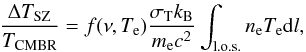$\frac{\mathrm{\Delta }{\mathit{T}}_{\mathrm{SZ}}}{{\mathit{T}}_{\mathrm{CMBR}}}\mathrm{=}\mathit{f}\mathrm{\left(}\mathit{\nu ,}{\mathit{T}}_{\mathrm{e}}\mathrm{\right)}\frac{{\mathit{\sigma }}_{\mathrm{T}}{\mathit{k}}_{\mathrm{B}}}{{\mathit{m}}_{\mathrm{e}}{\mathit{c}}^{\mathrm{2}}}{\mathrm{\int }}_{\mathrm{l}\mathit{.}\mathrm{o}\mathit{.}\mathrm{s}\mathit{.}}{\mathit{n}}_{\mathrm{e}}{\mathit{T}}_{\mathrm{e}}\mathrm{d}\mathit{l,}$(6)where T_e is the temperature of the intra-cluster medium, k_B the Boltzmann constant, T_CMBR = 2.728   °K is the temperature of the CMBR, σ_T the Thompson cross section, m_e the electron mass and f(ν,T_e) accounts for frequency shift and relativistic corrections (Itoh et al. 1998; Nozawa et al. 1998).

Other important physical phenomena occurring in the intra-galaxy cluster medium are the X-ray emission caused by thermal bremsstrahlung and line radiation resulting from electron-ion collisions. The X-ray surface brightness S_X is proportional to the integral along the line of sight of the square of the electron density. This quantity may be written as follows 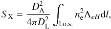${\mathit{S}}_{\mathrm{X}}\mathrm{=}\frac{{\mathit{D}}_{\mathrm{A}}^{\mathrm{2}}}{\mathrm{4}\mathit{\pi }{\mathit{D}}_{\mathrm{L}}^{\mathrm{2}}}{\mathrm{\int }}_{\mathrm{l}\mathit{.}\mathrm{o}\mathit{.}\mathrm{s}\mathit{.}}{\mathit{n}}_{\mathrm{e}}^{\mathrm{2}}{\mathrm{\Lambda }}_{\mathit{eH}}\mathrm{d}\mathit{l,}$(7)where Λ_eH is the X-ray cooling function of the intra-cluster medium (measured in the cluster rest frame) and n_e is the electron number density. It thus follows that the SZE and X-ray emission both depend on the properties (n_e, T_e) of the intra cluster medium.

As is well known, it is possible to obtain the angular diameter distance from galaxy clusters by their SZE and X-ray surface brightness observations. The calculation begins by constructing a model for the cluster gas distribution. Assuming, for instance, the spherical isothermal β-model such that n_e is given by (Cavaliere & Fusco-Fermiano 1978) 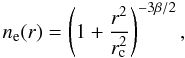${\mathit{n}}_{\mathrm{e}}\mathrm{\left(}\mathit{r}\mathrm{\right)}\mathrm{=}{\left(\mathrm{1}\mathrm{+}\frac{{\mathit{r}}^{\mathrm{2}}}{{\mathit{r}}_{\mathrm{c}}^{\mathrm{2}}}\right)}^{\mathrm{-}\mathrm{3}\mathit{\beta }\mathit{/}\mathrm{2}}\mathit{,}$(8)Eqs. (6) and (7) can be integrated. Here r_c is the core radius of the galaxy cluster. This β model is based on the hydrostatic equilibrium equation and constant temperature (Sarazin 1988). In this way, we may write for the SZE 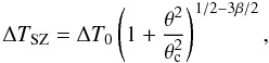$\mathrm{\Delta }{\mathit{T}}_{\mathrm{SZ}}\mathrm{=}\mathrm{\Delta }{\mathit{T}}_{\mathrm{0}}{\left(\mathrm{1}\mathrm{+}\frac{{\mathit{\theta }}^{\mathrm{2}}}{{\mathit{\theta }}_{\mathrm{c}}^{\mathrm{2}}}\right)}^{\mathrm{1}\mathit{/}\mathrm{2}\mathrm{-}\mathrm{3}\mathit{\beta }\mathit{/}\mathrm{2}}\mathit{,}$(9)where θ_c = r_c/D_A is the angular core radius and ΔT₀ is the central temperature decrement that includes all physical constants and terms resulting from the line-of-sight integration. More precisely: $\mathrm{\Delta }{\mathit{T}}_{\mathrm{0}}\mathrm{\equiv }{\mathit{T}}_{\mathrm{CMBR}}\mathit{f}\mathrm{\left(}\mathit{\nu ,}{\mathit{T}}_{\mathrm{e}}\mathrm{\right)}\frac{{\mathit{\sigma }}_{\mathrm{T}}{\mathit{k}}_{\mathrm{B}}{\mathit{T}}_{\mathrm{e}}}{{\mathit{m}}_{\mathrm{e}}{\mathit{c}}^{\mathrm{2}}}{\mathit{n}}_{\mathit{e}\mathrm{0}}\sqrt{\mathit{\pi }}{\mathit{\theta }}_{\mathrm{c}}{\mathit{D}}_{\mathrm{A}}\mathit{g}\left(\mathit{\beta }\mathit{/}\mathrm{2}\right)\mathit{,}$(10)with $\mathit{g}\mathrm{\left(}\mathit{\alpha }\mathrm{\right)}\mathrm{\equiv }\frac{\mathrm{\Gamma }\left[\mathrm{3}\mathit{\alpha }\mathrm{-}\mathrm{1}\mathit{/}\mathrm{2}\right]}{\mathrm{\Gamma }\left[\mathrm{3}\mathit{\alpha }\right]}\mathit{,}$(11)where Γ(α) is the gamma function and the others constants are the usual physical quantities. For X-ray surface brightness, we have ${\mathit{S}}_{\mathrm{X}}\mathrm{=}{\mathit{S}}_{\mathrm{X}\mathrm{0}}{\left(\mathrm{1}\mathrm{+}\frac{\mathit{\theta }}{{\mathit{\theta }}_{\mathrm{c}}^{\mathrm{2}}}\right)}^{\mathrm{1}\mathit{/}\mathrm{2}\mathrm{-}\mathrm{3}\mathit{\beta }}\mathit{,}$(12)where the central surface brightness S_X0 reads ${\mathit{S}}_{\mathrm{X}\mathrm{0}}\mathrm{\equiv }\frac{{\mathit{D}}_{\mathrm{A}}^{\mathrm{2}}{\mathrm{\Lambda }}_{\mathit{eH}}{\mathit{\mu }}_{\mathrm{e}}\mathit{/}{\mathit{\mu }}_{\mathrm{H}}}{{\mathit{D}}_{\mathrm{L}}^{\mathrm{2}}\mathrm{4}\sqrt{\mathit{\pi }}}{\mathit{n}}_{\mathit{e}\mathrm{0}}^{\mathrm{2}}{\mathit{\theta }}_{\mathrm{c}}{\mathit{D}}_{\mathrm{A}}\mathit{g}\mathrm{\left(}\mathit{\beta }\mathrm{\right)}\mathit{.}$(13)Here μ is the molecular weight given by μ_i ≡ ρ/n_im_p.

One can solve Eqs. (10) and (13) for the angular diameter distance by eliminating n_e0 and taking for granted the validity of DD relation. However, a more general result appears when the DD relation is not regarded as being strictly valid. In this case one obtains $\begin{array}{ccc}{\mathit{D}}_{\mathrm{A}}& \mathrm{=}& \left[\frac{\mathrm{\Delta }{{\mathit{T}}_{\mathrm{0}}}^{\mathrm{2}}}{{\mathit{S}}_{\mathrm{X}\mathrm{0}}}{\left(\frac{{\mathit{m}}_{\mathrm{e}}{\mathit{c}}^{\mathrm{2}}}{{\mathit{k}}_{\mathrm{B}}{\mathit{T}}_{\mathit{e}\mathrm{0}}}\right)}^{\mathrm{2}}\frac{\mathit{g}\left(\mathit{\beta }\right)}{\mathit{g}\mathrm{(}\mathit{\beta }\mathit{/}\mathrm{2}{\mathrm{)}}^{\mathrm{2}}{\mathit{\theta }}_{\mathrm{c}}}\right]\\ & & \mathrm{\times }\left[\frac{{\mathrm{\Lambda }}_{\mathit{eH}\mathrm{0}}{\mathit{\mu }}_{\mathrm{e}}\mathit{/}{\mathit{\mu }}_{\mathrm{H}}}{\mathrm{4}{\mathit{\pi }}^{\mathrm{3}\mathit{/}\mathrm{2}}\mathit{f}\mathrm{(}\mathit{\nu ,}{\mathit{T}}_{\mathrm{e}}{\mathrm{)}}^{\mathrm{2}}{\mathrm{\left(}{\mathit{T}}_{\mathrm{CMBR}}\mathrm{\right)}}^{\mathrm{2}}{{\mathit{\sigma }}_{\mathrm{T}}}^{\mathrm{2}}\mathrm{(}\mathrm{1}\mathrm{+}{\mathit{z}}_{\mathrm{c}}{\mathrm{)}}^{\mathrm{4}}}\frac{\mathrm{1}}{\mathit{\eta }\mathrm{(}\mathit{z}{\mathrm{)}}^{\mathrm{2}}}\right]\\ & \mathrm{=}& {\mathit{D}}_{\mathrm{A}}^{\mathrm{data}}{\mathit{\eta }}^{-2}\mathit{,}\end{array}$(14)where z_c is the galaxy cluster redshift. Therefore, as previously stressed by Uzan et al. (2004), galaxy cluster observations do not provide the angular diameter distance directly. In principle, instead of the real angular diameter distance, the measured quantity is ${\mathit{D}}_{\mathrm{A}}^{\mathrm{data}}\mathrm{\left(}\mathit{z}\mathrm{\right)}\mathrm{=}{\mathit{D}}_{\mathrm{A}}\mathrm{\left(}\mathit{z}\mathrm{\right)}{\mathit{\eta }}^{\mathrm{2}}\mathrm{\left(}\mathit{z}\mathrm{\right)}$.

To proceed with our analysis, the quantity η(z) defining the deformed DD relation (see Eq. (3)) is parametrically described by two different expressions (Holanda et al. 2010, 2011) $\mathit{i}\mathrm{)}\hspace{0.17em}\hspace{0.17em}\hspace{0.17em}\mathit{\eta }\mathrm{(}\mathit{z}\mathrm{)}\mathrm{=}\mathrm{1}\mathrm{+}{\mathit{\eta }}_{\mathrm{0}}\mathit{z,}\hspace{0.17em}\hspace{0.17em}\hspace{0.17em}\hspace{0.17em}\hspace{0.17em}\hspace{0.17em}\mathit{ii}\mathrm{)}\hspace{0.17em}\hspace{0.17em}\hspace{0.17em}\mathit{\eta }\mathrm{\left(}\mathit{z}\mathrm{\right)}\mathrm{=}\mathrm{1}\mathrm{+}{\mathit{\eta }}_{\mathrm{0}}\mathit{z}\mathit{/}\mathrm{(}\mathrm{1}\mathrm{+}\mathit{z}\mathrm{)}\mathit{.}$(15)The first expression is a continuous and smooth one-parameter linear expansion, whereas the second one includes a possible epoch-dependent correction that avoids the divergence at extremely high z. Naturally, one may argue that these relations were not derived from first principles. However, we stress that these expressions are very simple and have several advantages such as a manageable one-dimensional phase space and a good sensitivity to observational data. Clearly, the second parametrization can also be rewritten as η(z) = 1 + η₀(1 − a), where a(z) = (1 + z)^-1 is the cosmic-scale factor. It represents an improvement with respect to the linear parametrization, since the DD relation becomes bounded regardless of the redshift values. Potentially, it will become more useful once higher redshift cluster data are made available.

The above parametrizations are clearly inspired by similar expressions for the ω(z)-equation of state parameter in time-varying dark energy models (see, for instance, Padmanabhan & Choudury 2003; Linder 2003; Cunha et al. 2007; Silva et al. 2007). In the limit of very low redshifts (z ≪ 1), we have η = 1 and D_L = D_A as should be expected, and, more important for our subsequent analysis, the value η₀ = 0 must be favored by the Etherington principle. In other words, for a given data set, the likelihood of η₀ must be peaked at η₀ = 0, in order to satisfy the Etherington theorem. It should be remarked that Gonçalves et al. (2012) also adopted these expressions to explored the DD relation by using observations of gas mass fractions of galaxy clusters, whereas Lima et al. (2011) showed how to derive them from first principles based on possible theoretical modifications of the luminosity distance (without refraction effects).

3. Galaxy cluster samples

Fig. 1 (Color online) a) Filled (blue) circles and open (black) squares with the associated error bars (only statistical errors) stand for the De Filippis et al. (2005) samples: isothermal elliptical β model and isothermal spherical β model, respectively. b) The sample of Bonamente et al. (2006) where a non-isothermal spherical β model was used to describe the galaxy clusters.

Below, the physical constraints encoded in the possibility of a deformed DD relation is explored by considering three samples of angular diameter distances from galaxy clusters obtained by combining their SZE and X-ray surface brightness observations. The first is defined by 38 angular diameter distances from galaxy clusters in the redshift range 0.14 ≤ z ≤ 0.89, as given in the Bonamente et al. (2006) sample, where the hydrostatic equilibrium model and spherical symmetry was considered to describe the galaxy clusters. In order to construct a realistic model for the cluster gas distribution and include the possible presence of the cooling flow, these authors modeled the gas density with a function whose form is given below (Bonamente et al. 2006; La Roque et al. 2006), $\begin{array}{ccc}{\mathit{n}}_{\mathrm{e}}\mathrm{\left(}\mathit{r}\mathrm{\right)}\mathrm{=}{\mathit{n}}_{\mathit{e}\mathrm{0}}\mathrm{·}& & \left[\mathit{f}{\left(\mathrm{1}\mathrm{+}\frac{{\mathit{r}}^{\mathrm{2}}}{{\mathit{r}}_{\mathrm{c}\mathrm{1}}^{\mathrm{2}}}\right)}^{\mathrm{-}\frac{\mathrm{3}\mathit{\beta }}{\mathrm{2}}}\mathrm{+}\mathrm{(}\mathrm{1}\mathrm{-}\mathit{f}\mathrm{)}{\left(\mathrm{1}\mathrm{+}\frac{{\mathit{r}}^{\mathrm{2}}}{{\mathit{r}}_{\mathrm{c}\mathrm{2}}^{\mathrm{2}}}\right)}^{\mathrm{-}\frac{\mathrm{3}\mathit{\beta }}{\mathrm{2}}}\right]\mathit{.}\end{array}$(16)This double β-model for the density generalizes the single β-model profile, introduced by Cavaliere & Fusco-Fermiano (1976) and the double β model proposed by Mohr et al. (1999). It has the freedom of following both the central spike in density and the more gentle outer distribution. The quantity n_e0 is the central density, f governs the fractional contributions of the narrow and broad components (0 ≤ f ≤ 1), r_c1 and r_c2 are the two core radii that describe the shape of the inner and outer portions of the density distribution and β determines the slope at large radii (the same β is used for both the central and outer distributions in order to reduce the total number of degrees of freedom).

On the other hand, the hydrostatic equilibrium and spherical symmetry hypotheses result in the condition $\frac{\mathrm{d}\mathit{P}}{\mathrm{d}\mathit{r}}\mathrm{=}\mathrm{-}{\mathit{\rho }}_{\mathrm{g}}\frac{\mathrm{d}\mathit{\phi }}{\mathrm{d}\mathit{r}}\mathit{,}$(17)where P is the gas pressure, ρ_g is the gas density and φ =  −GM(r)/r is the gravitational potential due to dark matter and the plasma. Using the ideal gas equation of state for the diffuse intracluster plasma, P = ρ_gk_BT/μm_p, where μ is the mean molecular weight and m_p is the proton mass, one obtains a relationship between the cluster temperature and the cluster mass distribution, $\begin{array}{ccc}\frac{\mathrm{d}\mathit{T}}{\mathrm{d}\mathit{r}}& \mathrm{=}& \mathrm{-}\left(\frac{\mathit{\mu }{\mathit{m}}_{\mathrm{p}}}{{\mathit{k}}_{\mathrm{B}}}\frac{\mathrm{d}\mathit{\phi }}{\mathrm{d}\mathit{r}}\mathrm{+}\frac{\mathit{T}}{{\mathit{\rho }}_{\mathrm{g}}}\frac{\mathrm{d}{\mathit{\rho }}_{\mathrm{g}}}{\mathrm{d}\mathit{r}}\right)\mathit{,}\\ & \mathrm{=}& \mathrm{-}\left(\frac{\mathit{\mu }{\mathit{m}}_{\mathrm{p}}}{{\mathit{k}}_{\mathrm{B}}}\frac{\mathit{GM}}{{\mathit{r}}^{\mathrm{2}}}\mathrm{+}\frac{\mathit{T}}{{\mathit{\rho }}_{\mathrm{g}}}\frac{\mathrm{d}{\mathit{\rho }}_{\mathrm{g}}}{\mathrm{d}\mathit{r}}\right)\mathrm{·}\end{array}$(18)Bonamente et al. (2006) combined hydrostatic equilibrium equations with a dark matter density distribution from Navarro, Frenk & White (1997), ${\mathit{\rho }}_{\mathrm{DM}}\mathrm{\left(}\mathit{r}\mathrm{\right)}\mathrm{=}\mathrm{𝒩}\left[\frac{\mathrm{1}}{\mathrm{(}\mathit{r}\mathit{/}{\mathit{r}}_{\mathrm{s}}\mathrm{)}\mathrm{(}\mathrm{1}\mathrm{+}\mathit{r}\mathit{/}{\mathit{r}}_{\mathrm{s}}{\mathrm{)}}^{\mathrm{2}}}\right]\mathit{,}$(19)where is a density normalization constant and r_s is a scale radius. The parameters of these equations (n_e0, f, r_c1, r_c2, β, and r_s) were obtained by calculating the joint likelihood ℒ of the X-ray and SZE data in a Markov chain Monte Carlo method (Bonamente et al. 2004). Summarizing, the cluster plasma and dark matter distributions were analyzed assuming hydrostatic equilibrium model and spherical symmetry, thereby accounting for radial variations in density, temperature and abundance.

The second sample is formed by 25 galaxy clusters in the redshift range 0.023 ≤ z ≤ 0.8 compiled by De Filippis et al. (2005). These authors re-analyzed archival X-ray data of the XMM-Newton and Chandra satellites of two samples for which combined X-ray and SZE analysis have already been reported using an isothermal spherical β-model. One of the samples, compiled previously by Reese et al. (2002), is a selection of 18 galaxy clusters distributed over the redshift interval 0.14 < z < 0.8. The other one, the sample of Mason et al. (2001), has seven clusters from the X-ray limited flux sample of Ebeling et al. (1996). In this way, De Filippis et al. (2005) used an isothermal elliptical β-model and an isothermal spherical β model to obtain D_A(z) measurements for these galaxy clusters samples. As discussed by De Filippis et al. (2005), the choice of circular rather than elliptical β model does not affect the resulting central surface brightness or Sunyaev-Zeldovich decrement, the slope β differs slightly between these models, but significantly different values for core radius are obtained. The result was that the core radius of the elliptical β-model is bigger than that of the spherical β model (see Fig. 1 in their paper). In a first approximation it was found that ${\mathit{\theta }}_{\mathrm{ell}}\mathrm{=}\frac{\mathrm{2}{\mathit{e}}_{\mathrm{proj}}}{\mathrm{1}\mathrm{+}{\mathit{e}}_{\mathrm{proj}}}{\mathit{\theta }}_{\mathrm{circ}}$, where e_proj is the axial ratio of the major to the minor axes of the projected isophotes. Since ${\mathit{D}}_{\mathrm{A}}\mathrm{\propto }{\mathit{\theta }}_{\mathrm{c}}^{-1}$, angular diameter distances obtained by using an isothermal spherical β-model are overestimated compared with those from the elliptical β-model.

For the isothermal elliptical β-model De Filippis et al. (2005) used a general triaxial morphology to describe the intra-cluster medium. They obtained $\mathrm{\Delta }{\mathit{T}}_{\mathrm{SZ}}\mathrm{=}\mathrm{\Delta }{\mathit{T}}_{\mathrm{0}}{\left[\mathrm{1}\mathrm{+}\frac{{{\mathit{\theta }}_{\mathrm{1}}}^{\mathrm{2}}\mathrm{+}{\mathrm{\left(}{\mathit{e}}_{\mathrm{proj}}\mathrm{\right)}}^{\mathrm{2}}{{\mathit{\theta }}_{\mathrm{2}}}^{\mathrm{2}}}{{\mathrm{\left(}{\mathit{\theta }}_{\mathrm{c}\mathit{,}\hspace{0.17em}\mathrm{proj}}\mathrm{\right)}}^{\mathrm{2}}}\right]}^{\mathrm{1}\mathit{/}\mathrm{2}\mathrm{-}\mathrm{3}\mathit{\beta }\mathit{/}\mathrm{2}}\mathit{,}$(20)where $\begin{array}{ccc}\mathrm{\Delta }{\mathit{T}}_{\mathrm{0}}& \mathrm{\equiv }& {\mathit{T}}_{\mathrm{CMBR}}\mathit{f}\mathrm{\left(}\mathit{\nu ,}{\mathit{T}}_{\mathrm{e}}\mathrm{\right)}\frac{{\mathit{\sigma }}_{\mathrm{T}}{\mathit{k}}_{\mathrm{B}}{\mathit{T}}_{\mathrm{e}}}{{\mathit{m}}_{\mathrm{e}}{\mathit{c}}^{\mathrm{2}}}{\mathit{n}}_{\mathit{e}\mathrm{0}}\sqrt{\mathit{\pi }}\\ & & \mathrm{\times }\frac{{\mathit{D}}_{\mathrm{A}}{\mathit{\theta }}_{\mathrm{c}\mathit{,}\hspace{0.17em}\mathrm{proj}}}{{\mathit{h}}^{\mathrm{3}\mathit{/}\mathrm{4}}}\sqrt{\frac{{\mathit{e}}_{\mathrm{1}}{\mathit{e}}_{\mathrm{2}}}{{\mathit{e}}_{\mathrm{proj}}}}\mathit{g}\left(\mathit{\beta }\mathit{/}\mathrm{2}\right)\mathit{,}\end{array}$(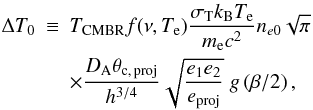21)g(α)is given by Eq. (11), D_A is the angular diameter distance to the cluster, θ_i ≡ x_i,obs/D_A is the projected angular position (on the plane of the sky) of the intrinsic orthogonal coordinate x_i,obs, h is a function of the cluster shape and orientation, e_proj is the axial ratio of the major to the minor axes of the observed projected isophotes and θ_{c,   proj} is the projection on the plane of the sky (p.o.s.) of the intrinsic angular core radius.

Similarly, the X-ray surface brightness S_X0 can be written as follows, ${\mathit{S}}_{\mathrm{X}}\mathrm{=}{\mathit{S}}_{\mathrm{X}\mathrm{0}}{\left[\mathrm{1}\mathrm{+}\frac{{{\mathit{\theta }}_{\mathrm{1}}}^{\mathrm{2}}\mathrm{+}{\mathrm{\left(}{\mathit{e}}_{\mathrm{proj}}\mathrm{\right)}}^{\mathrm{2}}{{\mathit{\theta }}_{\mathrm{2}}}^{\mathrm{2}}}{{\mathrm{\left(}{\mathit{\theta }}_{\mathrm{c}\mathit{,}\hspace{0.17em}\mathrm{proj}}\mathrm{\right)}}^{\mathrm{2}}}\right]}^{\mathrm{1}\mathit{/}\mathrm{2}\mathrm{-}\mathrm{3}\mathit{\beta }}\mathit{,}$(22)where the central surface brightness S_X0 reads ${\mathit{S}}_{\mathrm{X}\mathrm{0}}\mathrm{\equiv }\frac{{\mathrm{\Lambda }}_{\mathit{eH}}{\mathit{D}}_{\mathrm{A}}^{\mathrm{2}}\mathrm{(}{\mathit{\mu }}_{\mathrm{e}}\mathit{/}{\mathit{\mu }}_{\mathrm{H}}\mathrm{)}}{\mathrm{4}\sqrt{\mathit{\pi }}{\mathit{D}}_{\mathrm{L}}^{\mathrm{2}}}{\mathit{n}}_{\mathit{e}\mathrm{0}}^{\mathrm{2}}\frac{{\mathit{D}}_{\mathrm{A}}{\mathit{\theta }}_{\mathrm{c}\mathit{,}\hspace{0.17em}\mathrm{proj}}}{{\mathit{h}}^{\mathrm{3}\mathit{/}\mathrm{4}}}\sqrt{\frac{{\mathit{e}}_{\mathrm{1}}{\mathit{e}}_{\mathrm{2}}}{{\mathit{e}}_{\mathrm{proj}}}}\mathit{g}\mathrm{\left(}\mathit{\beta }\mathrm{\right)}\mathit{,}$(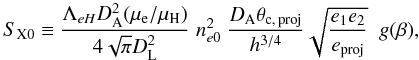23)and μ is the molecular weight, given by μ_i ≡ ρ/n_im_p.

By eliminating n_e0 in the equations above and assuming the DD relation as valid, i.e., ${\mathit{D}}_{\mathrm{A}}^{\mathrm{data}}\mathrm{\left(}\mathit{z}\mathrm{\right)}\mathrm{=}{\mathit{D}}_{\mathrm{A}}\mathrm{\left(}\mathit{z}\mathrm{\right)}$, De Filippis et al. (2005) obtained the observational quantity as written below 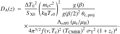$\begin{array}{ccc}{\mathit{D}}_{\mathrm{A}}\mathrm{\left(}\mathit{z}\mathrm{\right)}& \mathrm{=}& \frac{{\mathrm{\Delta }{\mathit{T}}_{\mathrm{0}}}^{\mathrm{2}}}{{\mathit{S}}_{\mathrm{X}\mathrm{0}}}{\left(\frac{{\mathit{m}}_{\mathrm{e}}{\mathit{c}}^{\mathrm{2}}}{{\mathit{k}}_{\mathrm{B}}{\mathit{T}}_{\mathit{e}\mathrm{0}}}\right)}^{\mathrm{2}}\frac{\mathit{g}\left(\mathit{\beta }\right)}{{\mathit{g}\mathrm{(}\mathit{\beta }\mathit{/}\mathrm{2}\mathrm{)}}^{\mathrm{2}}{\mathit{\theta }}_{\mathrm{c}\mathit{,}\hspace{0.17em}\mathrm{proj}}}\\ & & \mathrm{\times }\frac{{\mathrm{\Lambda }}_{\mathit{eH}\mathrm{0}}\mathrm{(}{\mathit{\mu }}_{\mathrm{e}}\mathit{/}{\mathit{\mu }}_{\mathrm{H}}\mathrm{)}}{\mathrm{4}{\mathit{\pi }}^{\mathrm{3}\mathit{/}\mathrm{2}}\mathit{f}\mathrm{(}\mathit{\nu ,}{\mathit{T}}_{\mathrm{e}}{\mathrm{)}}^{\mathrm{2}}{\mathrm{(}{\mathit{T}}_{\mathrm{CMBR}}\mathrm{)}}^{\mathrm{2}}{{\mathit{\sigma }}_{\mathrm{T}}}^{\mathrm{2}}\mathrm{(}\mathrm{1}\mathrm{+}{\mathit{z}}_{\mathrm{c}}{\mathrm{)}}^{\mathrm{4}}}\mathrm{·}\end{array}$(24)The slope β of the profile and the projected core radius θ_{c,   proj} were obtained by fitting the cluster surface brightness with an elliptical 2-D β model. For the isothermal spherical β model description, De Filippis et al. (2005) considered the usual Eq. (8) and obtained angular distances with Eq. (14) and η = 1.

In Fig. 1 we plot the galaxy cluster samples. In Fig. 1a the filled circles (blue) and open squares (black) with the associated error bars (only statistical errors) stand for the De Filippis et al. (2005) isothermal elliptical β model and isothermal spherical β model, respectively. In Fig. 1b we show the sample of Bonamente et al. (2006), where a non-isothermal spherical double β model was used to describe the galaxy clusters (red filled squares).

4. Obtaining the shape of galaxy clusters by using the DD relation as constraint

Many studies about the intra-cluster gas and dark matter (DM) distribution in galaxy clusters have been limited to the standard spherical geometry (Reiprich & Boringer 2002; Bonamente et al. 2006; Shang et al. 2009). However, in the past few years observations of galaxy clusters based on Chandra and XMM data have shown that generally clusters exhibit elliptical surface brightness maps. Simulations have also predicted that DM halos show axis ratios typically on the order of  ≈ 0.8 (Wang & White 2009), thereby disproving the spherical geometry assumption. In this line, the first determination of the intrinsic three-dimensional (3D) shapes of galaxy clusters was presented by Morandi et al. (2010) by combining X-ray, weak-lensing and strong-lensing observations. Their methodology was applied to the galaxy cluster MACS J1423.8+2404 and they found a triaxial galaxy cluster geometry with DM halo axial ratios 1.53 ± 0.15 and 1.44 ± 0.07 on the plane of the sky and along the line of sight, respectively.

Bearing in mind these results, we propose a new method to access the galaxy cluster morphology by taking the validity of the DD relation as a constraint. The idea is very simple. Beacuse the samples shown in 3 were compiled under different geometric assumptions, we confront these underlying hypotheses with the validity of the DD relation. In principle, this kind of result provides an interesting example of how a cosmological (global) condition correlates to the local physics. In the application, one should also keep in mind that a deformed DD relation as given by Eq. (3) naturally induces a more general result for the angular diameter distance from galaxy clusters via SZE and X-ray technique (see Eq. (14)) 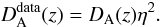${\mathit{D}}_{\mathrm{A}}^{\mathrm{data}}\mathrm{\left(}\mathit{z}\mathrm{\right)}\mathrm{=}{\mathit{D}}_{\mathrm{A}}\mathrm{\left(}\mathit{z}\mathrm{\right)}{\mathit{\eta }}^{\mathrm{2}}\mathit{.}$(25)In this line, our aim is to estimate the η₀ parameter for each galaxy cluster sample for both parameterizations of η(z) as given by Eq. (15). In our analyses (Holanda et al. 2011), D_A(z) for each galaxy clusters is obtained from the WMAP (seven years) results by fixing the conventional flat ΛCDM model. The parameters of the simplest six-parameter ΛCDM model were recently determined by Komatsu et al. (2011) by using the combination of seven-year data from WMAP with the latest distance measurements from baryon acoustic oscillations (BAO) in the distribution of galaxies (Percival et al. 2010) and the Hubble parameter H₀ measurement presented by Riess et al. (2009). The basic results are Ω_Λ = 0.725 ± 0.016 and h = 0.702 ± 0.014, and no convincing evidence for deviations from the minimal cosmic concordance model has been established.

The theoretical angular diameter distance can be written as (Lima et al. 2003; Cunha et al. 2007) 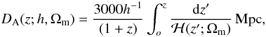${\mathit{D}}_{\mathrm{A}}\mathrm{\left(}\mathit{z}\mathrm{;}\mathit{h,}{\mathrm{\Omega }}_{\mathrm{m}}\mathrm{\right)}\mathrm{=}\frac{\mathrm{3000}{\mathit{h}}^{-1}}{\mathrm{(}\mathrm{1}\mathrm{+}\mathit{z}\mathrm{)}}{\mathrm{\int }}_{\mathit{o}}^{\mathit{z}}\frac{\mathrm{d}{\mathit{z}}^{\mathrm{\prime }}}{\mathrm{\mathscr{H}}\mathrm{\left(}{\mathit{z}}^{\mathrm{\prime }}\mathrm{;}{\mathrm{\Omega }}_{\mathrm{m}}\mathrm{\right)}}\hspace{0.17em}\mathrm{Mpc}\mathit{,}$(26)where h = H₀/100 km s^-1 Mpc^-1 and the dimensionless function ℋ(z′;Ω_m) is given by $\mathrm{\mathscr{H}}\mathrm{=}{\mathrm{\left[}{\mathrm{\Omega }}_{\mathrm{m}}\mathrm{\right(}\mathrm{1}\mathrm{+}{\mathit{z}}^{\mathrm{\prime }}{\mathrm{)}}^{\mathrm{3}}\mathrm{+}\mathrm{(}\mathrm{1}\mathrm{-}{\mathrm{\Omega }}_{\mathrm{m}}{\mathrm{\left)}}^{\mathrm{\right]}}}^{\mathrm{1}\mathit{/}\mathrm{2}}\mathit{.}$(27)Now, in order to constrain η₀, let us evaluate the likelihood distribution function, e ^− χ2/2, where ${\mathit{\chi }}^{\mathrm{2}}\mathrm{=}\sum _{\mathit{z}}\frac{{\mathrm{\{}{\mathrm{\left[}\mathit{\eta }\mathrm{\right(}\mathit{z}\mathrm{\left)}\mathrm{\right]}}^{\mathrm{2}}\mathrm{-}{\mathrm{\left[}{\mathit{\eta }}_{\mathrm{obs}}\mathrm{\right(}\mathit{z}\mathrm{\left)}\mathrm{\right]}}^{\mathrm{2}}\mathrm{\}}}^{\mathrm{2}}}{{\mathit{\sigma }}_{{\mathit{\eta }}_{\mathrm{obs}}}^{\mathrm{2}}}\mathit{,}$(28)with $\mathrm{\left[}{\mathit{\eta }}_{\mathrm{obs}}^{\mathrm{2}}\mathrm{\right(}\mathit{z}\mathrm{\left)}\mathrm{\right]}\mathrm{=}{\mathit{D}}_{\mathrm{A}}^{\mathrm{data}}\mathrm{\left(}\mathit{z}\mathrm{\right)}\mathit{/}{\mathit{D}}_{\mathrm{A}}\mathrm{\left(}\mathit{z}\mathrm{\right)}$ and ${\mathit{\sigma }}_{{\mathit{\eta }}_{\mathrm{obs}}}^{\mathrm{2}}\mathrm{=}{\left[\frac{\mathrm{1}}{{\mathit{D}}_{\mathrm{A}}\mathrm{\left(}\mathit{z}\mathrm{\right)}}\right]}^{\mathrm{2}}{\mathit{\sigma }}_{\mathrm{data}}^{\mathrm{2}}\mathrm{+}{\left[\frac{{\mathit{D}}_{\mathrm{A}}^{\mathrm{data}}}{{\mathit{D}}_{\mathrm{A}}^{\mathrm{2}}\mathrm{\left(}\mathit{z}\mathrm{\right)}}\right]}^{\mathrm{2}}{\mathit{\sigma }}_{\mathrm{WMAP}}^{\mathrm{2}}\mathit{,}$(29)where ${\mathit{\sigma }}_{\mathrm{WMAP}}^{\mathrm{2}}$ is the error in D_A(z) associated to cosmological parameters. The common statistical error contributions for galaxy clusters are SZE point sources  ± 8%, X-ray background  ± 2%, Galactic N_H ≤  ± 1%,  ± 15% for cluster asphericity,  ± 8% kinetic SZ and for CMBR anisotropy  ≤  ± 2%. On the other hand, the estimates for systematic effects are SZ calibration  ± 8%, X-ray flux calibration  ± 5%, radio halos  + 3%, and X-ray temperature calibration  ± 7.5%. Indeed, one may show that typical statistical errors amount to nearly 20%, in agreement with other works (Mason et al. 2001; Reese et al. 2002, 2004), while for systematics we also find typical errors around +12.4% and –12% (see also Table 3 in Bonamente et al. 2006). In the present analysis we have combined the statistical and systematic errors in quadrature for the galaxy clusters (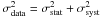${\mathit{\sigma }}_{\mathrm{data}}^{\mathrm{2}}\mathrm{=}{\mathit{\sigma }}_{\mathrm{stat}}^{\mathrm{2}}\mathrm{+}{\mathit{\sigma }}_{\mathrm{syst}}^{\mathrm{2}}$). We note that in our χ² statistical analysis the asymmetric uncertainties present in the Bonamente et al. (2006) and De Filippis et al. (2005) samples were symmetrized by using the D’Agostini (2004) method.

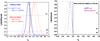Fig. 2 (Color online) a) Likelihood distribution functions for De Filippis et al. (2005) sample. The solid and the dotted blue lines are likelihood functions corresponding to linear and non-linear η(z) parametrizations for the isothermal elliptical β model. The dashed and the dashed-dotted red lines are likelihood functions corresponding to linear and non-linear parametrizations for the isothermal spherical β model. b) The likelihood distribution functions for Bonamente et al. (2006) sample. The solid blue line and the dotted red line correspond to linear and non-linear parametrizations.

In Figs. 2a and b we plot the likelihood distribution function for the De Filippis et al. (2005) and Bonamente et al. (2006) samples. The η₀ values and their errors (statistical + systematic errors) of our analysis are given below (see Table 1).

For an isothermal elliptical β model, we see that the angular diameter distances from the De Filippis et al. (2005) sample provide an excellent fit and agree with the DD relation at 1σ confidence level. On the other hand, although it agrees with the DD relation at 2σ c.l., the analysis based on the isothermal spherical β model leads to η₀ values higher than those from the elliptical β case. Since in this case η₀ > 0, the departures of the DD relation validity indicates that the estimated angular distances with the spherical β model are overestimated with respect to those from the conventional flat ΛCDM (WMAP7). For the Bonamente et al. (2006) sample (non-isothermal spherical double β model) we also see that the strict validity of the reciprocity relation is only marginally compatible. The relative situation is not modified even when only clusters with z > 0.1 are considered in the De Filippis et al. (2005) sample. In such a situation, we obtain ${\mathit{\eta }}_{\mathrm{0}}\mathrm{=}\mathrm{-}\mathrm{0.04}{\mathrm{4}}_{-0.1}^{\mathrm{+}\mathrm{0.1}}$ (χ²/d.o.f. = 15.9/17) for the linear parametrization, and ${\mathit{\eta }}_{\mathrm{0}}\mathrm{=}\mathrm{-}\mathrm{0.0}{\mathrm{7}}_{-0.14}^{\mathrm{+}\mathrm{0.14}}$ (χ²/d.o.f. = 15.6/17) within 1σ in the non-linear case for elliptical description and ${\mathit{\eta }}_{\mathrm{0}}\mathrm{=}\mathrm{0.18}{\mathrm{6}}_{-0.1}^{\mathrm{+}\mathrm{0.11}}$ (χ²/d.o.f. = 10.9/17) for the linear parametrization, and ${\mathit{\eta }}_{\mathrm{0}}\mathrm{=}\mathrm{0.27}{\mathrm{4}}_{-0.145}^{\mathrm{+}\mathrm{0.145}}$ (χ²/d.o.f. = 10.7/17) within 1σ in the non-linear case for spherical description.

Therefore, we found no evidence for a distance-duality violation for the elliptical De Filippis et al. (2005) sample. However, the same kind of analysis contradicts the spherical symmetry hypothesis assumed in the Bonamente et al. (2006) sample and in the De Filippis et al. (2005) sample when a spherical geometry is assumed. These results are very interesting since they show how important the choice of geometry is in describing the clusters to obtain their distances through SZE + X-ray measurements. We also see that the non-isothermal assumption of Bonamente et al. (2006) in their spherical description was not sufficient to satisfy the validity of the DD relation in the ΛCDM framework (WMAP7, Komatsu et al. 2011).

We recall that Bonamente et al. (2006) used three different models to describe the same 38 galaxy clusters: (i) the non-isothermal spherical double β model already discussed; (ii) an isothermal spherical β model; and (iii) the isothermal spherical β model excluding the central 100 kpc from the X-ray data. For the sake of completeness, we also obtained the η₀ values for the last two descriptions. For an isothermal spherical β model with linear and non-linear parametrizations we found ${\mathit{\eta }}_{\mathrm{0}}\mathrm{=}\mathrm{-}\mathrm{0.0}{\mathrm{9}}_{-0.06}^{\mathrm{+}\mathrm{0.05}}$ (χ²/d.o.f. = 48.48/37) and ${\mathit{\eta }}_{\mathrm{0}}\mathrm{=}\mathrm{-}\mathrm{0.1}{\mathrm{3}}_{-0.09}^{\mathrm{+}\mathrm{0.08}}$ (χ²/d.o.f. = 47.56/37), respectively. In the isothermal spherical β model excluding the central 100 kpc from the X-ray data we obtained ${\mathit{\eta }}_{\mathrm{0}}\mathrm{=}\mathrm{-}\mathrm{0.1}{\mathrm{4}}_{-0.07}^{\mathrm{+}\mathrm{0.07}}$ (χ²/d.o.f. = 47.81/37) for the linear parametrization, and ${\mathit{\eta }}_{\mathrm{0}}\mathrm{=}\mathrm{-}\mathrm{0.}{\mathrm{2}}_{-0.11}^{\mathrm{+}\mathrm{0.09}}$ (χ²/d.o.f. = 48.40/37) in the non-linear case. All these determinations are at a 1σ confidence level.

Furthermore, Bonamente et al. (2006) also determined the Hubble constant H₀ for each model. By assuming a flat ΛCDM model (Ω_M = 0.3 and Ω_Λ = 0.7), the corresponding values at 1σ c.l. are ${\mathit{H}}_{\mathrm{0}}\mathrm{=}\mathrm{76.}{\mathrm{9}}_{-3.4}^{\mathrm{+}\mathrm{3.9}}$, ${\mathit{H}}_{\mathrm{0}}\mathrm{=}\mathrm{73.}{\mathrm{7}}_{-3.8}^{\mathrm{+}\mathrm{4.6}}$ and ${\mathit{H}}_{\mathrm{0}}\mathrm{=}\mathrm{77.}{\mathrm{6}}_{-4.3}^{\mathrm{+}\mathrm{4.8}}$. More recently, Cunha et al. (2007) obtained H₀ = 74 ± 3.5 through a joint analysis with BAO by using the De Filippis et al. sample (2005), thereby alleviating the tension between between SZ + X-ray technique and the CMB + BAO determination of H₀. However, since the Hubble constants obtained from all these models agree at 1σ, one may conclude that the H₀ value is not useful to decide which galaxy cluster model is more realistic.

5. Testing the DD relation with galaxy clusters and SNe Ia

In this section we apply a model-independent cosmological test for the DD relation based on the three samples defined in Sect. 3. For D_L we considered two subsamples of SNe type Ia taken from Tables 1 and 2 of the Hicken et al. (2009) (Constitution data), whereas values for D_A are provided by the three samples of galaxy clusters discussed above. The SNe Ia redshifts of each subsample were carefully chosen to coincide with those of the associated galaxy cluster sample (Δz < 0.005), thereby allowing a direct test of the DD relation. For a given pair of data sets (SNe Ia, galaxy clusters), one should expect a likelihood of η₀ peaked at η₀ = 0, in order to satisfy the DD relation. Moreover, in our approach the data do not need to be binned as assumed in some analyses involving the DD relation (see, for instance, De Bernardis et al. 2006).

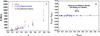Fig. 3 (Color online) a) Galaxy clusters and SNe Ia data. The open blue, open black, and filled red circles with the associated error bars stand for the galaxy clusters described with elliptical and spherical β models of the De Filippis et al. (2005) (statistical + systematical errors) and SNe Ia (only statistical errors) samples, respectively. b) The redshift subtraction for the same pair of cluster-SNe Ia samples. The open squares represent the pairs of points for which Δz ≈ 0.01.

In Fig. 3a we plot D_A multiplied by (1 + z_cluster)² from the galaxy clusters sample compiled from the De Filippis et al. (2005) sample and D_L from our first SNe Ia subsample. In Fig. 3b we plot the subtraction of redshift between clusters and SNe Ia. We see that the biggest difference is Δz ≈ 0.01 for three clusters (open squares), while for the remaining 22 clusters we have Δz < 0.005. In order to avoid the corresponding bias, we removed the three clusters from all subsequent analyses so that Δz < 0.005 for all pairs.

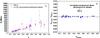Fig. 4 (Color online) a) Galaxy clusters and SNe Ia data. The open (blue) and filled (red) circles with the associated error bars stand for the Bonamente et al. (2006) (statistical + systematical errors) and SNe Ia (only statistical errors) samples, respectively. b) The redshift subtraction for the same pair of cluster-SNe Ia samples. As in Fig. 1b, the open squares represent the pairs of points with the biggest difference in redshifts (Δz ≈ 0.01).

Similarly, in Fig. 4a we plot D_A multiplied by (1 + z_cluster)², but now for the Bonamente et al. sample (2006) and D_L from our second SNe Ia subsample. In Fig. 4b we display the redshift subtraction between clusters and SNe Ia. Again, we see that for 35 clusters Δz < 0.005. The biggest difference is again Δz ≈ 0.01 for three clusters, and, for consistency, these were also removed from our analysis.

Let us now estimate the parameter η₀ for each sample and the two parametrizations defined by Eq. (3). We recall that in general the SZE + X-ray surface brightness observations technique does not produce D_A(z), but 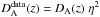${\mathit{D}}_{\mathrm{A}}^{\mathrm{data}}\mathrm{\left(}\mathit{z}\mathrm{\right)}\mathrm{=}{\mathit{D}}_{\mathrm{A}}\mathrm{\left(}\mathit{z}\mathrm{\right)}{\mathit{\eta }}^{\mathrm{2}}$. Consequently, if one wishes to test Eq. (1) with SZE + X-ray observations from galaxy clusters, the angular diameter distance must be replaced by ${\mathit{D}}_{\mathrm{A}}^{\mathrm{data}}\mathrm{\left(}\mathit{z}\mathrm{\right)}{\mathit{\eta }}^{-2}$ in Eq. (3). In this way, we obtained $\mathit{\eta }\mathrm{\left(}\mathit{z}\mathrm{\right)}\mathrm{=}{\mathit{D}}_{\mathrm{A}}^{\mathrm{data}}\mathrm{\left(}\mathit{z}\mathrm{\right)}\mathrm{(}\mathrm{1}\mathrm{+}{\mathit{z}}_{\mathrm{cluster}}{\mathrm{)}}^{\mathrm{2}}\mathit{/}{\mathit{D}}_{\mathrm{L}}\mathrm{(}\mathit{z}\mathrm{)}$.

Following standard procedure, the likelihood estimator is determined by a χ² statistics ${\mathit{\chi }}^{\mathrm{2}}\mathrm{=}\sum _{\mathit{z}}\frac{{\left[\mathit{\eta }\mathrm{\left(}\mathit{z}\mathrm{\right)}\mathrm{-}{\mathit{\eta }}_{\mathrm{obs}}\mathrm{\left(}\mathit{z}\mathrm{\right)}\right]}^{\mathrm{2}}}{{\mathit{\sigma }}_{{\mathit{\eta }}_{\mathrm{obs}}}^{\mathrm{2}}}\mathit{,}$(30)where ${\mathit{\eta }}_{\mathrm{obs}}\mathrm{\left(}\mathit{z}\mathrm{\right)}\mathrm{=}\mathrm{(}\mathrm{1}\mathrm{+}{\mathit{z}}_{\mathrm{cluster}}{\mathrm{)}}^{\mathrm{2}}{\mathit{D}}_{\mathrm{A}}^{\mathrm{data}}\mathrm{(}\mathit{z}\mathrm{)}\mathit{/}{\mathit{D}}_{\mathrm{L}}\mathrm{(}\mathit{z}\mathrm{)}$ and $\begin{array}{ccc}{\mathit{\sigma }}_{{\mathit{\eta }}_{\mathrm{obs}}}^{\mathrm{2}}& \mathrm{=}& {\left[\frac{\mathrm{(}\mathrm{1}\mathrm{+}{\mathit{z}}_{\mathrm{cluster}}{\mathrm{)}}^{\mathrm{2}}{\mathit{D}}_{\mathrm{A}}^{\mathrm{data}}}{{\mathit{D}}_{\mathrm{L}}^{\mathrm{2}}}\right]}^{\mathrm{2}}{\mathit{\sigma }}_{{\mathit{D}}_{\mathrm{L}}}^{\mathrm{2}}\mathrm{+}{\left[\frac{\mathrm{(}\mathrm{1}\mathrm{+}{\mathit{z}}_{\mathrm{cluster}}{\mathrm{)}}^{\mathrm{2}}}{{\mathit{D}}_{\mathrm{L}}}\right]}^{\mathrm{2}}{\mathit{\sigma }}_{{\mathit{D}}_{\mathrm{A}}^{\mathrm{data}}}^{\mathrm{2}}\mathit{.}\end{array}$(31)As in the previous section, we combined the statistical and systematic errors in quadrature for the angular diameter distance from galaxy clusters, and, as we remarked above, the asymmetric error bars were treated by the D’Agostini (2004) method.

On the other hand, after nearly 500 discovered SNe Ia, the constraints on the cosmic parameters from luminosity distance are now limited by systematics rather than by statistical errors. In principle, there are two main sources of systematic uncertainties in SNe Ia observations, which are closely related to photometry and possible corrections for light-curve shape (Hicken at al. 2009). However, at the moment it is not so clear how one is to estimate the overall systematic effects for these standard candles (Komatsu et al. 2011), and, therefore, we exclude them from the following analysis. The basic reason is that systematic effects from galaxy clusters seem to be larger than those of SNe observations, but their inclusion does not affect the results validity of the distance-duality relation very much. In this way, following Holanda et al. (2010), we included only statistical errors of the SNe Ia magnitude measurements.

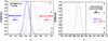Fig. 5 (Color online) a) Likelihood distribution functions for De Filippis et al. (2005) sample. The solid and the dotted blue lines are likelihood functions for linear and non-linear parametrizations corresponding to the isothermal elliptical β model. The dashed and the dashed-dotted red lines are likelihood functions for linear and non-linear parametrizations corresponding to the isothermal spherical β model. b) The likelihood distribution functions for Bonamente et al. (2006) sample.

In Figs. 5a and b we plot the likelihood distribution function for each sample. The η₀ values with their errors (statistical and systematic errors) are provided in Table 2. Clearly, the confrontation between the angular diameter distances from the elliptical De Filippis et al. (2005) sample with SNe Ia data disagree moderately with the reciprocity relation (the DD relation is marginally satisfied in 2σ) and the η₀ values are mostly negative. Since $\mathrm{(}\mathrm{1}\mathrm{+}{\mathit{z}}_{\mathrm{cluster}}{\mathrm{)}}^{\mathrm{2}}{\mathit{D}}_{\mathrm{A}}^{\mathrm{data}}\mathrm{(}\mathit{z}\mathrm{)}\mathit{/}{\mathit{D}}_{\mathrm{L}}\mathrm{(}\mathit{z}\mathrm{)}\mathrm{\propto }\mathrm{1}\mathrm{+}{\mathit{\eta }}_{\mathrm{0}}\mathit{z}$, negative η₀ values indicate luminosity distances overestimated with respect to the angular diameter ones. This tension between Sne Ia and the elliptical De Filippis et al. (2005) sample arises because SNe Ia samples prefer universes with a higher Ω_Λ value than those of the WMAP7 results. Indirectly, our analysis support the tension found by Wei (2010), who used SNe Ia constitution data and observations of the CMBR anisotropy plus BAO separately to constrain the ω_a parameter of the dark energy equation of state given by ω = ω₀+ω_az/(1 + z). The SNe Ia constitution data indicated a strong negative ω_a (ω_a ≈  −11) and the phantom energy divide line (ω <  − 1) could be crossed at recent redshifts. Furthermore, the constitution data disagreed not only with the CMB and BAO observations, but also with other SNe Ia datasets such as Davis (Davis et al. 2007) and SNLS (Astier et al. 2006). On the other hand, when an isothermal spherical β model is used, the DD relation is satisfied in 1σ. As discussed earlier, this concordance occurs because an isothermal spherical β model yields angular distances overestimated compared to the elliptical model and WMAP7 results. For the Bonamente et al. (2006) sample, where a non-isotermal spherical double β model was assumed to describe the clusters, we see that the DD relation is not obeyed even at 3σ. We note that our results do not change if one replaces z_cluster by z_SNe, where z_SNe is the redshift of SNe Ia. This shows that a Δz < 0.005 is sufficient to implement our direct test.

In this context, we recall that Li et al. (2011) rediscussed this independent cosmological test using the latest Union2 SNe Ia data and the angular diameter distances from galaxy clusters. However, they removed six and twelve data points, respectively, from the De Filippis et al. (2005) and Bonamente et al. (2006) samples and obtained a more serious violation of the DD relation. These authors also reexamined the DD relation by postulating two more general parameterization forms, namely η(z) = η₀ + η₁z and η(z) = η₀ + η₁z/(1 + z), and they found that consistencies between the observations and the DD relation are markedly improved for both samples of galaxy clusters. Nair et al. (2011) also discussed the strict validity of the DD relation using the latest Union2 SNe Ia data and the angular diameter distances from galaxy clusters, FRIIb radio galaxies and mock data. They proposed six different (one and two indices) parametrizations (including, as particular cases, those adopted by Holanda et al. 2010) in an attempt to determine a possible redshift variation of the DD relation. As physically expected, their results depend both on the specific parametrization and the data samples considered. In particular, they conclude that one index parameterization, namely η_V = η₈/(1 + z) and η_V = η₉exp {  [z/(1 + z)] /(1 + z) } , do not support the DD relation for the given data set.

More recently, Meng et al. (2012) also reinvestigated the model-independent test by comparing two different methods and several parametrizations (one and two indices) for η(z). Their basic conclusion agrees with our studies in the sense that the triaxial ellipsoidal model is suggested by the model-independent test at 1σ while the spherical β model can only be accommodated at a 3σ confidence level. As we shall see, this uncertainty can also be robustly resolved by considering a joint analysis involving the two treatments discussed here (see Sect. 7). In principle, since all results somewhat depend on the assumed η(z) form, it is important to understand the effect of different parametrizations. However, we recall that at extremely low redshifts the DD relation reduces to unity since D_L(z) ≡ D_A(z), and, therefore, the constant parameter appearing in the proposed η(z) expressions should be fixed to unity.

At this point it is interesting to know the influence of SNe Ia light-curve fitters on the model-independent test of the distance duality relation and some of its consequences for the local physics. This topic has attracted a lot of attention in the recent literature (Kessler et al. 2009; Bengochea 2011; Hao Wei 2010), and its connection with the DD relation and galaxy cluster geometry it will be discussed next.

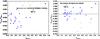Fig. 6 (Color online) a) Redshift subtraction for the same pair of cluster-SNe Ia samples of De Filippis et al. (2005). The open squares represent the pairs of points for which Δz > 0.005. b) The redshift subtraction for the same pair of cluster-SNe Ia samples for Bonamente et al. (2006). The open squares represent the pairs of points for which Δz > 0.005.

6. SNe Ia light-curve fitters, DD relation and cluster geometries

In the previous section, we tested the DD relation by using luminosity distances from SNe Ia based on the Constitution sample and the angular diameter distances from three galaxy clusters samples obtained by their SZE and X-rays surface brightness measurements. However, in the Constitution compilation different SNe Ia samples were analyzed by four light-curve fitters (SALT, SALT2, MLCS31 and MLCS17) to test consistency and systematic differences: 397 SNe Ia with SALT, 351 SNe Ia with SALT2, 366 SNe Ia with MLCS31 and 372 SNe Ia with MLCS17. The four fitters were seen to be relatively consistent with the light-curve-shape and color parameters, but that still leaves room for improvement, and they provide a considerable amount of systematic uncertainty to any analysis. In this way, it would be interesting to investigate the influence of different SNe Ia light-curve fitters on our previous results. Unfortunately, it was not possible to find the same SNe’s Ia used here in Sect. 5 in the Constitution sample, but analyzed with the four methods for a direct comparison.

On the other hand, Kessler et al. (2009) presented the Hubble diagram for 103 SNe Ia with redshifts 0.04 < z < 0.42, discovered during the first season of the Sloan Digital Sky Survey-II (SDSS-II). These data filled the redshift desert between low- and high-redshift SNe Ia of the previous SNe Ia surveys. In addition, these authors included a comprehensive and consistent reanalysis of other datasets (ESSENCE, SNLS, HST), resulting in a combined sample of 288 SNe Ia. Reanalysis was performed by using two light-curve fitters: SALT2 (Guy et al. 2007) and MLCS2K2 (Jha et al. 2007). MLCS2K2 calibration uses a nearby training set of SNe Ia assuming a close to linear Hubble law, while SALT2 uses the whole data set to calibrate empirical light curve parameters, and a cosmological model must be assumed in this method. Typically a ΛCDM or a ωCDM model is assumed. Consequently, the SNe Ia distance moduli obtained with SALT2 fitter retain a degree of model dependence (Bengochea 2011). Kessler et al. (2009) combined these 288 SNe Ia with measurements of baryon acoustic oscillations from the SDSS luminous red galaxy sample and with cosmic microwave background temperature anisotropy measurements from the WMAP for estimating the cosmological parameters ω and Ω_M by assuming a spatially flat cosmological model. The results from these two light-curve fitters disagreed: ω =  −0.76 ± 0.07(stat)  ±    0.11(syst), Ω_M = 0.307 ± 0.019 (stat)  ±    0.023(syst) using MLCS2K2 and ω =  −0.96 ± 0.06(stat)  ±    0.12(syst), Ω_M = 0.265 ± 0.016(stat)  ±    0.025(syst) using SALT2. This discrepancy raised the question of which method is more reliable because it is not possible to definitively determine from the current data that either method is better or incorrect. The overall conclusion was that the cosmological parameter ω lies between  − 1.1 and  − 0.7 (Kessler et al. 2009). Exploring nonstandard cosmology scenarios, Sollerman et al. (2009) found that more exotic models provided a better fit to the SNe Ia data than the ΛCDM model when the MLCS2K2 light-curve fitter was used. However, when the SN Ia data were analyzed by using SALT2 light-curve fitter, the standard cosmological constant model agreed better to those data.

In this section, by using the SNe Ia data from SDSS-II (Kessler et al. 2009), we explore the influence of the two different SNe Ia light-curve fitters on our model-independent cosmological test for the DD relation. For D_L we considered two subsamples of SNe Ia taken from SDSS-II (2007) where, again, the SNe Ia redshifts of each subsample were carefully chosen to coincide with those of the associated galaxy cluster sample (Δz < 0.005), allowing a direct test of the DD relation. Furthermore, in this case, each subsample of SNe Ia was analyzed by the MLCS2K2 and SALT2 light-curve fitters separately. For D_A we used the angular diameter distance samples of galaxy clusters discussed above: the isothermal elliptical and spherical β model samples from De Filippis et al. (2005) and the non-isothermal spherical double β model sample from Bonamente et al. (2006).

In Fig. 6a we plot the subtraction of redshift between clusters and SNe Ia for the De Filippis et al. (2005) sample. We see that the biggest difference is Δz ≈ 0.007 for three clusters (open squares), whereas for the remaining 22 clusters we have Δz < 0.005. In order to avoid the corresponding bias, the three clusters were removed from all analyses presented here so that Δz < 0.005 for all pairs. In Fig. 6b we display the redshift subtraction between clusters and SNe Ia for the Bonamente et al. (2006) sample. In this case we see that for 33 clusters Δz < 0.005. The biggest difference is Δz ≈ 0.015 for five clusters, and, for consistency, they were also removed from our analysis.

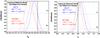Fig. 7 (Color online) a) Likelihood distribution functions for the De Filippis et al. (2005) sample (elliptical β model) for both η(z) parametrizations and both SNe Ia light-curve fitters. b) The likelihood distribution functions for the De Filippis et al. (2005) sample (spherical β model) for both η(z) parametrizations and both SNe Ia light-curve fitters.

In Figs. 7a and b we plot the likelihood distribution function for the elliptical and spherical De Filippis et al. (2005) samples, respectively. The results for Bonamente et al. (2006) sample are shown in Fig. 8. Following Kessler et al. (2009) and Sollerman et al. (2009), we added in our analyses an additional intrinsic dispersion of 0.16 mag to the uncertainties output by the MLCS2K2 light-curve fitter and 0.14 mag for the SALT2 light-curve fitter. In Table 3 we display our results, where the errors are in 2σ (statistical plus systematic errors).

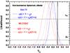Fig. 8 (Color online) a) Likelihood distribution functions for the Bonamente et al. (2006) sample for both parametrizations and both SNe Ia light-curve fitters.

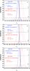Fig. 9 (Color online) a) Joint analysis for the De Filippis et al. (2005) samples and WMAP + SNe Ia (Constitution Sample). b) Joint analysis for the De Filippis et al. (2005) samples and WMAP + SNe Ia (SDSS-SALT2). c) Joint analysis for the De Filippis et al. (2005) samples and WMAP + SNe Ia (SDSS-MLCS2k2).

Interestingly, we also obtained conflicting results between the two light-curve fitters. In our analysis involving the elliptical De Filippis et al. (2005) sample (for both light-curve fitters), the DD relation validity is obtained at 1σ (c.l.) with the SALT2 method. However, it is only marginally compatible with MLC2K2 method because the η₀ values are considerably negative. This result points to an overestimated luminosity distances when SNe Ia are analyzed with the MLC2K2 method. This result is not surprising since the De Filippis et al. (2005) sample agrees with the DD relation validity in the context of the ΛCDM model (WMAP7) (see Sect. 4) and the SALT2 light-curve fitter also favors the same cosmology according to the analyses of Kessler et al. (2009) and Sollerman et al. (2009). Curiously, the best verification of the DD relation validity is obtained by confronting the spherical sample of De Filippis et al. (2005) with SNe Ia when the MLC2K2 light-curve fitter is adopted. This probably occurs because both distances are overestimated compared to distances from the elliptical model and the ΛCDM model (WMAP7). For the Bonamente et al. (2006) sample the DD relation validity is marginally compatible (2σ) with SALT2 and at 3σ with MLCS2K2.

7. Searching for the true geometry of clusters: a joint analysis

In the previous sections we have discussed how the validity of the DD relation can be used to fix the true cluster geometry by using two independent approaches: (i) the model-dependent test based on the SZE/X-ray technique in the context of the ΛCDM model (WMAP7 analysis), and (ii) the model-independent test using the combination of SZE/X-ray for galaxy clusters and SNe Ia data. For the former case the elliptical description provides the best fit supporting the standard DD relation in ΛCDM (Komatsu et al. 2011). On the other hand, the isothermal spherical β model is more compatible with the validity of the DD relation in the model-independent test involving supernovas. Since likelihoods for both descriptions in both approaches (see Figs. 2a and 5a) are compatible with each other in at least 2-sigma, it is convenient to perform a joint analysis involving these independent and complementary treatments in order to choose the better description.

Naturally, one may argue that the joint analysis will be plagued by the underlying tension between SNe and CMB data. In this context, we recall that this tension was recently discussed by taking into account weak-lensing effects caused by inhomogeneities at low and intermediate redshifts by Amendola et al. (2010). By using the Union data (2008), they showed that the inclusion of lensing moves the best-fit model significantly toward the flat LCDM model (owing to corrections induced by the lens convergence on the distance modulus). This treatment is beyond the scope of our paper. Nevertheless, this treatment is valid in the same sense as the early analysis involving SNe Ia and CMB were to the cosmic concordance model. As we shall see, the joint analysis below confirms that the elliptical isothermal model provides the best description for galaxy clusters.

Now, by adding the χ² statistics for the different approaches, the resulting likelihoods for the η₀ parameter were again obtained. The main findings for both parametrizations (linear and non-linear cases) are summarized in Table 4. Note that we restricted our attention to the De Filippis et al. (2005) samples (elliptical and spherical isothermal assumptions).

From Table 4, we see that the elliptical geometry agrees better with the strict validity of the duality relation when both approaches are considered. This result remains valid regardless of the supernova sample (Constitution or SDSS) adopted, the parameterization (linear or non-linear), or the kind of light fitter used.

In Fig. 9, we plotted the likelihoods function for the η₀ parameter as obtained from our joint analysis by considering again the De Filippis et al. (2005) samples (elliptical and spherical isothermal geometries). Figure 9a is the joint analysis for the WMAP + SNe Ia by using the Constitution sample while in Figs. 9b and c, we considered SDSS sample, but now taking into account the different light-curve fitters (SALT2 and MLCS2k2). The horizontal lines are cuts in the regions of 68.3 (1σ) per cent and 95.4 (2σ) per cent probability. Our joint analysis shows that an elliptical geometry is suggested by the existing data even when we take into account the SNe Ia light-curve fitters. Because several SZE surveys are in progress, our results call attention to a basic difficulty involving the spherical assumption to describe the cluster morphology when independent cosmological probes are considered.

8. Conclusions

We explored some physical consequences of a deformed distance-duality relation, η(z) = D_L(1 + z)^-2/D_A, based on observations of galaxy clusters using SZE and X-ray surface brightness. The η(z) parameter was described by two distinct forms, η = 1 + η₀z and η = 1 + η₀z/(1 + z), thereby recovering the standard equality between distances for extremely low redshifts.

Initially, we discussed the consistency between the strict validity of the distance-duality relation and the underlying assumptions about the galaxy cluster geometries. In our analysis we used angular diameter distances from galaxy clusters of the De Filippis et al. (2005) and Bonamente et al. (2006) samples. The former sample consists of 25 data sets where the galaxy clusters were described by an isothermal elliptical β model and a spherical β model, whereas the latter sample consists of 38 data sets where a non-isothermal spherical double β model was used. We showed that the elliptical geometry is more consistent with no violation of the distance duality relation in the context of ΛCDM (WMAP7 data). In the elliptical case of the De Filippis et al. (2005) sample (see Fig. 2a and Table 1) we found ${\mathit{\eta }}_{\mathrm{0}}\mathrm{=}\mathrm{-}\mathrm{0.05}{\mathrm{6}}_{-0.1}^{\mathrm{+}\mathrm{0.1}}$ and ${\mathit{\eta }}_{\mathrm{0}}\mathrm{=}\mathrm{-}\mathrm{0.08}{\mathrm{8}}_{-0.14}^{\mathrm{+}\mathrm{0.14}}$ for linear and non-linear parametrizations at 1σ (statistical plus systematic errors), respectively. The analysis with the isothermal spherical β model led to higher and positive η₀ values than those from elliptical β model, indicating that the estimated angular distances with the spherical β model are overestimated compared to those from ΛCDM (WMAP7). On the other hand, the non-isothermal spherical double β model (see Fig. 2b) was only marginally compatible with η₀ = 0, such as ${\mathit{\eta }}_{\mathrm{0}}\mathrm{=}\mathrm{-}\mathrm{0.1}{\mathrm{2}}_{-0.12}^{\mathrm{+}\mathrm{0.12}}$ and ${\mathit{\eta }}_{\mathrm{0}}\mathrm{=}\mathrm{-}\mathrm{0.17}{\mathrm{5}}_{-0.175}^{\mathrm{+}\mathrm{0.175}}$ for linear and non-linear parameterizations at 2σ (statistical plus systematic errors), respectively. In this way, our analysis revealed that the elliptical model is compatible with the duality relation at 1σ, whereas the non-isothermal spherical model (in Bonamente et al. 2006 sample) is only marginally compatible at 3σ in the ΛCDM framework.

Furthermore, we discussed a new and model-independent cosmological test for the distance-duality relation. We considered the three angular diameter distance samples from galaxy clusters, which are obtained by using SZE and X-ray surface brightness, together the luminosity distances given by two subsamples of SNe Ia taken from the Constitution data. For each subsample, the redshifts of the SNe Ia were carefully chosen to coincide with those of the associated galaxy cluster sample (Δz < 0.005). Our results showed that the confrontation between the angular diameter distances from the De Filippis et al. (2005) sample (elliptical model) with SNe Ia data pointed to a moderate violation of the reciprocity relation (the DD relation was marginally satisfied in 2σ) and the η₀ values were predominantly negative. Since $\mathrm{(}\mathrm{1}\mathrm{+}\mathit{z}{\mathrm{)}}^{\mathrm{2}}{\mathit{D}}_{\mathrm{A}}^{\mathrm{data}}\mathrm{(}\mathit{z}\mathrm{)}\mathit{/}{\mathit{D}}_{\mathrm{L}}\mathrm{(}\mathit{z}\mathrm{)}\mathrm{\propto }\mathrm{1}\mathrm{+}{\mathit{\eta }}_{\mathrm{0}}\mathit{z}$, negative η₀ values indicated luminosity distances overestimated with relation to angular diameter ones. This tension between Sne Ia and the elliptical De Filippis et al. (2005) sample arises because SNe Ia samples prefer universes with higher Ω_Λ values than the WMAP7 results. When an isothermal spherical β model is adopted, the DD relation had been satisfied at 1σ with η₀ values preferably positive. Seemingly, this concordance occurred only because an isothermal spherical β model yields angular distances overestimated in comparison to an elliptical model and WMAP7 results. For the Bonamente et al. (2006) sample, where a non-isotermal spherical double β model was assumed to describe the clusters, we saw that the DD relation is not obeyed even at 3σ. For this case we obtained ${\mathit{\eta }}_{\mathrm{0}}\mathrm{=}\mathrm{-}\mathrm{0.4}{\mathrm{2}}_{-0.34}^{\mathrm{+}\mathrm{0.34}}$ and ${\mathit{\eta }}_{\mathrm{0}}\mathrm{=}\mathrm{-}\mathrm{0.6}{\mathrm{6}}_{-0.5}^{\mathrm{+}\mathrm{0.5}}$ for linear and non-linear η(z) parameterizations in 3σ (statistical plus systematic errors), respectively.

Moreover, by using the SNe Ia data from SDSS-II (Kessler et al. 2009), we explored the influence of the two different SNe Ia light-curve fitters in our model-independent cosmological test for the DD relation. In this way, we considered two subsamples of SNe Ia taken from SDSS-II (2007) for D_L where, again, the SNe Ia redshifts of each subsample were carefully chosen to coincide with those of the associated galaxy cluster sample (Δz < 0.005). In this case, each subsample of SNe Ia was analyzed by the MLCS2K2 and SALT2 light-curve fitters separately. Interestingly, we obtained conflicting results between the two light-curve fitters. For both light-curve fitter-method the best fits are obtain in an analysis involving the elliptical De Filippis et al. (2005) sample. In this case, the DD relation validity was obtained in 1σ with the SALT2 method and it was marginally compatible with MLC2K2 method with η₀ values considerably negative. This result points to overestimated luminosity distances when SNe Ia are analyzed with MLC2K2 method. For this light-curve fitter, the isothermal spherical β model provided that the DD relation was satisfied at 1σ. For all tests of the Bonamente et al. (2006) sample, the DD relation validity is obtained marginally at 2σ (SALT2) and at 3σ (MLCS2K2). We stress that our results are independent of the redshifts chosen to realize the test (of the galaxy clusters or SNe Ia), thereby showing the robustness of the method and supporting Δz < 0.005 as a fair choice.

Finally, we applied a joint analysis involving these independent and complementary treatments by adding the χ² statistics for the different approaches. Interestingly, we saw that the elliptical geometry agrees better with the strict validity of the duality relation when both approaches were considered. This result remains valid regardless of the adopted SNe Ia sample (Constitution or SDSS), the parameterization (linear or non-linear), or the kind of light-curve fitter used (see Table 4). The non-isothermal spherical double β model was only marginally compatible with the DD relation validity in all treatments.

Summarizing, the statistical analysis presented here provides new evidence that the true geometry of clusters has an elliptical form. In principle, it is remarkable that a local property such as the geometry of galaxy clusters may be constrained by a global argument like the one provided by the cosmological distance-duality relation. This result also reinforces the interest in the observational search for SZE and X-ray from clusters at high redshifts. In the near future, when more and larger samples with smaller statistical and systematic uncertainties become available, the method proposed here, based on the validity of the distance-duality relation, can improve the limits on the possible cluster geometries and explore systematic errors in SNe Ia and galaxy clusters observations.

Acknowledgments

R.F.L.H. is supported by FAPESP (No. 07/52912-2) and J.A.S.L. is partially supported by CNPq (No. 306054/2010) and FAPESP (No. 04/13668-0).

References

All Tables

All Figures

	Fig. 1 (Color online) a) Filled (blue) circles and open (black) squares with the associated error bars (only statistical errors) stand for the De Filippis et al. (2005) samples: isothermal elliptical β model and isothermal spherical β model, respectively. b) The sample of Bonamente et al. (2006) where a non-isothermal spherical β model was used to describe the galaxy clusters.
In the text

Fig. 2 (Color online) a) Likelihood distribution functions for De Filippis et al. (2005) sample. The solid and the dotted blue lines are likelihood functions corresponding to linear and non-linear η(z) parametrizations for the isothermal elliptical β model. The dashed and the dashed-dotted red lines are likelihood functions corresponding to linear and non-linear parametrizations for the isothermal spherical β model. b) The likelihood distribution functions for Bonamente et al. (2006) sample. The solid blue line and the dotted red line correspond to linear and non-linear parametrizations.

In the text

Fig. 3 (Color online) a) Galaxy clusters and SNe Ia data. The open blue, open black, and filled red circles with the associated error bars stand for the galaxy clusters described with elliptical and spherical β models of the De Filippis et al. (2005) (statistical + systematical errors) and SNe Ia (only statistical errors) samples, respectively. b) The redshift subtraction for the same pair of cluster-SNe Ia samples. The open squares represent the pairs of points for which Δz ≈ 0.01.

In the text

Fig. 4 (Color online) a) Galaxy clusters and SNe Ia data. The open (blue) and filled (red) circles with the associated error bars stand for the Bonamente et al. (2006) (statistical + systematical errors) and SNe Ia (only statistical errors) samples, respectively. b) The redshift subtraction for the same pair of cluster-SNe Ia samples. As in Fig. 1b, the open squares represent the pairs of points with the biggest difference in redshifts (Δz ≈ 0.01).

In the text

Fig. 5 (Color online) a) Likelihood distribution functions for De Filippis et al. (2005) sample. The solid and the dotted blue lines are likelihood functions for linear and non-linear parametrizations corresponding to the isothermal elliptical β model. The dashed and the dashed-dotted red lines are likelihood functions for linear and non-linear parametrizations corresponding to the isothermal spherical β model. b) The likelihood distribution functions for Bonamente et al. (2006) sample.

In the text

	Fig. 6 (Color online) a) Redshift subtraction for the same pair of cluster-SNe Ia samples of De Filippis et al. (2005). The open squares represent the pairs of points for which Δz > 0.005. b) The redshift subtraction for the same pair of cluster-SNe Ia samples for Bonamente et al. (2006). The open squares represent the pairs of points for which Δz > 0.005.
In the text

	Fig. 7 (Color online) a) Likelihood distribution functions for the De Filippis et al. (2005) sample (elliptical β model) for both η(z) parametrizations and both SNe Ia light-curve fitters. b) The likelihood distribution functions for the De Filippis et al. (2005) sample (spherical β model) for both η(z) parametrizations and both SNe Ia light-curve fitters.
In the text

	Fig. 8 (Color online) a) Likelihood distribution functions for the Bonamente et al. (2006) sample for both parametrizations and both SNe Ia light-curve fitters.
In the text

	Fig. 9 (Color online) a) Joint analysis for the De Filippis et al. (2005) samples and WMAP + SNe Ia (Constitution Sample). b) Joint analysis for the De Filippis et al. (2005) samples and WMAP + SNe Ia (SDSS-SALT2). c) Joint analysis for the De Filippis et al. (2005) samples and WMAP + SNe Ia (SDSS-MLCS2k2).
In the text

References

- Albani, V. V. L., Iribarrem, A. S., Ribeiro, M. B., & Stoeger, W. R. 2007, ApJ, 657, 760 [NASA ADS] [CrossRef] [Google Scholar]
- Amanullah, R., Lidman, C., Rubin, D., et al. 2010, ApJ, 716, 712 [NASA ADS] [CrossRef] [Google Scholar]
- Astier, P., Guy, J., Regnault, N., et al. 2006, A&A, 447, 31 [NASA ADS] [CrossRef] [EDP Sciences] [Google Scholar]
- Avgoustidis, A., Burrage, C., Redondo, J., Verde, L., & Jimenez, R. 2010, JCAP, 10, 024 [NASA ADS] [CrossRef] [Google Scholar]
- Basset, B. A., & Kunz, M. 2004, Phys. Rev. D, 69, 101305 [Google Scholar]
- Bengochea, G. R. 2011, PLB, 696, 5 [Google Scholar]
- Bonamente, M., Joy, M. K., Carlstrom, J. E., Reese, E. D., & LaRoque, S. J. 2004, ApJ, 614, 56 [NASA ADS] [CrossRef] [Google Scholar]
- Bonamente, M., Joy, M. K., LaRoque, S. J., et al. 2006, ApJ, 647, 25 [NASA ADS] [CrossRef] [Google Scholar]
- Cavaliere, A., & Fusco-Fermiano, R. 1978, A&A, 667, 70 [Google Scholar]
- Cunha, J. V., Marassi, L., & Santos, R. C. 2007a, IJMPD, 16, 403 [NASA ADS] [CrossRef] [Google Scholar]
- Cunha, J. V., Marassi, L., & Lima, J. A. S. 2007b, MNRAS, 379, L1 [NASA ADS] [CrossRef] [Google Scholar]
- Daly, R. A., & Djorgovski, S. G. 2003, ApJ, 597, 9 [NASA ADS] [CrossRef] [Google Scholar]
- Davis, T. M., Mörtsell, E., Sollerman, J., et al. 2007, ApJ, 666, 716 [NASA ADS] [CrossRef] [Google Scholar]
- De Bernardis, F., Giusarma, E., & Melchiorri, A. 2006, IJMPD, 15, 759 [Google Scholar]
- D’Agostini, G. 2004, unpublished [physics/0403086] [Google Scholar]
- De Filippis, E., Sereno, M., Bautz, M. W., & Longo, G. 2005, ApJ, 625, 108 [NASA ADS] [CrossRef] [Google Scholar]
- Ebeling, H., Voges, W., Bohringer, H., et al. 1996, MNRAS, 281, 799 [NASA ADS] [CrossRef] [Google Scholar]
- Ellis G. F. R. 1971, Relativistic Cosmology, Proc. Int. School Phys. Enrico Fermi, ed. R. K. Sachs (New York: Academic Press), 104; reprinted in Gen. Rel. Grav., 41, 581, 2009 [Google Scholar]
- Ellis, G. F. R. 2007, Gen. Rel. Grav., 39, 1047 [NASA ADS] [CrossRef] [Google Scholar]
- Etherington, I. M. H. 1933, Phil. Mag., 15, 761; reprinted in Gen. Rel. Grav., 39, 1055, 2007 [Google Scholar]
- Gonçalves, R. S., Holanda, R. F. L., & Alcaniz, J. S. 2012, MNRAS, 420, L43 [NASA ADS] [Google Scholar]
- Gurvitz, L. I. 1994, ApJ, 425, 442 [NASA ADS] [CrossRef] [Google Scholar]
- Gurvitz, L. I., Kellerman, K. I., & Frey, S. 1999, A&A, 342, 378 [NASA ADS] [Google Scholar]
- Guy, J., Astier, P., Baumont, S., et al. 2007, A&A, 466, 11 [NASA ADS] [CrossRef] [EDP Sciences] [Google Scholar]
- Jha, S., Riess, A. G., & Kirshner, R. P. 2007, ApJ, 659, 122 [NASA ADS] [CrossRef] [Google Scholar]
- Hicken, M., Wood-Vasey, W. M., Blondin, S., et al. 2009, ApJ, 700, 1097 [NASA ADS] [CrossRef] [Google Scholar]
- Holanda, R. F. L., Lima, J. A. S., & Ribeiro, M. B. 2010, ApJ, 722, L233 [NASA ADS] [CrossRef] [Google Scholar]
- Holanda, R. F. L., Lima, J. A. S., & Ribeiro, M. B. 2011, A&A, 528, L14 [NASA ADS] [CrossRef] [EDP Sciences] [Google Scholar]
- Itoh, N., Kohyama, Y., & Nozawa, S. 1998, ApJ, 502, 7 [NASA ADS] [CrossRef] [Google Scholar]
- Kessler, R., Becker, A. C., Cinabro, D., et al. 2009, ApJ, 185, 32 [Google Scholar]
- Komatsu, E., Smith, K. M., Dunkley, J., et al. (WMAP collaboration) 2011, ApJS, 192, 18 [NASA ADS] [CrossRef] [Google Scholar]
- Kowalski, M., Ackermann, M., Adams, J., et al. 2008, ApJ, 749, 686 [Google Scholar]
- La Roque, S. J., Bonamente, M., Carlstrom, J. E., et al. 2006, 652, 917 [Google Scholar]
- Li, Z., Wu, P., & Yu, H. 2011, 729, L14 [Google Scholar]
- Liang, N., Cao, S., & Zhu, Z. 2011 [arXiv:1104.2497v1] [Google Scholar]
- Lima, J. A. S., & Alcaniz, J. S. 2000, A&A, 357, 393 [NASA ADS] [Google Scholar]
- Lima, J. A. S., & Alcaniz, J. S. 2002, ApJ, 566, 15 [NASA ADS] [CrossRef] [Google Scholar]
- Lima, J. A. S., Cunha, J. V., & Alcaniz, J. S. 2003, Phys. Rev. D, 68, 023510 [NASA ADS] [CrossRef] [Google Scholar]
- Lima, J. A. S., Cunha, J. V., & Zanchin, V. T. 2011, ApJ, 742, L26 [Google Scholar]
- Linder, E. V. 2003, PRL, 90, 091301 [Google Scholar]
- Mantz, A., Allen, S. W., Rapetti, D., & Ebeling, H. 2010, MNRAS, 406, 1759 [NASA ADS] [Google Scholar]
- Mason, B. S., Myers, S. T., & Readhead, A. C. S. 2001, ApJ, 555, L11 [NASA ADS] [CrossRef] [Google Scholar]
- Meng, X.-L., Zhang, T.-J., & Zhan, H. 2012, ApJ, 745, 98 [NASA ADS] [CrossRef] [Google Scholar]
- Mohr, J. J., Mathiesen, B., & Evrard, A. E. 1999, ApJ, 517, 627 [NASA ADS] [CrossRef] [Google Scholar]
- Morandi, A., Pedersen, K., & Limousin, M. 2010, ApJ, 713, 491 [NASA ADS] [CrossRef] [Google Scholar]
- Nair, R., Jhingan, S., & Jain, D. 2011, JCAP, 05, 023 [NASA ADS] [Google Scholar]
- Navarro, J. F., Frenk, C. S., & White, S. D. M. 1997, 490, 493 [Google Scholar]
- Nozawa, S., Itoh, N., & Kohyama, Y. 1998, ApJ, 508, 17 [NASA ADS] [CrossRef] [Google Scholar]
- Padmanabhan, T., & Choudury, R. 2003, MNRAS, 344, 823 [NASA ADS] [CrossRef] [Google Scholar]
- Percival, W., Reid, B. A., Eisenstein, D. J., et al. 2010, MNRAS, 401, 2148 [NASA ADS] [CrossRef] [Google Scholar]
- Rangel Lemos, L. J., & Ribeiro, M. B. 2008, A&A, 488, 55 [NASA ADS] [CrossRef] [EDP Sciences] [Google Scholar]
- Reese, E. D. 2004, in Measuring and Modeling the Universe, ed. W. L. Freedman (CUP), 138 [Google Scholar]
- Reese, E. D., Carlstrom, J. E., Joy, M., et al. 2002, ApJ, 581, 53 [NASA ADS] [CrossRef] [Google Scholar]
- Reiprich, T. H., & Bohringer, H. 2002, ApJ, 567, 716 [NASA ADS] [CrossRef] [Google Scholar]
- Ribeiro, M. B. 1992, ApJ, 388, 1 [NASA ADS] [CrossRef] [Google Scholar]
- Ribeiro, M. B. 1993, ApJ, 415, 469 [NASA ADS] [CrossRef] [Google Scholar]
- Ribeiro, M. B. 2005, A&A, 429, 65 [NASA ADS] [CrossRef] [EDP Sciences] [Google Scholar]
- Ribeiro, M. B., & Stoeger, W.R. 2003, ApJ, 592, 1 [NASA ADS] [CrossRef] [Google Scholar]
- Riess, A., Macri, L., Casertano, S., et al. 2009, ApJ, 116, 1009 [Google Scholar]
- Santos, R. C., & Lima, J. A. S. 2008, Phys. Rev. D, 77, 083505 [NASA ADS] [CrossRef] [Google Scholar]
- Sarazin, C. L. 1988, in X-ray emission from clusters of galaxies, Cambridge Astrophysics Series (Cambridge University Press) [Google Scholar]
- Schneider, P., Ehlers, J., & Falco, E. E., 1992, Gravitational Lenses (Berlin: Springer-Verlag) [Google Scholar]
- Shang, C., Haiman, Z., & Verde, L. 2009, MNRAS, 400, 2, 1085 [NASA ADS] [CrossRef] [Google Scholar]
- Silva, R., Alcaniz, J. S., & Lima, J. A. S. 2007, IJMPD, 16, 469 [Google Scholar]
- Sollerman, J., Mörtsell, E., Davis, T. M., et al. 2009, ApJ, 703, 1374 [NASA ADS] [CrossRef] [Google Scholar]
- Spergel, D. N., Verde, L., Peiris, H. V., et al. 2003, ApJS, 148, 175 [NASA ADS] [CrossRef] [Google Scholar]
- Stern, D., Jimenez, R., Verde, L., Kamionkowski, M., & Stanford, S. A. 2010, JCAP, 02, 008 [CrossRef] [Google Scholar]
- Sunyaev, R. A., & Zel’dovich, Ya. B. 1972, Comments Astrophys. Space Phys., 4, 173 [NASA ADS] [EDP Sciences] [Google Scholar]
- Uzan, J. P., Aghanim, N., & Mellier, Y. 2004, Phys. Rev. D, 70, 083533 [NASA ADS] [CrossRef] [Google Scholar]
- Wang, J., & White, S. D. M. 2009, MNRAS, 396, 709 [NASA ADS] [CrossRef] [Google Scholar]
- Wei, H. 2010, PLB, 687, 286 [Google Scholar]
All Tables
The η0 values for our joint analysis. All errors are at 1σ and the χ2/d.o.f. is given in parentheses.