© ESO, 2012

1. Introduction

It is well established that massive stars have a strong impact on the dynamics and energetics of the interstellar medium (ISM) surrounding them. In the classical scenario, OB stars are born deeply buried within dense molecular clumps and emit a copious amount of far ultraviolet (FUV) radiation (hν  >  13.6 eV). The FUV photons ionize the neutral hydrogen, creating an Hii region that expands into the molecular cloud due to the pressure difference between the molecular and ionized gas. At the interface between the ionized and molecular gas, where photons of lower energies (6 eV  <  hν  <  13.6 eV) dominate, photodissociation regions (PDR) are known to exist (see Hollenbach & Tielens 1997, for a complete review).

The molecular component of Hii regions has been studied in detail by many authors (Keto & Ho 1989; Russeil & Castets 2004). Many attempts have been made to observe the interaction between the Hii regions and their parental molecular clouds, and some evidence has been presented showing that molecular gas near Hii regions may be kinematically disturbed by several  km s^-1 (Elmegreen & Wang 1987). Understanding the complex interaction between massive young OB stars, Hii regions, and molecular gas is crucial to studying massive star formation and the impact of massive stars on their environment.

NGC 3503 (=Hf 44=BBW 335) (l, b = 289$\stackrel{\mathrm{°}}{.}$51, +0$\stackrel{\mathrm{°}}{.}$12)is a bright and small (~3′ in diameter) optical emission nebula (Dreyer & Sinnott 1988) ionized by early B-type stars belonging to the open cluster Pis 17 (Herbst 1975; Pinheiro et al. 2010), and it is seen projected onto an extended region of medium brightness in Hα known as RCW 54. This last region is centered on (l, b) = (289$\stackrel{\mathrm{°}}{.}$4, –0$\stackrel{\mathrm{°}}{.}$6), and has dimensions (Δl  ×  Δb) = (3$\stackrel{\mathrm{°}}{.}$5  ×  1$\stackrel{\mathrm{°}}{.}$0)(Rodgers et al. 1960). The point source IRAS 10591-5934, which appears projected onto NGC 3503 , is the infrared counterpart of the optical nebula. For the sake of clarity, we show the main components and their relative location in Fig. 1 superimposed on a DSSR image of the region of interest.

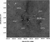Fig. 1 DSSR image of the brightest part of RCW 54. The image is  ~1$\stackrel{\mathrm{°}}{.}$5  ×  1$\stackrel{\mathrm{°}}{.}$5 in size, centered at (l, b) = (289$\stackrel{\mathrm{°}}{.}$5, 0$\stackrel{\mathrm{°}}{.}$25). Our region of interest is delimited by the white dashed square.

In their southern hemisphere catalog of bright-rimmed clouds (BRCs) associated with IRAS point sources, Sugitani & Ogura (1994) quote SFO 62 as related to NGC 3503. BRCs are defined as isolated molecular clouds located at the edges of evolved Hii regions, and are suspected of being potential sites of star formation through the radiation-driven implosion (RDI) process (Sugitani et al. 1991; Urquhart et al. 2009). Making use of the Australian Telescope Compact Array (ATCA), Thompson et al. (2004) carried out radio continuum observations toward all BRCs cataloged by Sugitani & Ogura (1994). These authors classified SFO 62 as a broken-rimmed cloud associated with an evolved stellar cluster that is about to disrupt its natal molecular cloud. Later on, Urquhart et al. (2009) claim that SFO62 was incorrectly classified as a BRC and that the RDI process is not working in this region.

Using the [Sii] λ6716/λ6731 line ratio of NGC 3503 , Copetti et al. (2000) detect a significant electron density dependence on position, which according to the authors, could be interpreted as a radial gradient. The authors claim that NGC 3503 may be a candidate for showing a “champagne flow”. In their Hα survey of the Milky Way toward l = 290°, Georgelin et al. (2000) report a radial velocity¹ of –21 km s^-1 toward NGC 3503 and propose that NGC 3503 is linked to a complex of Hii regions placed at a distance of about 2.7 kpc, with radial velocities of about  − 25 km s^-1 . Published distance determinations of NGC 3503 vary between a minimum of 2.6 kpc (Herbst 1975) and a maximum of 4.2 kpc (Moffat & Vogt 1975). In this paper we adopt a distance of 2.9  ±  0.4 kpc(Pinheiro et al. 2010).

NANTEN ¹³CO (J = 1 → 0) (HPBW = 2.7′) line observations were carried out by Yamaguchi et al. (1999) toward 23 Hii regions associated with 43 BRCs cataloged by Sugitani & Ogura (1994), with a grid spacing of  ~4′  ×  4′. The aim of that work was to investigate the dynamical effects of Hii regions statistically on their associated molecular clouds and star formation. A square region of  ~ 0$\stackrel{\mathrm{°}}{.}$4 in size towards NGC 3503 was observed, and a single and slightly extended 6′ diameter molecular cloud was found to have a peak radial velocity of –24.9 km s^-1 .After adopting a distance of 2.9 kpc, this molecular structure has a linear radious of 2 pc and a total mass of  ~500 M_⊙ . The authors rejected this cloud from the analysis sample, since it was detected at only one position. The ¹²CO, ¹³CO, and ¹⁸CO (J = 1 → 0) MOPRA position-switched observations were carried out by Urquhart et al. (2009). The ON position was centred on the position of the IRAS source associated with NGC 3503. The least abundant of the isotopes was not detected, while the emission lines of the other two isotopes show a double-peaked profile. From a Gaussian fitting, their peak radial velocities are  ~+20 km s^-1 and –25.6 km s^-1 .

Molecular line observations provide an invaluable support toward a better understanding of the interaction of Hii regions with their surroundings. Although providing important information about the molecular gas associated with NGC 3503 previous observations of Yamaguchi et al. (1999) and Urquhart et al. (2009), do not offer a complete picture of the molecular environment of the nebula. Bearing this in mind, the goals of this paper are twofold: a) to map the spatial distribution of the molecular gas associated with NGC 3503 and study its physical characteristics, and b) to achieve a better understanding of the interaction of NGC 3503 and Pis 17 with their molecular environment. These aims were addressed by analyzing new ¹²CO (J = 1 → 0) data gathered by using the NANTEN telescope to observe a square region  ~0$\stackrel{\mathrm{°}}{.}$6in size, centered on (l, b) = (289$\stackrel{\mathrm{°}}{.}$36, +0$\stackrel{\mathrm{°}}{.}$02). Molecular observations were combined with unpublished radio continuum data, and optical, mid-, and far-infraredarchival data.

The structure of the paper is the following. In Sect. 2, the CO and radio continuum observations are briefly described along with a short mention of the archival data used in this work. The main observational results of the molecular, ionized, and dust emission are detailed in Sect. 3, while both the comparison among these interstellar phases and the action of the stellar ionizing sources of NGC 3503 over its interstellar environs, as well as the star formation activity, are explained in Sect. 4. Finally, a possible scenario is put forward to explain the stellar and interstellar interactions. A summary is presented in Sect. 5.

2. Observations and data reductions

The databases used in this work are

• 1.

  Intermediate angular resolution, medium sensitivity, andhigh-velocity resolution ¹²CO (J = 1 → 0) data obtained with the 4-mNANTEN millimeter-wave telescope of Nagoya University. Atthe time the authors carried out the observations, April 2001, thistelescope was installed at Las Campanas Observatory, Chile. Thehalf-power beamwidth and the system temperature, includingthe atmospheric contribution toward the zenith, were2$\stackrel{\mathrm{\prime }}{.}$7 (~2.3 pc at 2.9 kpc) and  ~220 K (SSB) at 115 GHz, respectively. The data were gathered using the position-switching mode. Observations of points devoid of CO emission were interspersed among the program positions. The coordinates of these points were retrieved from a database that was kindly made available to us by the NANTEN staff. The spectrometer used was an acusto-optical with 2048 channels providing a velocity resolution of  ~0.055 km s^-1. For intensity calibrations, a room-temperature chopper wheel was employed (Penzias & Burrus 1973). An absolute intensity calibration (Ulich & Haas 1976; Kutner & Ulich 1981) was achieved by observing Orion KL (RA(1950.0) = 5^h32^m47$\stackrel{\mathrm{s}}{.}$0, Dec (1950.0) =  − 5°24′21′′), and ρ Oph East (RA(1950.0) = 16^h29^m20$\stackrel{\mathrm{s}}{.}$9, Dec (1950.0) =  − 24°22′13′′). The absolute radiation temperature, ${\mathit{T}}_{\mathrm{R}}^{\mathrm{\ast }}$, of Orion KL and ρ Oph East, as observed by the NANTEN radiotelescope, were assumed to be 65 K and 15 K, respectively (Moriguchi et al. 2001). The CO observations covered a region ( △ l  ×   △ b) of 35$\stackrel{\mathrm{\prime }}{.}$1  ×  35$\stackrel{\mathrm{\prime }}{.}$1 centered on (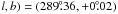$\mathit{l,b}\mathrm{)}\mathrm{=}\mathrm{(}\mathrm{289}\stackrel{\mathrm{°}}{.}\mathrm{36}\mathit{,}\mathrm{+}\mathrm{0}\stackrel{\mathrm{°}}{.}\mathrm{02}\mathrm{)}$, and the observed grid consists of points each located one beam apart. A total of 169 positions were observed. Typically, the integration time per point was 16s, resulting in an rms noise of  ~0.3 K. A second-order degree polynomial was substracted from the observations to account for instrumental baseline effects. The spectra were reduced using CLASS software (GILDAS working group).

• 2.

  Unpublished radio continuum data at 4800 and 8640 MHz which were kindly provided by J. S. Urquhartand M. A. Thompson. The images were obtained in March 2005 with the Australia Telescope Compact Array (ATCA) with synthesized beams of 23$\stackrel{\mathrm{″}}{.}$55  ×  18$\stackrel{\mathrm{″}}{.}$62and 14$\stackrel{\mathrm{″}}{.}$73  ×  11$\stackrel{\mathrm{″}}{.}$74at 4800 and 8640 MHz, respectively. The rms noises for these frequencies are 0.82 mJy beam^-1and 0.56 mJy beam^-1. Radio continuum archival images were also obtained from the Sydney University Molonglo Sky Survey (SUMSS)² (Bock et al. 1999) at 843 MHz, with angular resolution of 45′′ × 45′′ cosec(δ).

• 3.

  Infrared data retrieved from the Midcourse Space Experiment (MSX)³ (Price et al. 2001), high resolution IRAS images (HIRES)⁴ at 60 and 100 μm (Fowler & Aumann 1994), Spitzer images at 8.0 and 4.5 μm from the Galactic Legacy Infrared Mid-Plane Survey Extraordinaire (GLIMPSE)⁵ (Benjamin et al. 2003), and Multiband Imaging Photometer for Spitzer (MIPS) images at 24 and 70 μm from the MIPS Inner Galactic Plane Survey (MIPSGAL)⁶ (Carey et al. 2005).

• 4.

  Optical data retrieved from the 2nd Digitized Sky Survey (red plate)⁷ (McLean et al. 2000).

3. Results and analysis

3.1. Carbon monoxide

In order to illustrate in broad terms the molecular structures detected toward the region under study, a series of CO profiles are displayed in Fig. 2.

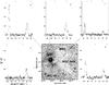Fig. 2 CO emission profiles toward five positions around NGC 3503. The CO profiles are averaged over a square area  ~ 3′ in size, centered on the black/white dots drawn in the DSSR image (center). The intensities are given as absolute radiation temperature ${\mathit{T}}_{\mathrm{R}}^{\mathrm{\ast }}$.

Profiles a) and c) show the CO emission along the line of sight to NGC 3503 and the bright edge of SFO 62 . In both spectra the bulk of the molecular emission is detected between –30and –20 km s^-1 and from +15 to +25 km s^-1 ,in good agreement with previous results by Urquhart et al. (2009).

The medium-brightness optical region northeast of NGC 3503  (from here onward MBO), however, also depicts a double peak structure (see profile b) and displays some small-scale structure in the feature peaking at  ~+20 km s^-1 ,while the most negative CO feature is detected at  ~ –18 km s^-1 .The molecular gas along regions of high optical absorption is shown in profiles d) and e). The former resembles the CO spectrum observed towards NGC 3503 , and is characteristic of the molecular emission in the region of high optical absorption seen northwest of NGC 3503 . The roundish patch of high absorption seen at (l, b) = (289$\stackrel{\mathrm{°}}{.}$55,+0$\stackrel{\mathrm{°}}{.}$07)only shows the CO peak at positive velocities.

The spatial distribution of the molecular gas observed in the three velocity intervals mentioned above is shown in the left hand panels of Fig. 3. In order of increasing radial velocity, the CO components are referred to as Component 1 (peaking at  ~–25 km s^-1 ), Component 2 (peaking at  ~–16 km s^-1 ), and Component 3 (peaking at  ~+20 km s^-1 ). To facilitate the comparison between the spatial distribution of molecular and ionized gas, the right hand panels of Fig. 3 show the same molecular contours as the left hand panels superimposed on the DSSR image in grayscale. The difference in spatial distribution among the three components is readily appreciated. The molecular gas in the velocity interval –29 to –20 km s^-1  (Component 1) shows two well developed concentrations, whose emission peaks are located at (l, b) = (289$\stackrel{\mathrm{°}}{.}$47,+0$\stackrel{\mathrm{°}}{.}$12)(clump A) and (l, b) = (289$\stackrel{\mathrm{°}}{.}$32′, +0$\stackrel{\mathrm{°}}{.}$03)(clump B). Component 1 has a very good morphological correspondence with the high optical obscuration region seen north and northwest of NGC 3503 .

Component 2 peaks at (l, b) = (289$\stackrel{\mathrm{°}}{.}$55, +0$\stackrel{\mathrm{°}}{.}$17)near both NGC 3503 and MBO and is projected onto a region without appreciable optical absorption. Finally, Component 3 (l, b) = (289$\stackrel{\mathrm{°}}{.}$45,  − 0$\stackrel{\mathrm{°}}{.}$18), does not show any clear morphological correspondence either with ionized regions or in areas displaying strong absorption.

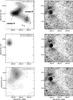Fig. 3 Upper panels (left): averaged ${\mathit{T}}_{\mathrm{R}}^{\mathrm{\ast }}$ in the velocity range  ~ –29 to –20 km s-1 (Component 1). Contour levels start at 0.42 K (23 rms) and the contour spacing is 0.6 K. The beam size of the CO observations is shown by a circle in the lower left corner. right: overlay of the ${\mathit{T}}_{\mathrm{R}}^{\mathrm{\ast }}$ values in the same velocity interval (contours), superimposed on the DSSR image (grayscale). Middle panels: averaged ${\mathit{T}}_{\mathrm{R}}^{\mathrm{\ast }}$ in the velocity range  ~–17.5 to –15.5 km s-1 (Component 2). Contour levels start at 0.7 K (23 rms) and the contour spacing is 1 K. Lower panels: averaged ${\mathit{T}}_{\mathrm{R}}^{\mathrm{\ast }}$ in the velocity range  ~+14 to +24 km s-1 (Component 3). Contour levels start at 0.35 K (23 rms) and the contour spacing is 0.45 K. In the left panels, the grayscale goes from 0.35 K to 3.9 K. The orientation of the equatorial system is indicated in the top left panel.

For the three molecular components, a mean radial velocity () weighted by line temperature was derived by means of 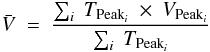$\begin{array}{ccc}\mathit{V̅}\mathrm{=}\frac{{\sum }_{\mathit{i}}{\mathit{T}}_{{\mathrm{Peak}}_{\mathit{i}}}\mathrm{\times }{\mathit{V}}_{{\mathrm{Peak}}_{\mathit{i}}}}{{\sum }_{\mathit{i}}{\mathit{T}}_{{\mathrm{Peak}}_{\mathit{i}}}}& & \end{array}$(1)where T_Peaki and V_Peaki are the peak ${\mathit{T}}_{\mathrm{R}}^{\mathrm{\ast }}$ temperature and the peak radial velocity of the i-spectrum observed within the 3 rms contour line defining the outer border. Mean radial velocities of –24.7 km s^-1 ,–16.6 km s^-1 ,and +19.5 km s^-1 were obtained for Component 1, 2, and 3, respectively.

Based on , we tried to estimate the kinematical distance of Component 1. The analytical fit to the rotation curve by Brand & Blitz (1993) along l = 289$\stackrel{\mathrm{°}}{.}$5 shows that radial velocities that are more negative than –15.5 km s^-1  are forbidden for this galactic longitude. However, the ionized gas along this galactic longitude exhibits velocity departures that are more negative than  − 7 km s^-1 relative to the circular rotation model, such as the cases of the Hii  regions Gum 37 (l, b) = (290$\stackrel{\mathrm{°}}{.}$65, +0$\stackrel{\mathrm{°}}{.}$26)(d = 2.7 kpc)and Gum 38a (l, b) = (291$\stackrel{\mathrm{°}}{.}$28, +0$\stackrel{\mathrm{°}}{.}$71)(d = 2.8  kpc), whose radial velocities are in the range  − 25 to  − 28 km s^-1 and  − 25 to  − 29 km s^-1 ,respectively (Georgelin et al. 2000). Bearing in mind that, close to the tangential point along l = 290$\stackrel{\mathrm{°}}{.}$5, the radial velocity gradient is very small and that the Hii  regions located at distances between 2.7 and 2.8 kpc exhibit forbidden radial velocities similar to those found for Component 1, we adopt a distance of 2.9 ± 0.4 kpc for the latter (Pinheiro et al. 2010), which is also the kinematical distance corresponding to the tangential point.

Component 1 shows an excellent morphological resemblance to a region of high optical absorption next to NGC 3503 (see Fig. 3), and its mean velocity is in good agreement with the velocity of the Hα line towards the nebula ( − 21 km s^-1 ; Georgelin et al. 2000). It is also worth noting that the velocity interval of Component 1 is in excellent agreement with the velocity of SFO 62 found by Sugitani & Ogura (1994) (–28  ≤   v_LSR   ≤  –20 km s^-1 , at ¹²CO), by Yamaguchi et al. (1999) (–24.9 km s^-1 at ¹³CO), and by Urquhart et al. (2009) ( − 25.6 at ¹²CO and  − 25.7 km s^-1 at ¹³CO). Based on the above, we conclude that Component 1 is associated with NGC 3503 and its environs. The bright rim of SFO 62  clearly follows the southernmost border of clump A, which very likely indicates that the molecular gas on the southern border of this clump is being ionized, giving rise to the bright optical rim.

On the other hand, considering that the mean radial velocity of Component 2 (–16.5 km s^-1 ) is close to the radial velocity of the tangential point at l = 289$\stackrel{\mathrm{°}}{.}$5 (–15.5 km s^-1 ), we suggest that Component 2 may be located in the neighborhood of the tangential point, close to Component 1. From the mean radial velocity of Component 3, a kinematic distance of  ~ 8 kpc is determined, indicating that Component 3 is unrelated to NGC 3503 . Very likely, Component 3 is associated with the complex of Hii regions at a velocity of  ~ +20 km s^-1 (Georgelin et al. 2000).

A direct comparison of Component 1 with the molecular cloud detected by Yamaguchi et al. (1999)(see Fig. 2u from that work) shows that the angular size of Component 1 is about a factor 3–4 greater than the latter. Clearly, only the densest part of the molecular cloud associated with NGC 3503 (clump A) was detected in the ¹³CO observations of Yamaguchi et al. (1999). From here onwards, the analysis of the molecular gas associated with NGC 3503 focuses on Component 1.

The kinematics of Component 1 was studied by using position-velocity maps across selected strips. The map obtained along b = +0$\stackrel{\mathrm{°}}{.}$12(corresponding to clump A) is shown in the upper panel of Fig. 4. A noticeable velocity gradient is observed at velocities from about  − 23 km s^-1 to about  − 28 km s^-1 .

Fig. 4 Upper panel: velocity-galactic longitude map obtained in a strip along b = +0$\stackrel{\mathrm{°}}{.}$11 (corresponding to clump A) showing ${\mathit{T}}_{\mathrm{R}}^{\mathrm{\ast }}$. Contour levels start at 0.7 K and the contour spacing is 0.7 K. The dotted lines indicate the location of NGC 3503 . Lower panel: mean velocity map of Component 1. Contours levels go from  − 26 to  − 24 km s-1 , with interval of 0.2 km s-1 . The dotted ellipse depicts approximately the region of clump A.

Additional support for the existence of this gradient can be obtained through a moment analysis. Due to the large angular dimensions of Component 1 and the spatial sampling of NANTEN observations, 28 independent CO profiles were observed toward the region enclosed by the 0.42 K-contour line in Fig. 3. Since these spectra have a high signal-to-noise ratio (S/N > 10), they are well-suited to studying possible variations in the CO profiles across Component 1 in some detail. With this aim, we used the AIPS package to calculate the first three moments (integrated area, temperature weighted mean radial velocity, and velocity dispersion) of the CO profiles. In the lower panel of Fig.  4, the temperature-weighted, mean radial velocity distribution of CO is shown. A clear velocity gradient is observed along Component 1, particulary in the region of clump A (depicted by the dotted ellipse), with mean radial velocities more negative toward the position of NGC 3503 . A velocity shift of about  ~ 1.4 km s^-1 is observed across the region of clump A, which at a distance of 2.9 kpc translates to a gradient ω ≈ 0.15 km s^-1  pc^-1. This panel also shows that the CO emission corresponding to clump B does not show any significant velocity gradient.

To offer a complete picture of the kinematical properties of clump A, we show in Fig. 6 the spatial distribution of the CO emission within the velocity range from –27.4 to –23.4 km s^-1 . Each image depicts mean ${\mathit{T}}_{\mathrm{R}}^{\mathrm{\ast }}$-values (in contours) over a velocity interval of 1 km s^-1 superimposed on the 8.13 μm MSX  emission (in grayscale). In the velocity range from –27.4 to –26.4 km s^-1 ,the molecular emission arising from clump A is slightly displaced from the brightest MSX emission located at (l, b)  ≈  (289$\stackrel{\mathrm{°}}{.}$5, +0$\stackrel{\mathrm{°}}{.}$11). As we move toward more positive velocities, the maximum of the CO emission gradually shifts westward.

Following Urquhart et al. (2009), we analyzed the excitation temperature (T_exc) obtained from the CO data to probe the surface conditions of Component 1. The excitation temperature of the ¹²CO line can be obtained considering that ¹²CO is optically thick (τ_ν ≪ 1). Then, the peak temperature of this line is given by ${\mathit{T}}_{\mathrm{peak}}{\mathrm{(}}^{\mathrm{12}}\mathrm{CO}\mathrm{)}\mathrm{=}{\mathit{J}}_{\mathit{\nu }}\mathrm{(}{\mathit{T}}_{\mathrm{exc}}\mathrm{)}\mathrm{-}{\mathit{J}}_{\mathit{\nu }}\mathrm{(}{\mathit{T}}_{\mathrm{bg}}\mathrm{)}$(2)(Dickman 1978) where J_ν is the Planck function at a frequency ν. Assuming Gaussian profiles for the ¹²CO line, combining the order-zero moment map (i.e., integrated area) with the order-two moment map (i.e., velocity dispersion) and using Eq. (2), we obtain the T_exc distribution map (Fig. 5). As expected, the T_exc distribution is quite similar to the CO emission distribution of Component 1, reaching a maximum of  ~17.7 K at (l, b)  ≈  (289$\stackrel{\mathrm{°}}{.}$45, +0$\stackrel{\mathrm{°}}{.}$11). It is worth noting that the obtained value of T_exc toward the center of clump A is lower than the obtained by Urquhart et al. (2009) toward (l, b)  ≈  (289$\stackrel{\mathrm{°}}{.}$5, +0$\stackrel{\mathrm{°}}{.}$11)(T_exc = 23.9 K). This difference may be explained in terms of a beam smearing of our NANTEN data, which implies that the values of T_exc shown in Fig. 5 must be considered as lower limits.

Fig. 5 Spatial distribution of Texc for Component 1. Contours leves are 5.7, 7.9, 10.2, 12.4, 14.5, and 16.6 K.

Fig. 6 Overlay of mean ${\mathit{T}}_{\mathrm{R}}^{\mathrm{\ast }}$-values (contours) in the velocity range from  − 27.4 to  − 23.4 km s-1 and the MSX band A emission (grayscale). Every image represents the CO emission distribution averaged in a velocity interval of 1 km s-1. The velocity interval is indicated in the bottom right corner of each image. The lowest temperature contour is 0.84 K (~12 rms). The contour spacing temperature is 1.4 K.

The mass of the molecular gas associated with NGC 3503 can be derived by using the empirical relationship between the molecular hydrogen column density, N(H₂), and the integrated molecular emission, ${\mathit{I}}_{{\mathrm{12}}^{}\mathrm{CO}}$ ( ≡ ${}^{\mathrm{\int }}{\mathit{T}}_{\mathrm{R}}^{\mathrm{\ast }}\mathrm{d}\mathit{v}$). The conversion between ${\mathit{I}}_{{\mathrm{12}}^{}\mathrm{CO}}$ and N(H₂) is given by the equation $\mathit{N}\mathrm{\left(}{\mathrm{H}}_{\mathrm{2}}\mathrm{\right)}\mathrm{=}\mathrm{(}\mathrm{1.9}\mathrm{\pm }\mathrm{0.3}\mathrm{)}\mathrm{\times }{\mathrm{10}}^{\mathrm{20}}{\mathit{I}}_{\mathrm{12}\mathrm{CO}} \mathrm{\left(}{\mathrm{cm}}^{-2}\mathrm{\right)}$(3)(Digel et al. 1996; Strong & Mattox 1996). The total molecular mass M_tot, was calculated through ${\mathit{M}}_{\mathrm{tot}}\mathrm{=}\mathrm{(}{\mathit{m}}_{\mathrm{sun}}{\mathrm{)}}^{-1}\mathit{\mu }{\mathit{m}}_{\mathrm{H}}\begin{array}{}\sum \end{array}\mathrm{\Omega }\mathit{N}\mathrm{(}{\mathrm{H}}_{\mathrm{2}}\mathrm{)}{\mathit{d}}^{\mathrm{2}} \mathrm{(}{\mathit{M}}_{\mathrm{\odot }}\mathrm{)}$(4)where m_sun is the solar mass (~2 × 10³³ g), μ the mean molecular weight, assumed to be equal to 2.8 after allowance of a relative helium abundance of 25% by mass (Yamaguchi et al. 1999; Yamamoto et al. 2006), m_H is the hydrogen atom mass (~1.67 × 10^-24 g), Ω the solid angle subtended by the CO feature in ster, d the distance expressed in cm, and M_tot is given in solar masses. For Component 1, we obtain a mean column density of N(H₂) = (1.9  ±  0.3)  ×  10²¹ cm^-2 and a total molecular mass of M_tot = (7.6  ±  2.1)  ×  10³M_⊙ . The uncertainty in M_tot (~28 %) stems from the distance uncertainty and from the error quoted for the coefficient in Eq. (3). Areas having ${\mathit{T}}_{\mathrm{R}}^{\mathrm{\ast }}\mathrm{\ge }\mathrm{0.42}$ K were taken into account. The difference with the value derived by Yamaguchi et al. (1999) (500 M_⊙ ) is due to both the subsampled observations of these authors and the fact that ¹³CO line is a better tracer of high-density regions.

The mean volume density (n_H2) of Component 1 can be derived from the ratio of its molecular mass and its volume considering that the volume of Component 1 is the result of the addition of an ellipsoid with major and minor axes of 7$\stackrel{\mathrm{\prime }}{.}$5 and 4$\stackrel{\mathrm{\prime }}{.}$5, respectively, centered at (l, b)  ≈  (289$\stackrel{\mathrm{°}}{.}$42, +0$\stackrel{\mathrm{°}}{.}$15)(which includes clump A), and a sphere of 4$\stackrel{\mathrm{\prime }}{.}$5 in radius, centered at (l, b)  ≈  (289$\stackrel{\mathrm{°}}{.}$33, +0$\stackrel{\mathrm{°}}{.}$04)(which includes clump B). We derived n_H2  ≈  400 cm^-3. Taking the mass and volume uncertainties into account, we derive a conservative density error of about 60% (~240 cm^-3).

3.2. Radio continuum emission

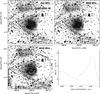Fig. 7 Upper left panel: radio continuum image at 843 MHz (contours) superimposed on the DSSR image (grayscale). Contours levels go from 4 mJy beam-1 (~3 rms)to 12 mJy beam-1 in steps of 4 mJy beam-1, and from 20 mJy beam-1 in steps of 10 mJy beam-1. Upper right panel: radio continuum image at 4800 MHz (contours) superimposed to the DSSR image (grayscale). Contours levels go from 2.4 mJy beam-1 (~3 rms)to 10.4 mJy beam-1 in steps of 2 mJy beam-1, and from 10.4 mJy beam-1 in steps of 4 mJy beam-1. The symmetry axis of the nebula is depicted by the dotted line. Lower left panel: radio continuum image at 8640 MHz (contours) superimposed to the DSSR image (grayscale). Contours levels go from 15 mJy beam-1 (~3 rms)in steps of 1 mJy beam-1. Lower right panel: emission measure profile obtained from the 4800 MHz radio continuum image along the symmetry axis of NGC 3503 .

Figure 7 shows the radio continuum images at 843, 4800, and 8640 MHz (in contours) superimposed on the DSSR image in a region of  ~9′  ×  9′ centred on NGC 3503 . The continuum images show an extended source coincident with NGC 3503 . The maxima at the three frequencies coincide with the brightest optical emission region. The source, which has a good morphological correspondence with the optical emission, exhibits a cometary shape with its symmetry axis in the image at 4800 MHz (Fig. 7, top right panel). The fainter emission area detected at 843 and 4800 MHz to the northeast of NGC 3503 coincides with MBO and appears to be linked to the emission of the nebula at (l, b)  ≈  (289$\stackrel{\mathrm{°}}{.}$53, +0$\stackrel{\mathrm{°}}{.}$13). The emission region detected at (l, b)  ≈  (289$\stackrel{\mathrm{°}}{.}$48, +0$\stackrel{\mathrm{°}}{.}$08)at 843 MHz depicts some morphological correspondence with the bright rim of SFO 62. The point-like source placed at (l, b)  ≈  (289$\stackrel{\mathrm{°}}{.}$49,+0$\stackrel{\mathrm{°}}{.}$15)without optical emission counterpart is labeled G289.49+0.15 in Fig. 7. From its flux densities F₈₄₃ = 100 mJy, F₄₈₀₀ = 17.1 mJy, and F₈₆₄₀ = 11.5 mJy, we derived a spectral index α = –0.92  ±  0.03(S_ν  ∝  ν^α), which suggests that G289.49+0.15 is a nonthermal extragalactic source. We substracted the emission of this source in order to calculate radio continuum flux densities of NGC 3503 . The results are given in Table 1. The spectral index based on these estimates is α =  − 0.12  ±  0.03, typical of the thermal free-free radio continuum emission of an Hii region.

We estimated the emission measure EM${\mathrm{(}}^{}\mathrm{=}{}^{\mathrm{\int }}\mathit{n}_{\mathrm{e}}^{\mathrm{2}}\mathrm{d}{\mathit{l}}^{\mathrm{)}}$ along the symmetry axis of the nebula using the image at 4800 MHz. The brightness temperature (T_b) is related to the optical depth (τ) by $\begin{array}{ccc}{\mathit{T}}_{\mathrm{b}}\mathrm{\left(}\mathit{\nu }\mathrm{\right)}\mathrm{=}{\mathit{T}}_{\mathrm{e}}\mathrm{\times }\mathrm{(}\mathrm{1}\mathrm{-}{\mathrm{e}}^{\mathrm{-}\mathit{\tau }}\mathrm{)}& & \end{array}$(5)where T_e = 8100 ± 700 K (Quireza et al. 2006) is the electron temperature, and the optical depth τ is given by $\begin{array}{ccc}\mathit{\tau }\mathrm{=}\mathrm{8.235}\mathrm{\times }{\mathrm{10}}^{-2}{\mathit{T}}_{\mathrm{e}}^{-1.35}{\mathit{\nu }}^{-2.1}\mathit{EM}\mathit{.}& & \end{array}$(6)In this last expression, ν is given in GHz and EM in pc cm^-6. The EM profile is shown in the lower right hand panel of Fig. 7. As expected, two maxima are observed, one in the brightest section of NGC 3503 and the other coincident with MBO, indicating that the electron density is higher toward these regions than in the sorroundings. The EM profile of NGC 3503 is consistent with the cometary shape morphology of the nebula seen in the radio continuum and optical images. The EM profile shows a sharp border toward the west of the nebula, while toward the east it decreases smoothly, indicating the existence of an electron density gradient. The observed EM profile agrees with the results of Copetti et al. (2000), who report an electron density gradient in the east-west direction. Using the peak values EM = 18 000 pc cm^-6(obtained at (l, b)  ≈  (289$\stackrel{\mathrm{°}}{.}$50, +0$\stackrel{\mathrm{°}}{.}$11)for NGC 3503 ) and EM = 7000 cm^-6(obtained at (l, b)  ≈  (289$\stackrel{\mathrm{°}}{.}$53, +0$\stackrel{\mathrm{°}}{.}$18)for MBO), and considering a pure hydrogen plasma with a depth along the line of sight equal to the size in the plane of the sky, an electron density estimates of n_e = 75  ±  14 cm^-3is obtained for NGC 3503 and n_e = 45  ±  9 cm^-3for MBO.

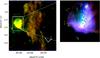Fig. 8 Left panel: composite image of NGC 3503 and its environs. Red and green show emission at 8.13 μm (MSX) and 24 μm (MIPSGAL). The color scale goes from 1 × 10-5 to 4 × 10-5 W m-2 sr-1and from 27 to 100 MJy ster-1, respectively. The white rectangle encloses the IR counterpart of NGC 3503 (IRK). Right panel: composite image of NGC 3503 . Red, green, and blue show emission at 8 μm (IRAC-GLIMPSE), 24, and 70 μm (MIPSGAL), respectively. Colors scales range from 40 to 500 MJy ster-1(24 μm), from 300 to 2000 MJy ster-1(70 μm), and from 30 to 400 MJy ster-1(8 μm). The location of the members of Pis 17 is indicated with black crosses. MSX and 2MASS candidate YSOs are indicated with red and green crosses (see text).

As a different approach to NGC 3503 , the rms electron density and ionized mass can be obtained using the spherical model of Mezger & Henderson (1967) and the flux density at 4800 MHz. Assuming a constant electron density, and a radius R_HII = 1.25 pc, we obtain n_e = 54  ±  13 cm^-3and M_HII = 11  ±  3 M_⊙ . Thus, the electron density of NGC 3503 is about a factor of 5 lower than the density of Component 1, which clearly indicates that the nebula has expanded. An estimate of the filling factor (f = $\sqrt{{\mathit{n}}_{\mathrm{e}}\mathit{/}{\mathit{n}}_{\mathrm{e}}^{\mathrm{\prime }}}$)can be obtained by taking the maximum electron density derived from optical lines into account (${\mathit{n}}_{\mathrm{e}}^{\mathrm{\prime }}$ = 154$\begin{array}{}\mathrm{+}\mathrm{52}\\ -45\end{array}$ cm^-3; Copetti et al. 2000). We obtain f = 0.5 − 0.8. Then, the ionized mass for f = 0.5 − 0.8 is in the range 8 − 10 M_⊙ .

Regarding MBO, rms electron densities and masses estimated from the image at 843 MHz are n_e  ≃  33 cm^-3and M_HII  ≃  6 M_⊙ .

3.3. Infrared emission

The emission distribution at 8.13 μm (MSX-A band) superposed on the image at 24 μm (MIPSGAL) is shown in the left hand panel of Fig. 8. The MSX Band A includes the strong emission features at 7.7 and 8.6 μm attributed to PAH molecules, which are considered tracers of UV-irradiated PDR (Hollenbach & Tielens 1997). This image displays a small and strong feature, from here on dubbed the IR Knot, or IRK for short (indicated with a white rectangle), which is coincident with the location of NGC 3503 , and a weaker and more extended emission region detected in the northwestern area of the image. The last feature is referred to as the extended IR emission (EIE). The IR emission at 8.3 and 24 μm appears mixed along the whole feature. A region of low IR emission is seen between the IRK and the EIE. The bright rim of SFO 62 is detected in the IR as the bright filament observed from (l,b)  ≃  (289$\stackrel{\mathrm{°}}{.}$42, +0$\stackrel{\mathrm{°}}{.}$03)to (l,b)  ≃  (289$\stackrel{\mathrm{°}}{.}$50, +0$\stackrel{\mathrm{°}}{.}$08), which appears to be the southernmost boundary of EIE. The presence of PAH emission coincident with this bright rim suggests there is a PDR at the southern edge of Component 1.

The right hand panel of Fig. 8 shows a detailed image of the IRK at 8.0 μm (Spitzer-IRAC band 4), 24 μm (MIPSGAL), and 70 μm (MIPSGAL, in blue). The emissions at 8 and 70 μm show a bright half shell-like feature, which encloses the position of the stars of Pis 17. Arc-shaped faint filaments are also detected in the 8 μm emission in the northeastern section of IRK. The morphology of the IR emission is compatible with the cometary-shape of the Hii region and very likely indicates a PDR between NGC 3503 and clump A. The MIPSGAL emission at 24 μm, which is projected onto the center of the structure, indicates the existence of warm dust inside the Hii region (such as the cases of N10 and N21, Watson et al. 2008).

Fig. 9 Upper panel: Td distribution estimated from HIRES IRAS images at 60 and 100 μm. Contour levels go from 25 to 31 K in steps of 1 K, and from 33 K in steps of 2 K. Lower panel: overlay of the Td distribution (contours) and the DSSR image.

IRAS 60 and 100 μm data show dust with color temperatures between about 20 to 100 K, which corresponds to the “cool dust component” (see Sreenilayam & Fich 2011, and references therein). A dust temperature (T_d) map was produced using the equation ${\mathit{T}}_{\mathrm{d}}\mathrm{=}\mathrm{95.94}\mathit{/}\ln \mathrm{\left(}{\mathit{B}}_{\mathit{n}}\mathrm{\right)} \mathrm{\left(}\mathrm{K}\mathrm{\right)}$(7)(Draine 1990; Whittet 1992; Cichowolski et al. 2001), where B_n = 1.667⁽³⁺ⁿ⁾${}^{\mathrm{(}}\mathit{F}_{\mathrm{100}}\mathit{/}{\mathit{F}}_{\mathrm{60}}{\mathrm{)}}^{}$ is the modified Planck function, with F₁₀₀ and F₆₀ the 100 μm and 60 μm fluxes. The parameter n = 1.5 is related to the absorption efficiency of the dust (k_ν   ∝   νⁿ, normalized to 40 cm² g^-1 at 100 μm). The obtained dust temperature map is shown in the upper panel of Fig. 9. The dust temperature goes from 25 K to 46 K. Figure 9 (lower panel) also shows that the region with the highest dust temperatures (~46 K) coincides with the brightest section of NGC 3503 . This temperature is in good agreement with those obtained in RCW 121 and RCW 122 (Arnal et al. 2008) and in NGC 6357 (Cappa et al. 2011), although they are slightly higher than typical values for Hii regions (~30 K)(see Cappa et al. 2008; Cichowolski et al. 2009; Vasquez et al. 2010). The stellar UV radiation field of the stars in NGC 3503 is responsible for heating the dust immersed in the Hii region. A noticeable feature is a fringe of cold (~25 K) dust surrounding the position of NGC 3503 , which coincides with the region showing low emission at 8.3 μm placed between IRK and EIE described above. An extended region of warmer (~36 K) dust is detected to the northeast of NGC 3503 , coincident with the position of MBO, indicating that this optical feature has a radiatively heated dust component. In Table 2 we summarized the IR and dust parameters for IRK and EIE. The averaged dust temperatures () are calculated using Eq. (7) and flux densities at 60 and 100 μm obtained integrating several polygons around the sources. Dust masses are derived from ${\mathit{M}}_{\mathrm{d}}\mathrm{=}{\mathit{m}}_{\mathit{n}}{\mathit{F}}_{\mathrm{60}}{\mathit{d}}^{\mathrm{2}}\mathrm{(}{\mathit{B}}_{\mathit{n}}^{\mathrm{2.5}}\mathrm{-}\mathrm{1}\mathrm{)} \mathrm{\left(}{\mathit{M}}_{\mathrm{\odot }}\mathrm{\right)}$(8)where d the distance in kpc, F₆₀ is given Jy, and m_1.5 = 0.3  ×  10^-6. Based on the molecular gas mass derived for Component 1, the ionized gas of NGC 3503 and MBO, and the dust masses obtained for the IRK and the EIE (~10 M_⊙ ), we derive a mean weighted gas-to-dust ratio of about  ~ 800  ±  300. This ratio is a factor of about  ~5 higher than the average values assumed for the Galaxy (140 ± 50; Tokunaga 2000), however, dust with temperatures T_d   ≲   20 K (“cold dust component”), which is detected at wavelengths not surveyed by IRAS (λ  >  100 μm), dominates the dust mass by a factor greater than  ~ 70 with respect to the cool dust component (Sreenilayam & Fich 2011). This notoriously decreases the gas-to-dust ratio. The dust temperature estimated for EIE may suggest the existence of ionizing sources inside Component 1. However, a search for OB stars embedded in Component 1 performed using the available VizieR catalogs failed to detect such sources.

To investigate the presence of protostellar candidates possibly related to NGC 3503, we used data from the MSX, 2 MASS, and IRAS point source catalogs. We searched for point sources in a region of about 10′ in size centered on the position of the Hii  region. After taking sources with flux quality q > 2 into account, a total of 69 MSX point sources were found projected onto the area. Based on F₂₁/F₈ and F₁₄/F₁₂ ratios, where F₈, F₁₂, F₁₄, and F₂₁ are the fluxes at 8.3, 12, 14, and 21 μm, respectively, and after applying the criteria summarized by Lumsden et al. (2002), we were left with three sources with F₂₁/F₈ > 2 and F₁₄/F₁₂ < 1, which are classified as compact Hii regions (CHii ). This is indicative of stellar formation. The location of these sources is indicated with red crosses in Fig. 8.

Using the 2 MASS catalog (Cutri et al. 2003), which provides detections in J, H and K_s bands, we searched for point sources with infrared excess. Taking into account sources with signal-to-noise ratio (S/N) > 10 (corresponding to quality “AAA”), we found 5528 sources projected onto a circular region of 5′ in radius. Following Comerón et al. (2005), we determined the parameter q = (J − H) − 1.83 × (H − K_s). Sources with q <  −0.15 are classified as objects with infrared excess , i.e. candidate young stellar objects (YSOs). By applying the above criteria, we found only nine sources projected onto NGC 3503 . The location of these sources is also indicated in Fig. 8 with green crosses. The location of the 2 MASS source 11011390-5949099 (source #12) is almost coincident with the MSX source G289.4859+00.1420 (source #1). These sources are projected onto an intense mid-IR clump, located on the northeastern border of the bright half shell-like feature, at (l,   b) = (289$\stackrel{\mathrm{°}}{.}$48, +0$\stackrel{\mathrm{°}}{.}$14 )(see Fig. 8, right panel), and onto a small enhancement in the radio continuum emission detected at 4800 MHz (see Fig. 10 below). These characteristics make this object an excellent candidate for investigating star formation with high angular resolution observations. The names of the candidate YSOs, their position, fluxes, and magnitudes at different IR wavelengths are listed in Table 3.

4. Discussion

4.1. The ionized gas

The number of ionizing Lyman continuum photons (N_Lyc) needed to sustain the ionization in NGC 3503 can be calculated using the equation given by Simpson & Rubin (1990)$\begin{array}{ccc}{\mathit{N}}_{\mathrm{Lyc}}\mathrm{=}\mathrm{4.45}\mathrm{\times }{\mathrm{10}}^{\mathrm{48}}{\mathit{T}}_{\mathrm{e}}^{-0.45}{\mathit{S}}_{\mathrm{(}\mathrm{4800}\mathrm{MHz}\mathrm{)}}{\mathit{d}}^{\mathrm{2}}& & \end{array}$(9)where d is the distance in kpc, and S_{(4800  MHz)} the flux density at 4800 MHz in Jy. We obtain N_Lyc = (1.8  ±  0.4)  ×  10⁴⁷ s^-1. This number is a lower limit to the total number of Lyman continuum photons required to maintain the gas ionized, since about 25–50% of the UV photons are absorbed by interstellar dust in the Hii region (Inoue 2001). Consequently, we need N_Lyc  ≈  3.6  ×  10 ⁴⁷ s^-1. The number of Lyman continuum photons emitted by a B0 V star is ${\mathit{N}}_{\mathrm{Lyc}}^{\mathrm{\ast }}$ = 1.07  ×  10⁴⁸ s^-1 (Sternberg et al. 2003), which is capable of ionizing NGC 3503 , in agreement with previous results by Thompson et al. (2004) and Pinheiro et al. (2010). The last authors asserted one B0 V star and three B2 V stars belonging to the open cluster Pis17 inside the nebula,as ionizing sources. Since the ionizing photons emitted by a B2 V star are far fewer than those of a B0 V star, their contribution to the energetics of the nebula can be neglected.

In Sect. 3.2 we pointed out the discrepancy between the electron and molecular densities. The density of Component 1 is about a factor of 5 higher than the electron density of NGC 3503 , which clearly indicates that NGC 3503 has been expanding as a result of unbalanced pressure between ionized and molecular gas. To estimate the dynamical age (t_dyn) of the Hii region, we used the model of Dyson & Williams (1997). The radius of an Hii region (R_HII) in a uniform medium is given by 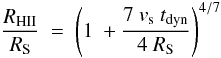$\frac{{\mathit{R}}_{\mathrm{HII}}}{{\mathit{R}}_{\mathrm{S}}}\mathrm{=}{\left(\mathrm{1}\mathrm{+}\frac{\mathrm{7}{\mathit{v}}_{\mathrm{s}}{\mathit{t}}_{\mathrm{dyn}}}{\mathrm{4}{\mathit{R}}_{\mathrm{S}}}\right)}^{\mathrm{4}\mathit{/}\mathrm{7}}$(10)where R_S is the radius of the Strömgren sphere (Strömgren 1939) before expanding, given by 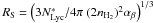${\mathit{R}}_{\mathrm{S}}\mathrm{=}{\left(\mathrm{3}{\mathit{N}}_{\mathrm{Lyc}}^{\mathrm{\ast }}\mathit{/}\mathrm{4}\mathit{\pi }\mathrm{(}\mathrm{2}{\mathit{n}}_{{\mathrm{H}}_{\mathrm{2}}}{\mathrm{)}}^{\mathrm{2}}{\mathit{\alpha }}_{\mathit{\beta }}\right)}^{\mathrm{1}\mathit{/}\mathrm{3}}$ , and v_s is the sound speed in the ionized gas (~10 km s^-1 ). For R_HII  ≃  1.25 pc(1$\stackrel{\mathrm{\prime }}{.}$5 at a distance of 2.9 kpc), an ambient density n_H2 = 400  ±  240 cm^-3(see Sect. 3.1.3), and ${\mathit{N}}_{\mathrm{Lyc}}^{\mathrm{\ast }}\mathrm{=}\mathrm{1.07}\mathrm{\times }{\mathrm{10}}^{\mathrm{48}}$ s^-1, we infer t_dyn  ≈  2  ×  10⁵yr. The expansion velocity of the Hii region can be estimated by means of Ṙ_HII = v_s${{}^{\mathrm{\right(}}\frac{{\mathit{R}}_{\mathrm{HII}}}{{\mathit{R}}_{\mathrm{s}}}^{\mathrm{\left)}}}^{\mathrm{-}\mathrm{3}\mathit{/}\mathrm{4}}$, yielding an expansion velocity of about  ~ 5 km s^-1. The obtained dynamical age and expansion velocity agree with those obtained in typical Hii regions (Gum 31, Cappa et al. 2008; Sh2-173, Cichowolski et al. 2009).

The total number of ionizing Lyman continuum photons needed to sustain the ionization in MBO is N_Lyc  ≈  2.5  ×  10⁴⁷ seg^-1. To search for stars that can provide the necessary UV photons, we used the available VizieR catalogs. CP-59 2951 is a B1 V star placed at (l, b) = (289$\stackrel{\mathrm{°}}{.}$511, +0$\stackrel{\mathrm{°}}{.}$195)(Buscombe & Foster 1999). Using the cataloged spectral type, the visual magnitude, and the calibration of Schmidt-Kaler (1982), we estimated a distance d = 2.7  ±  0.8 kpc. The continuum ionizing photons emitted by the star are ${\mathit{N}}_{\mathrm{Lyc}}^{\mathrm{\ast }}$ = 3.2  ×  10⁴⁶ s^-1(Smith et al. 2002). Although the distance of this star agrees (within errors) with the distance of NGC 3503 , the value of ${\mathit{N}}_{\mathrm{Lyc}}^{\mathrm{\ast }}$ is almost one order of magnitude lower than required to ionize MBO. The presence of Pis17 at a projected distance of 3.4 pc (~4′ at a distance of 2.9 kpc) indicates that the contribution of the star cluster to the ionization of MBO cannot be ruled out.

4.2. Star formation process

In Sect. 3.3 we reported twelve candidate YSOs that are projected onto the region of NGC 3503 . This suggests that they may have been triggered by the expansion of the Hii region through the “collect and collapse” model, which indicates that expanding nebulae compress gas between the ionization and the shock fronts, leading to the formation of molecular cores where new stars can be embedded. Using the analytical model of Whitworth et al. (1994) for the case of expanding Hii regions, we derived the time when the fragmentation may have occurred (t_frag), and the size of the Hii region at t_frag (R_frag), which are given by $\begin{array}{ccc}{\mathit{t}}_{\mathrm{frag}}\mathrm{\left[}{\mathrm{10}}^{\mathrm{6}} \mathrm{yr}\mathrm{\right]}\mathrm{=}\mathrm{1.56}{\mathit{a}}_{\mathrm{2}}^{\mathrm{4}\mathit{/}\mathrm{11}}{\mathit{n}}_{\mathrm{3}}^{\mathrm{-}\mathrm{6}\mathit{/}\mathrm{11}}{\mathit{N}}_{\mathrm{49}}^{\mathrm{-}\mathrm{1}\mathit{/}\mathrm{11}}& & \end{array}$(11)and $\begin{array}{ccc}{\mathit{R}}_{\mathrm{frag}}\mathrm{\left[}\mathrm{pc}\mathrm{\right]}\mathrm{=}\mathrm{5.8}{\mathit{a}}_{\mathrm{2}}^{\mathrm{4}\mathit{/}\mathrm{11}}{\mathit{n}}_{\mathrm{3}}^{\mathrm{-}\mathrm{6}\mathit{/}\mathrm{11}}{\mathit{N}}_{\mathrm{49}}^{\mathrm{1}\mathit{/}\mathrm{11}}\mathit{,}& & \end{array}$(12)where a₂ is the sound velocity in units of 0.2 km s^-1 , n₃ ≡ n_H2/1000, and ${\mathit{N}}_{\mathrm{49}}\mathrm{\equiv }{\mathit{N}}_{\mathrm{Lyc}}^{\mathrm{\ast }}\mathit{/}{\mathrm{10}}^{\mathrm{49}}$. Adopting 0.3 km s^-1 for this region for the sound velocity, which corresponds to temperatures of 10–15 K in the surrounding molecular clouds (see Sect. 3.1.2), we obtained t_frag ~ 3.5 × 10⁶ yr, and R_frag ~ 7.5 pc. Considering that the values of t_frag and R_frag are higher than t_dyn and R_HII (see Sect. 4.1), we can conclude that the fragmentation at the edge of NGC 3503 is doubtful.

4.3. Kinematics of clump A

In Sect. 3.2 we reported a velocity gradient across clump A. Velocity gradients in molecular cores/clumps were usually interpreted as gravitationally bound rotation motions (particulary in dense and small molecular cores). Several theoretical models predict cloud flattening perpendicular to the rotation axis in response to centrifugal stress, which at first glance seems to be suitable for clump A. To investigate the dynamical stability of clump A, we use the parameter β defined by Goodman et al. (1993) to quantify the dynamical role of rotation by comparing the rotational kinetic energy to the gravitational energy. Thus, β can be written as 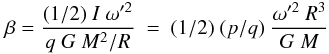$\mathit{\beta }\mathrm{=}\frac{\mathrm{(}\mathrm{1}\mathit{/}\mathrm{2}\mathrm{)}\mathit{I}{\mathit{\omega }}^{\mathrm{\prime }\mathrm{2}}}{\mathit{q}\mathit{G}{\mathit{M}}^{\mathrm{2}}\mathit{/}\mathit{R}}\mathrm{=}\mathrm{(}\mathrm{1}\mathit{/}\mathrm{2}\mathrm{)}\mathrm{(}\mathit{p}\mathit{/}\mathit{q}\mathrm{)}\frac{{\mathit{\omega }}^{\mathrm{\prime }\mathrm{2}}{\mathit{R}}^{\mathrm{3}}}{\mathit{G}\mathit{M}}$(13)where I is the moment of inertia (I = pMR²), qGM²/R is the gravitational potential energy, and ω′ = ω/sin(i), where i is the inclination of the cloud along the line of sight. Considering p/q=0.22(see Goodman et al. 1993), sin(i) = 1, ω = 0.15 km s^-1 pc^-1(see Sect. 3.1.2), R ~ 4.5 pc, and a lower limit mass to clump A (M ~ 3 × 10³M_⊙ ), we obtain β   ≈  0.02. This extremely low value of β indicates that the effect of rotation, if it exists, is not significant for mantaining the dynamical stability of clump A. This might weaken the rotating cloud interpretation. Furthermore, Figs. 4 and 6 show that only molecular gas at more negative velocities (~−27 km s^-1 / − 26 km s^-1 ) coincides with NGC 3503 , which suggests that the velocity gradient might be a direct consequence of an interaction between clump A and NGC 3503 .

Therefore, although rotation cannot be entirely ruled out with the present data, we consider different origins for the velocity gradient observed across clump A; namely, 1) the expansion of the nebula at  ~5 km s^-1 (see Sect. 4.1) has been accumulating molecular gas of clump A behind the shock front and expanding it at approximately the same velocity as the ionized gas, as expected according to the models of Hosokawa & Inutsuka (2006), 2) the velocity gradient of clump A is the consequence of a collision between Component 1 and another molecular cloud, which in turn might have induced the formation of Pis 17 and the candidate YSOs reported in Sect. 3.3. Although they are rare, cloud-cloud collisions can lead to gravitational instabilities in the dense, shocked gas, resulting in triggered star formation (see Elmegreen 1998, and references therein), 3) clump A is actually composed of different subclumps at different velocities, which are not resolved by the NANTEN observations. In this case, NGC 3503 might be related to a subclump at more negative velocities.

Further high-resolution studies with instruments like APEX may help to clarify this question.

4.4. The PDR at the interface between NGC 3503 and clump A

As mentioned in Sect. 3.1.2, clump A exhibits an excitation temperature T_exc ≥ 17.7 K, which is also the highest excitation temperature along Component 1. This temperature is higher than expected inside molecular cores if only cosmic ray ionization is considered as the main heating source (T ~ 8–10 K, van der Tak & van Dishoeck 2000), which implies that additional heating processes are present close to clump A. Very likely, clump A is being externally heated through the photoionisation of its surface layers (Urquhart et al. 2009) as a consequence of its proximity to NGC 3503 . This scenario is in line with the presence of the PDR at the interface between NGC 3503 and clump A (see Sect. 3.3). In this context, it would be instructive to make a simple comparison of the PDR dust surface temperature, with the dust temperature obtained before towards the edge of NGC 3503 (see Fig. 9).

The structure of a PDR is governed by the intensity of the UV radiation field impinging upon the cloud surface (G₀) in units of the Habing (1968) FUV flux (1.6 × 10^-3 erg cm^-2 s^-1), with 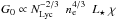${\mathit{G}}_{\mathrm{0}}\mathrm{\propto }{\mathit{N}}_{\mathrm{Lyc}}^{\mathrm{-}\mathrm{2}\mathit{/}\mathrm{3}}{\mathit{n}}_{\mathrm{e}}^{\mathrm{4}\mathit{/}\mathrm{3}}{\mathit{L}}_{\mathit{\star }}\mathit{\chi }$ (Tielens 2005), where χ is the fraction luminosity over 6 eV, and L _⋆  is the luminosity of the star. By adopting N_Ly = 1.07 × 10⁴⁸ s^-1 and L = 7.6 × 10⁴ L_⊙ (Sternberg et al. 2003), χ = 1, and considering n_e ≃ 75–154 cm^-3 (see Sect. 3.2), a range of G₀ ≃  (0.5–1.5)  ×  10³ is obtained. The distribution of dust temperature in the PDR (${\mathit{T}}_{\mathrm{d}}^{\mathrm{pdr}}$) is governed by the absorption of the stellar photons that are reemited by dust grains as IR photons. Following Tielens (2005), we can relate ${\mathit{T}}_{\mathrm{d}}^{\mathrm{pdr}}$ to the visual absorption along the PDR (A_v) as $\mathrm{(}{\mathit{T}}_{\mathrm{d}}^{\mathrm{pdr}}{\mathrm{)}}^{\mathrm{5}}\mathrm{\simeq }{\mathit{\nu }}_{\mathrm{0}}{\mathit{G}}_{\mathrm{0}}{\mathrm{e}}^{\mathrm{(}\mathrm{-}\mathrm{1.8}{\mathit{A}}_{\mathrm{v}}\mathrm{)}}\mathrm{+}\ln \mathrm{(}\mathrm{3.5}\mathrm{\times }{\mathrm{10}}^{-2}{\mathit{\tau }}_{\mathrm{100}}{\mathit{T}}_{\mathrm{0}}\mathrm{)}{\mathit{\tau }}_{\mathrm{100}}{{\mathit{T}}_{\mathrm{0}}}^{\mathrm{6}}$(14)where ν₀ is the frequency at 0.1  μm, τ₁₀₀ = 10^-3 the effective optical depth at 100 μm, and T₀ is the temperature of the slab estimated as T₀ = 12.2 G₀^1/5. Considering both, the position of NGC 3503 at the edge of clump A and the low value of visual absorption derived for the members of Pis 17 ( mag, Pinheiro et al. 2010) are probably due to the interstellar absorption in the line of sight of the Hii region, we can assume A_v ~  0 for the surface of the PDR. Taking the range of G₀ and Eq. (14) into account, we obtain ${\mathit{T}}_{\mathrm{d}}^{\mathrm{pdr}}\mathrm{\simeq }\mathrm{40}$–55 K, in accordance with the observed dust color temperature estimated for NGC 3503 (~46 K). This gives additional support to the existence of a PDR between NGC 3503 and clump A.

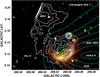Fig. 10 Composite image of NGC 3503 and its environs. Red and green show emission at 8 and 4.5 μm (IRAC-GLIMPSE), respectively. White and light blue contours show the radiocontinuum 4800 MHz and CO line emission.

4.5. Possible scenario

Figure 10 displays a composite image of NGC3503 and its environs with the radio continuum emission at 4800 MHz corresponding to NGC3503 and MBO and the CO emission. The color scale shows the emission at 8 μm and 4.5 μm.

As described in Sects. 3.3 and 4.3, emission attributed to PAHs encircles the southern and western borders of the Hii region, indicating the location of the PDR. The position of NGC 3503 near the border of clump A and the existence of an electron density gradient along the symmetry axis of the Hii region (with the higher electron densities close to the strongest CO emission) suggest that the ionised gas is being streamed away from the densest part of the molecular cloud. This is indicative that NGC 3503 is a blister-type Hii region (Israel 1978) that has probably undergone a champagne phase.

The so-called champagne-flow model (Tenorio-Tagle 1979; Bedijn & Tenorio-Tagle 1981; Tenorio-Tagle & Bedijn 1982) proposes that an expanding Hii region placed on the edge of a molecular cloud eventually reaches the border of the cloud and expands freely in the lower density surrounding gas. This scenario was formerly proposed by Copetti et al. (2000) to explain the electron density gradient observed across NGC 3503. The location of Pis 17 close to the brightest radio continuum region is consistent with a projection effect (Yorke et al. 1983). In this scenario, Pis 17 created NGC 3503, which reached the northeastern border of clump Aafter 2 × 10⁵ yr. This time represents a lower limit to the age of the Hii region, since the inferred main-sequence life time of the main ionizing star is about (3–5)  ×  10⁶ yr(Massey 1998). The leakage of ionized gas and UV photons might have contributed to the formation of MBO, since its location (along the symmetry axis of NGC 3503 ) and its low density (about half of NGC 3503 ) suggest that this feature may consist of ionized gas that has scaped from NGC 3503 after a time of 2 × 10⁵ yr.

The velocities of both the molecular and ionized gas are compatible with the champagne scenario. The mean velocity of Component 1 (–24.7 km s^-1 ,see Sect. 3.1.1) corresponds to the natal cloud where NGC 3503 originated. Molecular gas with more negative velocities is mainly linked to clump A and may represent material moving away from the ionized gas placed in front of the Hii region (as a result of expanding motions or an external impact over Component 1). The ionized gas, having a velocity of –21 km s^-1 (Georgelin et al. 2000), might be receding the observer. We note, however, that the Fabry-Perot observations by Georgelin et al. (2000) have a spectral resolution of 5 km s^-1 .

NGC 3503 resembles the two well-studied cases of S305 and S307. These Hii regions show a non spherical morphology in the 1465 MHz map of Fich (1993), and they are placed close to ¹²CO emission peaks, which suggests that they are located close to the hottest part of their parental molecular clouds (see Russeil et al. 1995, and references therein). Both objects show significant electron density dependence on position, which can also be interpreted as radial gradients (Copetti et al. 2000). Furthermore, both Hii regions show discrepancies of about  ~12 km s^-1 between the velocities of the ionized and molecular gas, probably due to a champagne effect producing a flow toward the observer (Russeil et al. 1995). In the case of S307, the champagne scenario is reinforced by its half-shell shape, and the high density in the brightest part of the nebula (Felli & Harten 1981; Albert et al. 1986).

According to the champagne scenario, a velocity gradient along the symmetry axis of the nebula can be expected (Garay et al. 1994). For NGC 3503 , increasing velocities with the distance to the molecular cloud are expected. Thus, high spectral resolution radio recombination are required to analyze the ionized gas velocities and may give additional support to our interpretation.

5. Summary

NGC 3503 is a bright Hii  region of  ~3′ in size centered at (l, b) = (289$\stackrel{\mathrm{°}}{.}$51, +0$\stackrel{\mathrm{°}}{.}$12)and located at a distance of 2.9 ± 0.4 kpc. The ionizing sources are B-stars belonging to the open cluster Pis 17. With the aim of investigating the molecular gas and dust distribution in the environs of the Hii  region and analyzing the interaction of the nebula and Pis 17 with their molecular environment, we analyzed the ¹²CO(1 − 0) data of a region of 0$\stackrel{\mathrm{°}}{.}$6 in size obtained with the NANTEN telescope (HPBW = 2$\stackrel{\mathrm{\prime }}{.}$7). To study the ionized gas in the nebula, we used radio continuum data at 4800 and 8640 MHz obtained with the ATCA telescope (with synthesized beams of 21′′ and 13′′, respectively), and 843 MHz data retrieved from SUMSS. Available IRAS, MSX, IRAC-GLIMPSE, and MIPSGAL images were used to analyze the properties of the dust.

The analysis of the CO data allowed the molecular gas linked to the nebula to be mapped. This molecular gas (Component 1) has a mean velocity of –24.7 km s^-1 ,a total mass of (7.6 ± 2.1)  ×  10³M_⊙ and a density 400  ±  240 cm^-3, and displays two clumps centered at (l, b) = (289$\stackrel{\mathrm{°}}{.}$47, +0$\stackrel{\mathrm{°}}{.}$12)(clump A) and (l, b) = (289$\stackrel{\mathrm{°}}{.}$32, +0$\stackrel{\mathrm{°}}{.}$03)(clump B). The morphological correspondence of the molecular emission with a large patch of high optical absorption adjacent to NGC 3503 is excellent. NGC 3503 is projected near the border of clump A, with the strongest molecular emission adjacent to the highest electron density regions. Both, the agreement of the molecular velocities with the velocity of the ionized gas (–21 km s^-1 ) and the morphological correspondence with the nebula indicate that clump A is associated with NGC 3503. The more negative velocities of the gas in clump A, coincident with the Hii  region, are probably due to the expansion of the Hii  region or an external impact over Component 1.

The analysis of the radio continuum images confirms the electron density gradient previously found by Copetti et al. (2000). The images show that NGC 3503 exhibits a cometary morphology, with the higher density region near the maximum of clump A. The rms electron density amounts to 54  ±  13 cm^-3 and the ionized mass to 9  ±  3 M_⊙ . A low density ionized region (MBO) located close to the lower electron density area of NGC 3503 is also identified in these images.

Strong emission at 8 μm surrounds the bright radio continuum region of the nebula, indicating the presence of a photodissociated region at the interface between the ionized region and clump A. MIPSGAL emission at 24 μm shows there is warm dust inside the Hii  region. Based on high-resolution IRAS images at 60 and 100 μm, a mean dust color temperature and dust mass of 37 K and 3 M_⊙ were estimated for NGC 3503 . The presence of candidate YSOs projected onto the HII region, detected using MSX and 2MASS point source catalogs, suggests the existence of protostellar objects in the neighbourhood of NGC 3503, although there is no clear evidence of triggered star formation.

Both the location of NGC 3503 at the edge of a molecular clump and the electron density gradient in the Hii  region, suggest that NGC 3503 is a blister-type Hii  region that has undergone a champagne phase. In this scenario, the massive stars of Pis 17 created NGC 3503, which reached the border of the molecular cloud after 2  ×  10⁵ yr. The leakage of ionized gas and UV photons has probably contributed to the formation of MBO. Thus, the spatial distribution of the molecular gas and PAHs give additional support to a scenario first proposed by Copetti et al. (2000). The proposed scenario for NGC 3503 may explain the slight difference between the main velocity of its parental molecular cloud (–24.7 km s^-1 )and the velocity of its ionized gas (–21 km s^-1 ). High-resolution radio recombination line observations may help to confirm the proposed scenario.

Acknowledgments

We especially thank Dr. James S. Urquhart and Dr. Mark A. Thompson for making their unpublished radio continuum images at 4800 MHz and 8640 MHz available to us. We acknowledge the anonymous referees for their helpful comments that improved the presentation of this paper. This project was partially financed by the Consejo Nacional de Investigaciones Científicas y Técnicas (CONICET) of Argentina under projects PIP 112-200801-02488and PIP 112-200801-01299, Universidad Nacional de La Plata (UNLP) under project 11G/093, and Agencia Nacional de Promoción Cientíca y Tecnológica (ANPCYT) under projects PICT 2007-00902and PICT 14018/03. This research has made use of the VizieR database, operated at the CDS, Strasbourg, France. We greatly appreciate the hospitality of all staff members of Las Campanas Observatory of the Carnegie Institute of Washington. We thank all members of the NANTEN staff, in particular Prof. Yasuo Fukui, Dr. Toshikazu Onishi, Dr. Akira Mizuno, and students Y. Moriguchi, H. Saito, and S Sakamoto. We also would like to thank Dr. D. Miniti (Pontífica Universidad Católica, Chile) and Mr. F Bareilles (IAR) for their involment in early stages of this project.

References

All Tables

All Figures

	Fig. 1 DSSR image of the brightest part of RCW 54. The image is  ~1$\stackrel{\mathrm{°}}{.}$5  ×  1$\stackrel{\mathrm{°}}{.}$5 in size, centered at (l, b) = (289$\stackrel{\mathrm{°}}{.}$5, 0$\stackrel{\mathrm{°}}{.}$25). Our region of interest is delimited by the white dashed square.
In the text

	Fig. 2 CO emission profiles toward five positions around NGC 3503. The CO profiles are averaged over a square area  ~ 3′ in size, centered on the black/white dots drawn in the DSSR image (center). The intensities are given as absolute radiation temperature ${\mathit{T}}_{\mathrm{R}}^{\mathrm{\ast }}$.
In the text

Fig. 3 Upper panels (left): averaged ${\mathit{T}}_{\mathrm{R}}^{\mathrm{\ast }}$ in the velocity range  ~ –29 to –20 km s-1 (Component 1). Contour levels start at 0.42 K (23 rms) and the contour spacing is 0.6 K. The beam size of the CO observations is shown by a circle in the lower left corner. right: overlay of the ${\mathit{T}}_{\mathrm{R}}^{\mathrm{\ast }}$ values in the same velocity interval (contours), superimposed on the DSSR image (grayscale). Middle panels: averaged ${\mathit{T}}_{\mathrm{R}}^{\mathrm{\ast }}$ in the velocity range  ~–17.5 to –15.5 km s-1 (Component 2). Contour levels start at 0.7 K (23 rms) and the contour spacing is 1 K. Lower panels: averaged ${\mathit{T}}_{\mathrm{R}}^{\mathrm{\ast }}$ in the velocity range  ~+14 to +24 km s-1 (Component 3). Contour levels start at 0.35 K (23 rms) and the contour spacing is 0.45 K. In the left panels, the grayscale goes from 0.35 K to 3.9 K. The orientation of the equatorial system is indicated in the top left panel.

In the text

Fig. 4 Upper panel: velocity-galactic longitude map obtained in a strip along b = +0$\stackrel{\mathrm{°}}{.}$11 (corresponding to clump A) showing ${\mathit{T}}_{\mathrm{R}}^{\mathrm{\ast }}$. Contour levels start at 0.7 K and the contour spacing is 0.7 K. The dotted lines indicate the location of NGC 3503 . Lower panel: mean velocity map of Component 1. Contours levels go from  − 26 to  − 24 km s-1 , with interval of 0.2 km s-1 . The dotted ellipse depicts approximately the region of clump A.

In the text

	Fig. 5 Spatial distribution of Texc for Component 1. Contours leves are 5.7, 7.9, 10.2, 12.4, 14.5, and 16.6 K.
In the text

Fig. 6 Overlay of mean ${\mathit{T}}_{\mathrm{R}}^{\mathrm{\ast }}$-values (contours) in the velocity range from  − 27.4 to  − 23.4 km s-1 and the MSX band A emission (grayscale). Every image represents the CO emission distribution averaged in a velocity interval of 1 km s-1. The velocity interval is indicated in the bottom right corner of each image. The lowest temperature contour is 0.84 K (~12 rms). The contour spacing temperature is 1.4 K.

In the text

Fig. 7 Upper left panel: radio continuum image at 843 MHz (contours) superimposed on the DSSR image (grayscale). Contours levels go from 4 mJy beam-1 (~3 rms)to 12 mJy beam-1 in steps of 4 mJy beam-1, and from 20 mJy beam-1 in steps of 10 mJy beam-1. Upper right panel: radio continuum image at 4800 MHz (contours) superimposed to the DSSR image (grayscale). Contours levels go from 2.4 mJy beam-1 (~3 rms)to 10.4 mJy beam-1 in steps of 2 mJy beam-1, and from 10.4 mJy beam-1 in steps of 4 mJy beam-1. The symmetry axis of the nebula is depicted by the dotted line. Lower left panel: radio continuum image at 8640 MHz (contours) superimposed to the DSSR image (grayscale). Contours levels go from 15 mJy beam-1 (~3 rms)in steps of 1 mJy beam-1. Lower right panel: emission measure profile obtained from the 4800 MHz radio continuum image along the symmetry axis of NGC 3503 .

In the text

Fig. 8 Left panel: composite image of NGC 3503 and its environs. Red and green show emission at 8.13 μm (MSX) and 24 μm (MIPSGAL). The color scale goes from 1 × 10-5 to 4 × 10-5 W m-2 sr-1and from 27 to 100 MJy ster-1, respectively. The white rectangle encloses the IR counterpart of NGC 3503 (IRK). Right panel: composite image of NGC 3503 . Red, green, and blue show emission at 8 μm (IRAC-GLIMPSE), 24, and 70 μm (MIPSGAL), respectively. Colors scales range from 40 to 500 MJy ster-1(24 μm), from 300 to 2000 MJy ster-1(70 μm), and from 30 to 400 MJy ster-1(8 μm). The location of the members of Pis 17 is indicated with black crosses. MSX and 2MASS candidate YSOs are indicated with red and green crosses (see text).

In the text

	Fig. 9 Upper panel: Td distribution estimated from HIRES IRAS images at 60 and 100 μm. Contour levels go from 25 to 31 K in steps of 1 K, and from 33 K in steps of 2 K. Lower panel: overlay of the Td distribution (contours) and the DSSR image.
In the text

	Fig. 10 Composite image of NGC 3503 and its environs. Red and green show emission at 8 and 4.5 μm (IRAC-GLIMPSE), respectively. White and light blue contours show the radiocontinuum 4800 MHz and CO line emission.
In the text

References

- Albert, C. E., Schwartz, P. R., Bowers, P. F., & Rickard, L. J. 1986, AJ, 92, 75 [NASA ADS] [CrossRef] [Google Scholar]
- Arnal, E. M., Duronea, N. U., & Testori, J. C. 2008, A&A, 486, 807 [NASA ADS] [CrossRef] [EDP Sciences] [Google Scholar]
- Bedijn, P. J., & Tenorio-Tagle, G. 1981, A&A, 98, 85 [NASA ADS] [Google Scholar]
- Benjamin, R. A., Churchwell, E., Babler, B. L., et al. 2003, PASP, 115, 953 [NASA ADS] [CrossRef] [Google Scholar]
- Bock, D. C.-J., Large, M. I., & Sadler, E. M. 1999, AJ, 117, 1578 [NASA ADS] [CrossRef] [Google Scholar]
- Brand, J., & Blitz, L. 1993, A&A, 275, 67 [NASA ADS] [Google Scholar]
- Buscombe, W., & Foster, B. E. 1999, MK spectral classifications. Fourteenth general catalogue, epoch 2000, including UBV photometry, Dearborn Observatory, Northwestern Univ., Evanston, IL (USA) [Google Scholar]
- Cappa, C., Niemela, V. S., Amorín, R., & Vasquez, J. 2008, A&A, 477, 173 [NASA ADS] [CrossRef] [EDP Sciences] [Google Scholar]
- Cappa, C. E., Barbá, R., Duronea, N. U., et al. 2011, MNRAS, 1027 [Google Scholar]
- Carey, S. J., Noriega-Crespo, A., Price, S. D., et al. 2005, in BAAS, 37, Meeting Abstracts, 1252 [Google Scholar]
- Cichowolski, S., Pineault, S., Arnal, E. M., et al. 2001, AJ, 122, 1938 [NASA ADS] [CrossRef] [Google Scholar]
- Cichowolski, S., Romero, G. A., Ortega, M. E., Cappa, C. E., & Vasquez, J. 2009, MNRAS, 394, 900 [NASA ADS] [CrossRef] [Google Scholar]
- Comerón, F., Schneider, N., & Russeil, D. 2005, A&A, 433, 955 [NASA ADS] [CrossRef] [EDP Sciences] [Google Scholar]
- Copetti, M. V. F., Mallmann, J. A. H., Schmidt, A. A., & Castañeda, H. O. 2000, A&A, 357, 621 [NASA ADS] [Google Scholar]
- Cutri, R. M., Skrutskie, M. F., van Dyk, S., et al. 2003, VizieR Online Data Catalog, 2246, [Google Scholar]
- Dickman, R. L. 1978, ApJS, 37, 407 [NASA ADS] [CrossRef] [Google Scholar]
- Digel, S. W., Grenier, I. A., Heithausen, A., Hunter, S. D., & Thaddeus, P. 1996, ApJ, 463, 609 [NASA ADS] [CrossRef] [Google Scholar]
- Draine, B. T. 1990, in The Interstellar Medium in Galaxies, ed. H. A. Thronson Jr., & J. M. Shull, Astrophys. Space Sci. Lib., 161, 483 [Google Scholar]
- Dreyer, J. L. E., & Sinnott, R. W. 1988, NGC 2000.0, The Complete New General Catalogue and Index Catalogue of Nebulae and Star Clusters (Cambridge: Sky Publishing Corporation and Cambridge University Press) [Google Scholar]
- Dyson, J. E., & Williams, D. A. 1997, The physics of the interstellar medium, 2nd edn. (Bristol: Institute of Physics Publishing) [Google Scholar]
- Elmegreen, B. G. 1998, in Origins, ed. C. E. Woodward, J. M. Shull, & H. A. Thronson Jr., ASP Conf. Ser., 148, 150 [Google Scholar]
- Elmegreen, B. G., & Wang, M. 1987, in Molecular Clouds in the Millky Way and external galaxies, ed. R. L. Dickman, R. L. Snell, & J. S. Young (Berlin: Springer) [Google Scholar]
- Felli, M., & Harten, R. H. 1981, A&A, 100, 42 [NASA ADS] [Google Scholar]
- Fich, M. 1993, ApJS, 86, 475 [NASA ADS] [CrossRef] [Google Scholar]
- Fowler, J. W., & Aumann, H. H. 1994, in Science with High Spatial Resolution Far-Infrared Data, ed. S. Terebey, & J. M. Mazzarella, 1 [Google Scholar]
- Garay, G., Lizano, S., & Gomez, Y. 1994, ApJ, 429, 268 [NASA ADS] [CrossRef] [Google Scholar]
- Georgelin, Y. M., Russeil, D., Amram, P., et al. 2000, A&A, 357, 308 [NASA ADS] [Google Scholar]
- Goodman, A. A., Benson, P. J., Fuller, G. A., & Myers, P. C. 1993, ApJ, 406, 528 [NASA ADS] [CrossRef] [Google Scholar]
- Habing, H. J. 1968, Bull. Astron. Inst. Netherlands, 19, 421 [Google Scholar]
- Herbst, W. 1975, AJ, 80, 212 [NASA ADS] [CrossRef] [Google Scholar]
- Hollenbach, D. J., & Tielens, A. G. G. M. 1997, ARA&A, 35, 179 [NASA ADS] [CrossRef] [Google Scholar]
- Hosokawa, T., & Inutsuka, S.-I. 2006, ApJ, 646, 240 [NASA ADS] [CrossRef] [Google Scholar]
- Inoue, A. K. 2001, AJ, 122, 1788 [NASA ADS] [CrossRef] [Google Scholar]
- Israel, F. P. 1978, A&A, 70, 769 [NASA ADS] [Google Scholar]
- Keto, E. R., & Ho, P. T. P. 1989, ApJ, 347, 349 [NASA ADS] [CrossRef] [Google Scholar]
- Kutner, M. L., & Ulich, B. L. 1981, ApJ, 250, 341 [NASA ADS] [CrossRef] [Google Scholar]
- Lumsden, S. L., Hoare, M. G., Oudmaijer, R. D., & Richards, D. 2002, MNRAS, 336, 621 [NASA ADS] [CrossRef] [Google Scholar]
- Massey, P. 1998, in The Stellar Initial Mass Function, 38th Herstmonceux Conference, ed. G. Gilmore, & D. Howell, ASP Conf. Ser., 142, 17 [Google Scholar]
- McLean, B. J., Greene, G. R., Lattanzi, M. G., & Pirenne, B. 2000, in Astronomical Data Analysis Software and Systems IX, ed. N. Manset, C. Veillet, & D. Crabtree, ASP Conf. Ser., 216, 145 [Google Scholar]
- Mezger, P. G., & Henderson, A. P. 1967, ApJ, 147, 471 [NASA ADS] [CrossRef] [Google Scholar]
- Moffat, A. F. J., & Vogt, N. 1975, A&AS, 20, 125 [NASA ADS] [Google Scholar]
- Moriguchi, Y., Yamaguchi, N., Onishi, T., Mizuno, A., & Fukui, Y. 2001, PASJ, 53, 1025 [NASA ADS] [CrossRef] [Google Scholar]
- Penzias, A. A., & Burrus, C. A. 1973, ARA&A, 11, 51 [NASA ADS] [CrossRef] [Google Scholar]
- Pinheiro, M. C., Copetti, M. V. F., & Oliveira, V. A. 2010, A&A, 521, A26 [NASA ADS] [CrossRef] [EDP Sciences] [Google Scholar]
- Price, S. D., Egan, M. P., Carey, S. J., Mizuno, D. R., & Kuchar, T. A. 2001, AJ, 121, 2819 [NASA ADS] [CrossRef] [Google Scholar]
- Quireza, C., Rood, R. T., Bania, T. M., Balser, D. S., & Maciel, W. J. 2006, ApJ, 653, 1226 [NASA ADS] [CrossRef] [Google Scholar]
- Rodgers, A. W., Campbell, C. T., & Whiteoak, J. B. 1960, MNRAS, 121, 103 [NASA ADS] [CrossRef] [Google Scholar]
- Russeil, D., & Castets, A. 2004, A&A, 417, 107 [NASA ADS] [CrossRef] [EDP Sciences] [Google Scholar]
- Russeil, D., Georgelin, Y. M., Georgelin, Y. P., Le Coarer, E., & Marcelin, M. 1995, A&AS, 114, 557 [NASA ADS] [Google Scholar]
- Schmidt-Kaler, T. 1982, in Landolt-Bornstein New Series, Group VI, Vol. 2b, ed. K. Schaifers, & H. H. Voigt (Berlin: Springer-Verlag) [Google Scholar]
- Simpson, J. P., & Rubin, R. H. 1990, ApJ, 354, 165 [NASA ADS] [CrossRef] [Google Scholar]
- Smith, L. J., Norris, R. P. F., & Crowther, P. A. 2002, MNRAS, 337, 1309 [NASA ADS] [CrossRef] [Google Scholar]
- Sreenilayam, G., & Fich, M. 2011, AJ, 142, 4 [NASA ADS] [CrossRef] [Google Scholar]
- Sternberg, A., Hoffmann, T. L., & Pauldrach, A. W. A. 2003, ApJ, 599, 1333 [NASA ADS] [CrossRef] [Google Scholar]
- Strömgren, B. 1939, ApJ, 89, 526 [NASA ADS] [CrossRef] [Google Scholar]
- Strong, A. W., & Mattox, J. R. 1996, A&A, 308, L21 [NASA ADS] [Google Scholar]
- Sugitani, K., & Ogura, K. 1994, ApJS, 92, 163 [NASA ADS] [CrossRef] [Google Scholar]
- Sugitani, K., Fukui, Y., & Ogura, K. 1991, ApJS, 77, 59 [NASA ADS] [CrossRef] [Google Scholar]
- Tenorio-Tagle, G. 1979, A&A, 71, 59 [NASA ADS] [Google Scholar]
- Tenorio-Tagle, G., & Bedijn, P. J. 1982, A&A, 115, 207 [NASA ADS] [Google Scholar]
- Thompson, M. A., Urquhart, J. S., & White, G. J. 2004, A&A, 415, 627 [NASA ADS] [CrossRef] [EDP Sciences] [Google Scholar]
- Tielens, A. G. G. M. 2005, The Physics and Chemistry of the Interstellar Medium, ed. A. G. G. M. Tielens [Google Scholar]
- Tokunaga, A. T. 2000, in Allen’s astrophysical quantities, 4th edn. (New York: AIP Press; Springer), ed. A. N. Cox, 143 [Google Scholar]
- Ulich, B. L., & Haas, R. W. 1976, ApJS, 30, 247 [NASA ADS] [CrossRef] [Google Scholar]
- Urquhart, J. S., Morgan, L. K., & Thompson, M. A. 2009, A&A, 497, 789 [NASA ADS] [CrossRef] [EDP Sciences] [Google Scholar]
- van der Tak, F. F. S., & van Dishoeck, E. F. 2000, A&A, 358, L79 [NASA ADS] [Google Scholar]
- Vasquez, J., Cappa, C. E., Pineault, S., & Duronea, N. U. 2010, MNRAS, 405, 1976 [NASA ADS] [Google Scholar]
- Watson, C., Povich, M. S., Churchwell, E. B., et al. 2008, ApJ, 681, 1341 [NASA ADS] [CrossRef] [Google Scholar]
- Whittet, D. C. B. 1992, Dust in the galactic environment (Institute of Physics Publishing) [Google Scholar]
- Whitworth, A. P., Bhattal, A. S., Chapman, S. J., Disney, M. J., & Turner, J. A. 1994, MNRAS, 268, 291 [NASA ADS] [CrossRef] [Google Scholar]
- Yamaguchi, R., Saito, H., Mizuno, N., et al. 1999, PASJ, 51, 791 [NASA ADS] [Google Scholar]
- Yamamoto, H., Kawamura, A., Tachihara, K., et al. 2006, ApJ, 642, 307 [NASA ADS] [CrossRef] [Google Scholar]
- Yorke, H. W., Tenorio-Tagle, G., & Bodenheimer, P. 1983, A&A, 127, 313 [NASA ADS] [Google Scholar]