| Issue |
A&A
Volume 537, January 2012
|
|
|---|---|---|
| Article Number | A2 | |
| Number of page(s) | 14 | |
| Section | Stellar structure and evolution | |
| DOI | https://doi.org/10.1051/0004-6361/201117223 | |
| Published online | 19 December 2011 | |
The VLT/VISIR mid-IR view of 47 Tucanae
A further step in solving the puzzle of RGB mass loss⋆,⋆⋆
1 European Southern Observatory, Alonso de Cordova 3107, Santiago, Chile
e-mail: This email address is being protected from spambots. You need JavaScript enabled to view it.
; This email address is being protected from spambots. You need JavaScript enabled to view it.
; This email address is being protected from spambots. You need JavaScript enabled to view it.
; This email address is being protected from spambots. You need JavaScript enabled to view it.
; This email address is being protected from spambots. You need JavaScript enabled to view it.
2 INAF, Oss. Astronomico di Padova, Vicolo dell’Osservatorio 5, 35122 Padova, Italy
e-mail: This email address is being protected from spambots. You need JavaScript enabled to view it.
; This email address is being protected from spambots. You need JavaScript enabled to view it.
; This email address is being protected from spambots. You need JavaScript enabled to view it.
3 Instituto de Astrofísica de Canarias, La Laguna, Tenerife, Spain
e-mail: This email address is being protected from spambots. You need JavaScript enabled to view it.
4 Department of Astrophysic, University of La Laguna, 38200 La Laguna, Tenerife, Canary Island, Spain
5 SISSA, via Bonomea, 265, 34136 Trieste, Italy
Received: 9 May 2011
Accepted: 10 October 2011
Abstract
There is an ongoing debate regarding the onset luminosity of dusty mass loss in population-II red giant stars. We present VLT/VISIR mid-infrared (MIR) 8.6 μm imaging of 47 Tuc, the centre of attention of a number of space-based Spitzer observations and studies. The VISIR high-resolution (diffraction limited) observations allow excellent matching to existing optical Hubble Space Telescope catalogues. The optical-MIR coverage of the inner  core of the cluster provide the cleanest possible blending-free sampling of the upper 3 mag of the giant branch. Our diagrams show no evidence of faint giants with MIR-excess. A combined near/mid-infrared diagram additionally confirms the near absence of dusty red giants. Dusty red giants and asymptotic giant stars are confined to the 47 Tuc long-period variable population. In particular, dusty red giants are limited to the upper one N8.6 μm magnitude below the giant branch tip. This particular luminosity level corresponds to ~1000 L⊙, which was suggested in previous determinations to mark the onset of dusty mass loss. Interestingly, starting from this luminosity level we detected a gradual deviation between the colours of red giants and the theoretical isochrones.
Key words: stars: mass-loss / stars: winds, outflows / stars: Population II / globular clusters: individual: 47 Tucanae (NGC 104)
Based on data obtained at the ESO/UT3 proposal 084.D-0721(A).
Table 3, Appendices A and B are available in electronic form at http://www.aanda.org
© ESO, 2012
1. Introduction
During the final stages of their red giant and asymptotic giant branch (hereafter RGB, AGB respectively) ascent, stars suffer a significant mass loss. Direct evidence of this process in AGBs has been recently provided by spectroscopic mid-infrared (MIR) observations with ISO and Spitzer. The common view is that a typical turnoff star in a globular cluster of ~0.8 M⊙ may loose up to ~30% of its mass (Caloi & D’Antona 2008, and references therein), i.e. ~0.2 M⊙ during the RGB and ~0.1 M⊙ during the AGB phases. Mass loss along the RGB is an important phenomenon because it will eventually alter (i) the horizontal branch morphology; (ii) the RR Lyrae pulsational properties; (iii) the ratios of O-rich to C-rich AGB star production; (iv) the post-AGB and planetary nebula chemistry; and lastly (v) the mass of white dwarfs (McDonald et al. 2009). However, a consistent theoretical picture of the mass loss phenomenon is still lacking and ultimately the inability to understand/model this important process, which is the major polluter of the interstellar-medium (ISM), hinders our interpretation (e.g., inferred stellar masses, ages and metallicities) of high-redshift unresolved galaxies. In the context of stellar systems such as globular and open clusters, the interest in the RGB/AGB mass loss mechanism has gained a whole new dimension of importance in the past six years. Indeed, the discovery of multiple and discrete main sequences with different helium contents in many globular clusters (Piotto et al. 2005; Renzini 2008) is nowadays explained by invoking mass loss from the cluster’s primary generation of intermediate-mass red giants and AGB stars that enriched the interstellar medium, which later “gave birth” to subsequent generations of chemically enriched stars (see Carretta et al. 2009, and references therein for an analysis of multiple populations and chemical inhomogeneities in 15 Galactic globular clusters).
Early qualitative estimates of mass loss were provided theoretically by Rood (1973), who noticed that without mass loss the blue horizontal branch (HB) stars of even metal-poor clusters could not be reproduced by the models. At the same time Reimers (1975a) provided observational evidence from Population I giants, and parameterized mass loss with the widely used so-called Reimers’s formula. The formula is still used today, although its original theoretical motivation needs to be somewhat relaxed to accommodate the presence of multiple populations that may reach a very high helium content which then leads to hot extended horizontal branches (Fagotto et al. 1994; D’Antona & Caloi 2008).
An important outcome of the Reimers’ formula is that mass loss only becomes significant near the tip of the RGB. This view has been recently challenged by Origlia et al. (2007), who analysed red sources in 47 Tuc and concluded that the dependence of the derived mass loss rate on luminosity is considerably flatter than predicted by the Reimers (1975a,b) formulation. This leads to several important consequences for the subsequent evolution of low- and intermediate-mass stars.
Origlia et al. (2007) based their conclusions on the analysis of a combined near- and mid-infrared (NIR+MIR) colour − magnitude diagram (CMD) of 47 Tuc based on ESO2.2m/IRAS and ESO-NTT/SOFI photometry in the J- and K-bands and Spitzer/IRAC photometry in the MIR. In their Mbol vs. (K − 8 μm)° colour − magnitude diagrams the authors detected a MIR excess for over 100 red giants. This excess was interpreted as the results of dust formation around these stars. These stars form a sequence that is almost parallel to the “normal” RGB (cf. their Fig. 2) and reaches the horizontal branch level.
The results of Origlia et al. (2007) were soon challenged by Boyer et al. (2008). According to the latter’s Spitzer ωCen study, significant dusty mass loss can occur only at or near the RGB tip (as originally found in Origlia et al. 2002). This is at odds with the findings of Origlia et al. (2007) for 47 Tuc, where mass loss was detected down to ~4 K-magnitudes below the RGB tip (TRGB). These discrepancies could not be attributed to differences in metallicity between the two clusters. Indeed, Boyer et al. (2008) estimated that at least 25% of the red sources in ωCen should have red colours because of blending effects at 24 μm. Therefore, they suggested that the higher crowding conditions of the 47 Tuc core (core radius  vs. the
  of ωCen) might have affected an even higher percentage of red stars. In particular, Boyer et al. (2008) suggested that the absence of red sources in the outer and less crowded 47 Tuc region (see Origlia et al. 2007, Fig. 2) may indicate that more crowded core regions could induce the MIR-excess.
Subsequently, Boyer et al. (2010) supported their claim by studying 47 Tuc directly. Lacking NIR data, they showed CMDs based on the same independently reduced Spitzer data of Origlia et al., which they complemented with photometry from the SAGE-SMC survey. In their Mbol vs. (3.6 − 8 μm)° diagrams, no colour-excess stars were observed for objects more than 1 mag fainter than the TRGB. Therefore they concluded that at ~1 mag. below the RGB tip there were no red giant stars producing dust. Once again, they attributed the Origlia et al. results to stellar blending and imaging artefacts, and consequently, cast doubt on the mass loss law derived by Origlia et al.
Origlia et al. (2010) responded to the Boyer et al. skepticism. Their principal argument was summarized in their Fig. 1, where they showed that an excess was much more obvious in the K − 8 μm colour than in the 3.6−8 μm colour used by Boyer et al. The latter diagnostic thus favoured the detection of more dusty and cooler stars, while the K − 8 μm colour was more effective in distinguishing warmer stars with less dusty envelopes. Moreover, Origlia et al. (2010) examined HST [Wide Field Channel (WFC) at the Advanced Camera for Surveys (ACS)] images of each of their 78 dusty candidates to argue that only three stars had close and relatively bright (±~ 1 mag) companions within the Spitzer/IRAC PSF area.
The Boyer group response to Origlia et al. (2010) came recently in McDonald et al. (2011a,b). This time they added NIR photometry to the MIR data analysed in Boyer et al. (2010). The NIR data came from Salaris et al. (2007, ESO-NTT/SOFI) and Skrutskie et al. (2006, 2MASS). As in Origlia et al. (2010), they found that CMDs using (K − 8 μm) colours showed a red sequence more clearly than those using (3.6−8 μm) colours. However, only 45 out of the 93 sources were confirmed as IR excess stars in the new photometry, with 22 below ~1000 L⊙. This led McDonald et al. (2011a) to suggest that the primary difference between the two studies resulted from differences in the original photometric reduction methods.
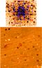 |
Fig. 1 Upper panel: the designed VISIR-Mosaic overlain on a 2MASS K-band image. The lower panel shows the central (F#7) VISIR 8.6 μm image. Red circles with |

Therefore, 47 Tuc still represents the key cluster to establish the luminosity extent of the mass-losing giants. Ideally one would like to re-examine this cluster with an appropriately high-resolution mid-IR instrument that allows a proper accounting of the higher central crowding conditions. Motivated by all the uncertainties still existing on the nature of the mass loss rate, we decided to exploit the superior capabilities of VISIR to re-examine the RGB stars of 47 Tuc with an appropriately high-resolution MIR instrument that allows a proper accounting of the higher central crowding conditions. In this paper we present 8.6 μm ground-based imaging data, which indeed achieve ~8 × better spatial resolution than that of Spitzer ( vs. 2 − 3′′).
In Sects. 2 and 3 we present the data reduction and calibration, in Sects. 4 and 5 we construct and analyse the combined optical-NIR-MIR colour − magnitude diagrams. Sections 6 presents the identified long-period variables and a spectroscopic study of the brightest AGB star. The conclusions are summarized in Sect. 7.
The journal of observations.
2. Observations and data reduction
2.1. The VISIR imaging data set
Our observations were obtained using the VLT spectrometer and imager for the MIR (VISIR, Lagage et al. 2004) currently located at the Cassegrain focus of UT3. VISIR provides diffraction-limited imaging at high sensitivity in the two mid infrared (MIR) atmospheric windows: the N-band between 8−13 μm and the Q-band between 16−24 μm. The observations were obtained with the VISIR PAH1 filter (λc = 8.59, Δλ = 0.42 μm). It is designed to avoid the telluric ozone band and provides a relatively high sensitivity.
Our programme [084.D-0721(A), P.I. Momany] was awarded 34 h. We used the  pixel scale for the imager, which yielded a field-of-view of
  × . Three observation blocks (OB) were dedicated to each of the 11 pointings, and each of these OBs had an effective integration time of 35 min, that is a total of ~1.75 h per pointing. These observations were carried out in service mode in the period between October 3, 2009 and January 30, 2010. Table 1 reports the J2000 right ascension and declination of the 11 VISIR pointings. Also reported are the offsets (in arc-seconds) from the cluster centre (as in Goldsbury et al. 2010) of each pointing and the dates at which the OBs were observed. Last column reports the number of stars found in each pointing.
As a result, the observations were spread over a four month period, obtained under various weather conditions. As for any ground-based mid-IR observations, the technique of chopping and nodding was used to enhance the detection of target stars over the background emission originating both from the sky and the telescope. The declination of 47 Tuc does not allow airmasses below 1.4 and around 90% of the obtained images had airmass between 1.4 and 1.8. The varying MIR weather conditions (i.e. water-vapor content, temperature, etc.) impacted heavily on the delivered quality of the data. In turn, the combination of the three OBs (of any given pointing) was not possible, even when these OBs were separated by only one day. Therefore we performed the photometric reduction (i.e. detection of point-sources and derivation of their aperture magnitudes) on the reduced image of each single OB separately.
The tested DAOPHOT (Stetson 1987) package was employed to perform the photometry on the reduced image for each OB. The FIND routine was set to a detection threshold of three times the background standard deviation estimated on a given image. In general, FIND detected about two to three times the number of the stars that one could identify by eye. A careful examination of the extra detections revealed that these are caused by abrupt fluctuations in the estimated background level or hot pixels. Indeed, even though we employed a relatively relaxed constraint, wherein a detection was considered real if found in at least two images, these extra detections did not survive the DAOMASTER matching process for a given field.
A powerful spurious-detections filtering process was performed when catalogues from at least two filters were combined. In this framework we decided to employ the astrometric/photometric HST/ACS mF606W, mF814W catalogue of 47 Tuc (Anderson et al. 2009, kindly provided by the author). This catalogue provided two advantages. The first was that the optical HST data were ~100% unaffected by photometric incompleteness around our VISIR data sampling. Indeed, the CMDs presented in Anderson et al. (2009) sampled ~8 mF606W magnitudes below the RGB tip, whereas our VISIR data address only the brightest ~2.0−2.5 mag. Moreover, the catalogue of Anderson et al. was based on the relatively red F606W and F814W filters, i.e. still sensitive to red sources with MIR-excess. The second advantage was that the ACS spatial resolution (pixel size of  ) is very close to that of our VISIR data. We therefore confidently used this HST catalogue in the VISIR point-source detection process. In other words, the ACS absolute astrometric positions were transformed to VISIR X, Y pixel coordinates, and a subset of this catalogue (V ≤ 13.0) was assumed to provide the detected point-sources.
In general, all objects visible in the VISIR N8.6 μm images had an optical HST counterpart (with V ≤ 13.0). This confirms that the use of the Anderson et al. HST catalogue did not introduce blue-filters selection effects in our final VISIR/ACS catalogue. There was one interesting case for which a visible VISIR target had a fainter optical counterpart, see Appendix A. Thus, this combined ACS/VISIR detection strategy provided us with the best possible elimination of spurious-detections.
Secondly,the respective catalogues were merged for each pointing to produce a single aperture magnitude catalogue. These magnitudes (see Table 2) were combined using the DAOPHOT/DAOMASTER task, which computed an intensity-weighted mean of the three aperture magnitudes in each field.
The upper panel in Fig. 1 displays the 2MASS K-band view of the core of 47 Tuc. Overlaid are the footprints of the 11 VISIR × pointings. Given the service mode nature of the programme and the necessity to ensure a common photometric scale for the single fields, the pointings were designed to overlap on bright stars (K ≤ 10 mag). Typically 2−4 such bright stars were shared among adjacent fields. A relative zero-point was computed from their magnitudes to bring all pointings on the photometric scale of pointing #7, which covered the cluster core. The lower panel of Fig. 1 displays the VISIR pipeline reduced image of a single 35-min OB. There is a one-to-one correspondence between all mF606W ≤ 13.0 stars from the Anderson et al. (2009) HST catalogue and VISIR detections. Although limited to a few cases, close stars (e.g., the two examples of stars falling within a  diameter circle) end up as blends in lower-resolution instruments. Lastly, adopting the HST determination of the cluster centre derived by Goldsbury et al. (2010), it is clear that our VISIR 8.6 μm imaging data covers the inner and most crowded core of the cluster.
2.2. VISIR spectroscopic data set
The VISIR N-band spectroscopy [Prog.60.A-9800(I)] consisted of two low-resolution (R ~ 300) setups with central wavelengths at 9.8 μm and 11.4 μm obtained with the  slit. These two setups were chosen to allow the coverage of the 10 μm silicate feature in a particularly bright AGB star (V8, see Sect. 6), which we observed to assess the quality of VISIR’s spectroscopic performance. To properly calibrate the data, the Standard VISIR Telluric HD 4815 was observed using the same setup. The data reduction was performed in two steps. First, the ESO/VISIR pipeline was used to extract the 2D frames of both the science target and the telluric. Later, we used the pipeline developed by Hönig et al. (2010), which is specifically designed to perform a proper background correction (including sky and periodic detector signals), beam extraction, 2D flux calibration and 1D spectrum extraction. The 2D spectrum of V8 and its calibrator HD 4810 showed very small FWHM variations. In particular, the 9.8 and 11.4 μm gratings of V8 showed a FWHM of
  and
and  , respectively. To recover ~ 96% of the flux in both setups, we employed an extraction aperture of
  and
and  for the 9.8 and 11.4 μm gratings, respectively. Lastly, we note that the two (9.8 and 11.4 μm) reduced spectrum of V8 showed almost perfect flux matching in the overlap wavelength region.
2.3. The HST catalogue
As explained above, the astrometric/photometric HST/ACS mF606W and mF814W catalogue of 47 Tuc (Anderson et al. 2009) was used as a reference catalogue for identifying the point sources in VISIR’s images. We refer the reader to Anderson et al.’s paper for details concerning the data reduction and calibrations. We complemented the Anderson et al. catalogue with independent measurements in mF336W, mF435W, mF606W and mF814W. This extends our final (mF606W, mF814W and N8.6 μm) catalogue with blue mF336W and mF435W measurements to avoid selection effects on high mass loss rate stars. The latter two photometric bands are based on reduction of ACS/Wide Field Channel (WFC) images from programme GO-10775, while mF435W is based on a single 10-s image from GO-9281. In both cases the photometric reduction and calibration of the ACS/WFC data was carried out using the software presented and described in detail in Anderson et al. (2008). The mF336W measurements were based on a 30-s exposure from GO-11729 obtained with the HST Wide Field Camera 3 (WFC3). This image was pre-reduced using the standard HST pipeline, while the fluxes were measured using a software based on the img2xym-WFI (Anderson et al. 2006) that will be presented in a separate paper (Anderson et al., in prep.).
2.4. The near-infrared catalogue
To sample the core of 47 Tuc in the NIR, we searched for available catalogues and archival ESO data. Unfortunately, given the extremely crowded conditions of the 47 Tuc core, observers tend to avoid this region. We used the excellent NIR JHKs catalogue of 47 Tuc of Salaris et al. (2007). This was based on high-resolution SOFI infrared images (pixel size of  ) obtained under excellent seeing conditions
  . However, the catalogue of Salaris et al. does not fully encompass the cluster core, but only the northern half. Moreover, the excellent seeing conditions resulted in saturation of the 47 Tuc upper RGB.
An archival SOFI [69.D-0604(A)] JHKs data set of 47 Tuc was also analysed. The data set was reduced following the standard methods presented in Momany et al. (2003). Unfortunately, this data set covered mainly the southern part around the cluster core, with a limited  overlap region with the Salaris et al. catalogue. The seeing on the averaged J- and Ks-band was
  and
and  , respectively, significantly worse than the data set of Salaris et al. (2007). The resulting NIR diagrams still showed saturation in the upper RGB and higher dispersion along the RGB. We therefore mainly used the Salaris et al. (2007) catalogue.
3. Calibration of the VISIR data
With the mosaicing strategy described above, the merged photometric catalogue of the 11 pointings was put on the photometric scale of pointing#7. The zero-point offsets were estimated from the stars in the overlapping regions. In this manner, the airmass and detector integration time (DIT) of pointing #7 could be used to calibrate the entire merged catalogue. We use the standard star HD 4815-K5III, observed just before the first OB of pointing #7, to flux-calibrate our data. The airmass of the HD 4815 was 1.569, while that of pointing #7 was 1.476. Although the calibration process is straightforward, ground-based MIR calibration can be tricky; we therefore provide a detailed presentation. First of all, we relied on the VISIR pipeline to deliver reduced images normalized to 1-second exposures. The instrumental magnitude of the standard star, which was observed in perpendicular CHOPPING/NODDING mode, was measured by the DAOPHOT/PHOT task. Four measurements were obtained, i.e. two measurements from each of the positive and negative beams. The averaged four measurements provided a standard deviation of less than ~2%. Before converting this average magnitude into a flux value, there remained two corrections to be applied: the aperture correction and the extinction.
3.1. Aperture correction
The first correction applied to the instrumental magnitudes is to correct for the loss of flux outside the adopted aperture radius: the so-called aperture-correction. This is usually made by estimating the magnitude difference between the employed aperture radius (2.5-pixels,  ) and those obtained at larger radii (out to 16-pixels,
  ). The aperture correction is measured at radii corresponding to a near constant magnitude difference, i.e. a plateau. In our case, the standard star aperture correction was quite significant: around 0.37 mag.
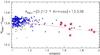 |
Fig. 2 Estimating the extinction coefficient for the |
3.2. Extinction coefficient
The second correction is that related to the airmass of the 47 Tuc VISIR observations. Given the cluster declination (and implied high airmass of ≥ 1.4), the extinction could not be ignored. Moreover, the extinction coefficient of the PAH1 filter (λc = 8.59 μm) has not been measured before.
For this purpose, we made use of an ESO-archival page1 to collect PAH1 standard star measurements for the past six years. Availing ourselves of the measured instrumental flux, and knowing the standard’s true flux (in Jansky, hereafter Jy), we show the results in Fig. 2. Only PAH1 with the -setup measurements are reported, and a 2.5σ clipping has been applied to the data-points for bins of airmass of 0.1. A least-square fit to σ-clipped data-points provided an extinction coefficient of 0.212 mag. This may seem relatively high (compared for example to the 0.05 mag for Ks-band), however, although there is a scarcity of published ground-based MIR extinction values, 0.212 was found to perfectly agree with technical tests2 made in a similar manner on TIMMI2 (previously mounted on the ESO/La Silla 3.6 m telescope).
In the specific case of HD 4815, the instrumental magnitude (minst.) corrected for airmass and aperture correction (apert. corr) corresponds to:  (1)
(1) (2)hence, the two corrections account for up to ~ 0.7 mag, making our photometric scale brighter.
3.3. Absolute fluxes and magnitudes
After correcting the standard star instrumental magnitude, we converted this into a flux value. This instrumental flux was divided by the standard star’s known flux (in Jansky units) to provide the conversion factor (ADU/Jy).
To derive the absolute calibration of the 47 Tuc PAH1 photometric catalogue, we first applied the aperture and extinction corrections (as performed for the standard star). Next, these corrected instrumental magnitudes were converted into fluxes and each star was divided by the conversion factor, obtained from the standard star. This basically converted our instrumental magnitudes into absolute flux values in Jy. The absolute flux (Fν, in units of Jansky) could then be converted into magnitudes on the (i) AB (Oke & Gunn 1983) photometric system:  (3)and (ii) the Merlin-N1 photometric system:
 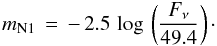 (4)The zero-point magnitude for the Merlin-N1 photometric scale (49.43 Jy) refers to an effective wavelength of 8.81 μm. This is slightly redder than the employed PAH1 filter (λc = 8.59, Δ λ = 0.42 μm). However, we note that there are no other ~ 8 μm filters in the UKIRT or in the Johnson systems (the closest being ~ 10.1 μm).
We caution that the AB and Merlin-N1 system differ systematically by a zero-point of 4.696 mag. For the remainder of this paper we will use the Merlin-N1 magnitude scale, and for brevity, refer to it as N8.6 μm.
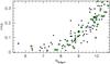 |
Fig. 3 Distribution of standard deviations (of stars with three photometric measurements) as a function of the N8.6 μm magnitude. Open circle highlight stars from pointing#7, while open triangles highlight those from pointing#3. |
3.4. Photometric errors
Ideally, photometric errors should be estimated from artificial star experiments by comparing the input/output magnitudes (e.g., Momany et al. 2008). However, for the majority of the 11 pointings, there were not enough detected stars to allow the construction of reliable point spread functions (PSF) necessary for the simulation/injection of artificial stars. On the other hand, each pointing had a total of three OBs4 and the standard deviation of these three measurements were used to trace the photometric errors in a given pointing. Figure 3 displays the distribution of the standard deviation as a function of the N8.6 μm magnitude for stars with three measurements. The distribution shows the expected increase of the rms as a function of magnitude. In particular, no significant rms variations were found among different pointings. The average photometric errors are listed in Table 2.
In addition to the photometric internal errors quantified in Fig. 3, we also have to consider the one caused by shifting of the photometric scales of the 10 pointings with respect to that of pointing#7. We quantified this additional error by first collecting the residuals around the average shift (as derived from the stars in the overlapping region of two adjacent fields), and subsequently estimating the rms of all the residuals. This turned out to be of the order of ~0.015 mag.
Lastly, we estimated the systematic uncertainty in calibrating the N8.6 μm data. The sources of uncertainty are those associated with the aperture-correction method and that from the derivation of the extinction coefficient in N8.6 μm. The aperture-correction uncertainty is of the order of 0.031 mag, estimated from the consistency of the value derived for the three single images of pointing#7. The uncertainty associated with the extinction coefficient derivation is of the order of 0.033 mag, estimated as the error on the slope of a least-square fit (as in Fig. 2). Overall, the total zero-point uncertainty, obtained from the quadratic sum of the above two factors is ~0.045 mag.
In Table 3 we report the VISIR N8.6 μm catalogue of the 47 Tuc central region, along with the mF606W and mF814W magnitudes (from Anderson et al. 2009), the mF336W and mF435W magnitudes (reduced in this paper), the J- and K-magnitudes (from Salaris et al. 2007), the flux value in Jansky and the known long-period variables (LPV) identification.
4. HST/VLT colour–magnitude diagrams
The combined ACS and VISIR N8.6 μm, (mF606W − N8.6 μm) colour − magnitude diagram of 47 Tuc core is presented in Fig. 4. The plotted error bars in both magnitude and colour are mainly driven by the photometric uncertainty in N8.6 μm, while those in the HST mF606W filter are lower than 0.002 mag. The brightest star at N8.6 μm = 5.595 is a known variable star (V8, see Sect. 6) with a total flux of 0.286 Jy, while the faintest reliable measurements reached (see Fig. 5) are for stars at N8.6 μm ≃ 10.0 (~0.005 Jy).
The CMD shows that we sampled the upper ~4 mag in N8.6 μm (~3 mag in mF814W filter) of the red giant branch of 47 Tuc. The horizontal branch level is expected at N8.6 μm ≃ 12.1, that is ~1.7 mag fainter than our photometric incompleteness level at around N8.6 μm ~ 10.4. Clearly, the VISIR ground-based observations did not compete with the deeper Spitzer CMDs.
The smoothly curved morphology of the upper RGB in the N8.6 μm, (mF606W − N8.6 μm) plane resembles that of optical mF814W, (mF606W − mF814W) diagrams published in Anderson et al. (2009). The N8.6 μm, (mF606W − N8.6 μm) CMD is not ideal to check for MIR-excess giants (see Fig. 8). Still, we note that there are no clear “outliers” (RGB or AGB) from the cluster mean RGB locus. Indeed, increasing photometric errors around fainter N8.6 μm magnitudes can confuse any RGB/AGB separation. To investigate this problem, we identified all AGB candidates using the optical mF814W, (mF606W − mF814W) HST diagram and examined their position on the optical/MIR diagram (see Fig. 5). Thanks to the HST photometric accuracy, AGB stars had a good (mF606W − mF814W) colour-separation from equally bright red giants and the group of stars belonging to the so-called early-AGB (at mF814W ~ 11.9) could be easily separated from RGB stars. Figure 5 shows that the selected AGB group, at most, overlap the RGB mean locus. In particular, for stars fainter than N8.6 μm ≃ 10.3 − 10.4, the photometric uncertainties and incompleteness appear strong enough to cause a sudden break in the slope of the RGB. This is clearly not a real feature, hence stars fainter than N8.6 μm ≃ 10.4 should not be considered.
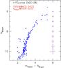 |
Fig. 4 Combined ACS and VISIR N8.6 μm, (mF606W − N8.6 μm) CMD of 47 Tuc. |
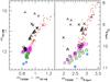 |
Fig. 5 Identification of AGB stars selected from the optical HST CMD on the combined N8.6 μm, (mF606W − N8.6 μm) diagram of 47 Tuc. The symbols in both panels trace particular (early and late) AGB groups as well as an arbitrary selection of the three faintest RGB groups. |
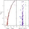 |
Fig. 6 Estimating the width of the RGB. The left-hand panel displays the derived RGB mean loci. Stars with (mF606W − N8.6 μm) ≤ 1.5 were excluded in this count. The right-hand panel displays the straightened RGB sequence, along which a bin of fixed-number of stars (5) is used to estimate the mean colour dispersion. For clarity, these are shifted to a mean colour of 3.0. |
4.1. The intrinsic width of the RGB
Related to the MIR-excess issue is the RGB intrinsic width, which apparently remains small all over the sampled ~3 N8.6 μm magnitudes. A quantitative estimate of the RGB width is obtained by straightening the RGB (with respect to a fiducial line or an isochrone), and, say, excluding any 2.5σ outliers (within a specified magnitude bin size). This is presented in Fig. 6. Excluding the upper two bins (relative to the AGB stars brighter than RGB tip) one appreciates how the thickness of the RGB is relatively uniform over ~3 mag along the RGB. The average RGB width turns out to be 0.095 ± 0.038, and no MIR-excess stars are detected. One has to apply a very strong 1.0σ clipping to identify outliers, and when this is applied, we note that the outliers are found mostly on the blue side of the RGB, therefore they are AGB candidates.
4.2. Isochrone fitting
The isochrone fitting is usually employed to derive/confirm the studied cluster distance, reddening and age. Our shallow data do not allow this level of analysis. Nevertheless, it provides an excellent test for ground-based calibration and, as we shall see, sheds lights on an interesting aspect of the RGB morphology. For the cluster distance and reddening we adopted the values derived in Carretta et al. (2000), namely (m − M)V = 13.55 and EB − V = 0.055. We adopted AV = 3.1 × EB − V, AF606W = 2.809 × EB − V, and a null AN8.6 μm. In Fig. 7 we display the optical-MIR diagram with a theoretical isochrone from the Padova library (Marigo et al. 2008)5. The isochrone was “coloured” with the N8.6 μm Vega magnitude using the VISIR PAH1 filter transmission curve (see Girardi et al. 2002, for details). The presented isochrone has an age of 12.59 Gyr and Z = 0.004 ([Fe/H] = − 0.67 as derived in Carretta et al. (2000) and Alves-Brito et al. (2005). Overall, the isochrone excellently agree with the RGB morphology.
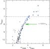 |
Fig. 7 Optical-MIR diagram along with an isochrone from the Padova library (Marigo et al. 2008). Adopted are an age of 12.59 Gyr, metallicity of Z = 0.004, distance of (m − M)° = 13.38 and reddening of EB − V = 0.055. The dashed line marks the RGB tip, while the horizontal branch level is expected at N8.6 μm ≃ 12.1. Open circles highlight the verified LPVs. The green arrow marks the ~1000 L⊙ luminosity level. |
For giants brighter than N8.6 μm ≃ 8.0 the observed RGB morphology seemingly deviate to redder colours than the isochrone loci. Interestingly, this magnitude level corresponds to luminosities of the order of ~1000 L⊙, suggested by McDonald et al. (2011a) to indicate the beginning of dusty mass loss for giants. This perfectly agrees with the AKARI study by Ita et al. (2007), who concluded that dust emission is mainly detected in AGB variables, although there are some variable stars with dust emission located below the RGB tip. Although this is very interesting, we note that we cannot firmly establish a connection between this small colour deviation and the onset of the dusty mass loss for giants below the RGB tip. Indeed, the stellar models of this cool Teff can be significantly affected by small errors in opacities and in the mixing length treatment. Moreover, one should keep in mind that the Kurucz spectra that were used to estimate the colour transformations may have additional sources of errors at this cool Teff. Consequently, the above factors caution against emphasizing this systematic deviation between the data and the isochrone.
In conclusion, the isochrone fitting to both the observed RGB colour and RGB-tip magnitude-level indicates an excellent theoretical handle of the unusual VISIR photometric system and well-calibrated data.
5. The Ks, (Ks – N8.6 μm) diagram
In the previous section we used our optical-MIR diagram to highlight the lack of RGB MIR-excess stars. However, it is quite difficult to draw any firm conclusion based solely on the basis of this diagram. Indeed, any MIR-excess emission would instead scatter the stars to brighter magnitudes and redder colours in a direction roughly parallel to the RGB morphology. This is quantitatively demonstrated in Fig. 8, where we plot the shift produced on the colour − magnitude diagram position of an upper RGB star as a function of the optical depth of the circumstellar dust shell for several O-rich dust mixtures that are included in the Marigo et al. (2008) isochrones. Figure 8 shows that the MIR excess can be best identified using the Ks, (Ks − N8.6 μm) plane (as in the original Origlia et al. 2007 paper) instead of the N8.6 μm, (mF606W − N8.6 μm) plane used in the previous section.
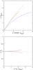 |
Fig. 8 Expected changes in colours and magnitudes of RGB stars caused by O-rich circumstellar dust shells for an optical depth at λ = 1 μm varying between 0 and 1, in the CMDs N8.6 μm vs. (mF606W − N8.6 μm) (upper panel) and Ks vs. (Ks − N8.6 μm) (lower panel). The different curves are for different dust compositions, namely the 100% AlOx (solid), 60% silicate + 40% AlOx (dotted), and 100% silicate (short-dashed) mixtures from Groenewegen (2006), and the silicates (long-dashed) from Bressan et al. (1998). |
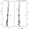 |
Fig. 9 Left-hand panel: Ks, (J − Ks) SOFI based diagram by Salaris et al. Light symbols display the entire catalogue, while open circles highlight stars with VISIR counterparts. The right-hand panel displays the SOFI VISIR matched Ks, (Ks − N8.6 μm) diagram. For comparison, the vertical line at (Ks − N8.6 μm) = 0.5 marks the location of the majority of MIR-excess stars seen in Fig. 2 of Origlia et al. (2007). |
To this end, we combined the optical/MIR catalogue of 47 Tuc with available NIR data and present the NIR/MIR diagrams in Fig. 9. The left panel displays the original Ks, (J − Ks) SOFI based diagram by Salaris et al. (2007). We remind the reader that this catalogue does not sample the upper RGB of 47 Tuc, because the excellent seeing conditions basically saturated the near RGB tip region. The right panel of Fig. 9 displays the SOFI and VISIR matched Ks, (Ks − N8.6 μm) diagram. This diagram shows that the RGB loci are perfectly vertical in the (Ks − N8.6 μm) plane, allowing a straightforward identification of possible MIR-excess stars. Evidently, one star shows a colour excess (see Appendix B). On the other hand, Fig. 2 of Origlia et al. (2007) shows a significant population with MIR-excess with (Ks − N8.6 μm) colours between 0.3 − 0.7. In conclusion, our NIR-MIR diagram shows that red giants at ~2 mag from the RGB tip and in an interval extending for ~2 more magnitudes do not show any particular signature of mass loss occurrence among the 47 Tuc red giants. We note that McDonald et al. (2011a) have performed a similar analysis (i.e. combining their re-reduced Spitzer data-sets with the Origlia et al. 2007 dusty sample) and found that almost half of the Origlia et al. MIR-excesses stars did not have counterparts in their re-reduction. In this regard, our higher-resolution ground-based NIR/MIR diagrams leave basically no space for the presence of a significant MIR-excess RGB population. This ultimately points towards the actual photometric reduction and intrinsic spatial resolution of the data as the primary cause of the detection of MIR-excess in 47 Tuc.
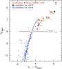 |
Fig. 10 Identified long-period variables in the N8.6 μm, (V° − N8.6 μm) plane. Certain identifications of the LPVs are plotted as red open circles, while uncertain identifications are plotted in different symbols, and only for the most plausible candidates. The V magnitudes of the LPVs were corrected for the known variability cycle, i.e. shifted to their average luminosity. The RGB tip is at N8.6 μm ≃ 7.0, while the suggested luminosity break is at N8.6 μm ≃ 8.0, corresponding to ~ 1000 L⊙. |
6. Long-period variables
Stellar pulsation is vital in the production of dust and mass loss (Ramdani & Jorissen 2001). Indeed, the luminosity range of mass-losing red giants is connected to the variable nature of these stars, and as already argued in McDonald et al. (2011a, and references therein), dust-producing stars tend to be exclusively variable, while variable stars tend to produce dust. We have identified the list of long-period variables presented and examined in the Lebzelter & Wood (2005, 2006) and Lebzelter et al. (2006). As displayed in Fig. 10, the majority of the LPVs found in our VISIR mosaic has certain identification (stars in open circles). In the particular case of LW13, we note that the low accuracy of the LPV coordinates in contrast to the high resolution provided by VISIR do not allow a definitive identification because it falls between two candidates stars. There is a very bright candidate (N8.6 μm = 6.333) at  located west, and a N8.6 μm = 7.233 located at east. For LW16 we have the opposite situation: the LPV is only
  away from a N8.6 μm = 8.224 candidate and
  from a brighter N8.6 μm = 7.501 candidate. Figure 10, clearly shows that all stars above the RGB tip (N8.6 μm ≃ 7.0) are AGB LPV. Moreover, and keeping in mind the particular case of LW16, one can infer that the occurrence of LPVs (in the current VISIR coverage) are present down to ~1 N8.6 μm magnitude below the RGB tip.
Following the referee’s suggestion, we also examined the mean optical V-magnitudes of the brightest and most variable AGB stars. Indeed, these can show quite significant V-variations (e.g. V8 varies up to ~1.7 mag) depending on the epoch of observation, which affects the star’s proper location in the colour-magnitude diagram. On the other hand, one can assume that the amplitude of the N8.6 μm variations would be failry small. For example, V8, the brightest of our AGB variables, is believed to have too small Ks-variations (Lebzelter & Wood 2006) for the phase of observation to be considered significant.
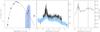 |
Fig. 11 Left-hand panel: SED of V8: black filled circles correspond to the observed photometry at mF435W, mF606W, mF814W (from the HST) J, H, Ks (from 2MASS), N8.6 μm (from VISIR), plus 9 and 18 μm from AKARI. The dotted dashed black line is the best-fitting black-body with a temperature of of 2900 K. The VISIR N8.6 μm filter transmission curve is shown in red, while that of AKARI 9 μm is shown in shaded blue. The middle panel displays a comparison of the VISIR (solid black line) and IRS (dashed blue line) spectra. The shaded areas highlight the flux calibration uncertainties estimated for the two spectra. The right-hand panel shows the MIR excess for V8 (continuum subtracted spectrum) where the features at 9.7 and 11.5 μm are highlighted with vertical dotted lines. |
The majority of monitoring studies that address these bright AGB stars in 47 Tuc are ground-based (e.g., Lebzelter & Wood 2006; Weldrake et al. 2004). We therefore converted the HST/ACS mF606W magnitudes into Johnson-V, following the procedure outlined in Saviane et al. (2008). It employs the stars dereddened mF606W magnitudes and mF606W − mF814W colours and the transformation coefficients listed in Table 14 of Sirianni et al. (2005). The resulting V° and I° magnitudes were compared to the 47 Tuc ground-based catalogue presented in Alves-Brito et al. (2005), which excellently agreed. The mean V-luminosities were then derived using the Lebzelter & Wood (2005) and Lebzelter et al. (2006) light curves, which we compared with the HST’s (JD = 2 453 807.6 epoch) newly converted V-magnitudes.
With the exception of V20 (at V° = 12.623 is observed at its minimum phase) the remaining LPVs tend (in different measures) towards having redder (V° − N8.6 μm) colours, which additinally support their MIR-excess. In Sect. 4.2 we cautioned against emphasizing the small colour deviation between the stars and the isochrone, in correspondence of the ~1000 L⊙ luminosity level. We note, however, that correcting for the optical V mean magnitudes would increase this off-isochrone colour deviation (starting at N8.6 μm ~ 8.0) even more. Overall, Fig. 10 shows that dusty mass loss: (i) is triggered at the ~ 1000 L⊙ luminosity level; (ii) is strongly associated with the RGB/AGB pulsation properties; (iii) is relatively weak along the RGB; and lastly (iv) is not an episodic process.
In Fig. 11 we focus our attention on the brightest of these LPVs in our sample (V8) and complement the derived N8.6 μm flux with a VISIR 8 − 13 μm low-resolution (R ~ 350) spectrum (see van Loon et al. 2006, for similar studies). According to the study of Lebzelter & Wood (2006), V8 is a ~100-day period fundamental-mode radial pulsator. The middle panel of Fig. 11 displays the VISIR V8 spectrum (black solid line) compared to the lower-resolution (R ~ 100) Spitzer/IRS spectrum (light blue line) presented in Lebzelter et al. (2006). The shaded areas highlight the flux calibration uncertainties estimated for both spectra. In particular, for the IRS spectrum we made use of the pipeline reduction, which has an uncertainty of ~10%, in comparison to ~5% uncertainty for the more detailed reduction presented in Lebzelter et al. (2006). Interestingly, the main dust features in the VISIR and IRS spectra are very similar. There is a visible flux level difference between the VISIR and IRS spectra, but we note that this is within the estimated errors, as shown by the shaded areas.
For a better characterization of its MIR excess, we compiled a fairly complete SED of V8 using photometric data from HST, 2MASS, VISIR, and AKARI6, covering the range from near-UV to the MIR. The best-fit temperature (dotted-dashed line in the left panel of Fig. 11) is found to be 2900 K, and this temperature was subsequently used to model the continuum. At longer wavelength, we note that the VISIR N8.6 μm data point shows a better match with respect to the AKARI 9 μm data point. The difference is probably caused by the slightly “bluer” and narrower VISIR PAH1 filter, which make it less sensitive to dust emission, while the AKARI data are more sensitive to the silicate feature.
To better characterize the silicate feature, we employed the previously fitted black-body as continuum and subtracted it from the dusty VISIR spectrum of V8. We note that because we are in the Rayleigh-Jeans domain, the difference between subtracting a black-body of this temperature and one within ± 1000 K should be negligible. The right panel finally displays the VISIR V8 continuum-subtracted spectrum. The dominant dust features are expected at around 9.7, 11.5 and 13 μm. The VISIR V8 spectrum is limited to 12.5 μm; however, the 13 μm feature was detected in the studies of Lebzelter et al. (2006) and McDonald et al. (2011b). As discussed in Lebzelter et al. (2006), the dust (9.7, 11.5 and 13 μm) features show different strength in correlation with the star’s position along the AGB. At the highest luminosities, as is the case for V8, the 9.7 μm feature is expected to dominate those at the remaining two wavelengths. This is clearly visible in the right panel of Fig. 11. In particular, the ~10 μm feature of V8 consists of a broad feature with an emerging 9.7 μm silicate bump. The feature at 11.5 μm is, as expected, weaker than that at 9.7 μm. Although there is no general consensus (see Lebzelter et al. 2006), it is believed that the feature at 11.5 μm is caused by amorphous aluminum oxide Al2O3 (McDonald et al. 2011b).
The strong 9.7 μm silicate bump observed in the VISIR spectrum was not detected in the only other ground-based MIR spectrum of V8 presented by van Loon et al. (2006). The absence of this feature has led Lebzelter et al. (2006) to suggest possible phase-dependent background impacting the van Loon et al. (2006) TIMMI2 spectrum. However, the detection of the feature in our ground-based VISIR spectrum clearly point towards a higher-sensitivity provided by the VISIR/VLT (8-m class telescope) combination with respect to that of TIMMI2 and ESO/3.6-m telescope.
The V8 9.7 μm silicate feature places V8 as a broad+sil AGB in the dust classification scheme of Speck et al. (2000). Interestingly, however, and as evident from the spectrum presented in Lebzelter et al. (2006) and McDonald et al. (2011b), V8 displays the dust features at all three wavelengths. This adds some confusion to its classification. Indeed, the 13 μm feature (very similar to that of SAO 37673) is commonly found in non-Mira semi-regular variables according to Speck et al. (2000). On the other hand, following Sloan et al. (2010), the same 13 μm feature is detected in Miras. This agrees with the results presented in Lebzelter & Wood (2005), showing that the V8 velocity curve resembles those of typical Miras found in the solar neighbourhood. Yet again, the V-band amplitude of V8 of ~1.7 mag. (Arp et al. 1963) is smaller than the nominal 2.5 mag value used in the classical definition of Miras. In conclusion, a proper classification of V8 is intrinsically difficult. Future monitoring of the V8 (and other dusty AGB stars) silicate feature is required to better characterize the relation between dust production and pulsation modes.
7. Conclusions
The Spitzer-based Origlia et al. (2007) study of 47 Tuc has triggered a wave of interest concerning the process of mass loss in red giants. Their results showed that a significant fraction of the 47 Tuc RGB population has MIR-excess. In particular, this MIR-excess was affecting red giants already at the horizontal branch level. This initiated a very interesting debate on whether the Spitzer results were induced by its low spatial resolution and the extreme crowding of the cluster core.
The VISIR high-resolution capabilities have allowed us to address this debate with an independent data set that provided the cleanest possible catalogue to test the Spitzer-based results. We have complemented our VISIR 8.6 μm data with near-UV, optical and NIR photometry to construct colour-magnitude diagrams best-suited to detect the MIR excess along the RGB. From the analysis of these diagrams and sampling down to about ~3 mag below the RGB tip, we found no evidence for the presence of dusty circumstellar envelopes around 47 Tuc RGB stars. In particular, down to this magnitude level, all stars (but one) are consistent with no MIR-excess. Fainter than N8.6 μm ≃ 10 (i.e. ≥ 4.0 mag below the RGB tip) photometric uncertainties do not allow any firm conclusion, but the data are still consistent with the null-hypothesis. In conclusion, we do not confirm the results of Origlia et al. (2007). Instead, we show that RGB stars are not affected by dusty mass loss except those within ~1 mag range from the RGB tip.
There is an observed break at N8.6 μm ≃ 8.0 that signals the onset of a colour deviation between the stars and the theoretical isochrone. Uncertainties in the colour transformations and opacity and mixing length treatment all caution against emphasizing this colour deviation between the data and the isochrone. Nevertheless, it is interesting to note that this luminosity level corresponds to ~1000 L⊙, which was suggested by independent determinations (McDonald et al. 2011b) to sign the onset of the dusty mass loss.
Finally, the VISIR high-resolution capabilities that were demonstrated in this paper will allow us to plan other studies of the brightest giants in Galactic globular clusters, spanning a wide range in metallicity. This and related projects will surely benefit from the forthcoming ESO/VISIR detector upgrade, which is planned for October 2012.
Online material
The VISIR N8.6 μm catalogue of the 47 Tuc central region.
Appendix A: Peculiar object #1
In general, all objects reported in Table 3 were visible by eye in the VISIR images, and had an optical HST counterpart (with mF606W ≤ 13.0). One exception is target ID#98781, which showed an irregular shape in the VISIR N8.6 μm images and had an HST counterpart (within a 1-pixel matching radius) that is fainter than mF606W ~ 13.0. This target fell in field#3 at (RA, Dec)J2000 = (6.0323672, − 72.0677501) and had mF606W, mF814W, N8.6 μm, J-, and K-magnitudes of 16.100, 15.423, 8.022, 14.809 and 14.225, respectively. The irregular shape of the target hinted at a background galaxy, and this was confirmed after building the SED of that source (see Fig. A.1). The SED fitting was performed with the Multi-wavelength Analysis of Galaxy Physical Properties (MAGPHYS code) presented in Cunha et al. (2008). This indicates a z ~ 0.3 redshift galaxy with a total mass of ~2 × 10¹¹ M⊙ and a quite significant star-formation rate of ~150 M⊙/yr.
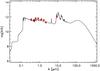 |
Fig. A.1 Red symbols show the SED of the peculiar VISIR target (ID#98781) with faint HST counterpart. The black line reports the best fit obtained with the MAGPHYS code, corresponding to a z ~ 0.3 redshift galaxy. |
Appendix B: Peculiar object #2
Another peculiar red target (ID#89862) is that seen in Fig. 9. Located at (RA, Dec)J2000 = (6.06149167, − 72.07903611), it has mF606W, mF814W, N8.6 μm, J-, and K-magnitudes of 11.120, 9.765, 7.052, 10.953 and 9.680, respectively. Indeed, it is V19 as reported in Table 3. In the optical mF814W, (mF606W − mF814W) colour − magnitude diagram, this star shows up as a bright AGB candidate, located to the left side of the RGB mean loci. On the other hand, and in the N8.6 μm vs. (mF606W − N8.6 μm) diagram (see Fig. 10), it is located very close to RGB tip. Basically, the near-infrared J- and K-magnitudes (as reported in the Salaris et al. catalogue) show a significant colour excess. We repeated the VISIR/HST/SOFI coordinate matching and visually inspected the location of this star in the images. This test confirmed our initial identification, and showed no particular indication of possible blending or mismatch caused by a faint unresolved companion. Moreover, the analysis on the optical V mean magnitude of this variable did not indicate significant variations.
In conclusion, the Salaris et al. (2007) photometry of V19 shows a rather fainter than expected J- and K-magnitudes. Indeed, the 2MASS J- and K-photometry of V19 (8.695 and 7.567, respectively) is ~2 mag brighter than that reported in Salaris et al. (2007). After excluding a possible coordinate mismatch, we caution that the Salaris et al. (2007) catalogue (see Sect. 2.4) suffered photometric saturation around K ≃ 8.0. This throws some doubt on the Salaris et al. (2007) photometry of V19 and, consequently, on its position in the Fig. 9. Lastly, this variable will be subject of a future investigation.
The VISIR service mode observations adopt a reference flux level (expressed in terms of mJy/hour) that is measured on MIR standard stars observed either before or after the science OB. There were few OBs (of the order of 1−2 per pointing) that exceeded the reference flux values and these OBs were excluded from our analysis.
The isochrones are available at http://stev.oapd.inaf.it/cmd
AKARI-FIS Bright Source Catalogue Release note Version 1.0 Yamamura, I., Makiuti, S., Ikeda, N., Fukuda, Y., Oyabu, S., Koga, T., White, G. J. 2010.
Acknowledgments
We thank the anonymous referee for his/her comments that improved the presentation of the paper. We also thank Jay Anderson and Maurizio Salaris for providing us with the HST and NTT catalogues, respectively. Caroline Foster and Magaretha Pretorius are acknowledged for a careful reading of the manuscript. L.G. and A.B. acknowledge partial support from contract ASI-INAF I/009/10/0. This research is based on observations with AKARI, a JAXA project with the participation of ESA.
References
- Alves-Brito, A., Barbuy, B., Ortolani, S., et al. 2005, A&A, 435, 657 [NASA ADS] [CrossRef] [EDP Sciences] [Google Scholar]
- Anderson, J., Bedin, L. R., Piotto, G., Yadav, R. S., & Bellini, A. 2006, A&A, 454, 1029 [NASA ADS] [CrossRef] [EDP Sciences] [Google Scholar]
- Anderson, J., King, I. R., Richer, H. B., et al. 2008, AJ, 135, 2114 [NASA ADS] [CrossRef] [Google Scholar]
- Anderson, J., Piotto, G., King, I. R., Bedin, L. R., & Guhathakurta, P. 2009, ApJ, 697, L58 [NASA ADS] [CrossRef] [Google Scholar]
- Arp, H., Brueckel, F., & Lourens, J. V. B. 1963, ApJ, 137, 228 [NASA ADS] [CrossRef] [Google Scholar]
- Boyer, M. L., McDonald, I., Loon, J. T., et al. 2008, AJ, 135, 1395 [NASA ADS] [CrossRef] [Google Scholar]
- Boyer, M. L., van Loon, J. Th., McDonald, I., et al. 2010, ApJ, 711, L99 [NASA ADS] [CrossRef] [Google Scholar]
- Bressan, A., Granato, G. L., & Silva, L. 1998, A&A, 332, 135 [NASA ADS] [Google Scholar]
- Caloi, V., & D’Antona, F. 2008, ApJ, 673, 847 [NASA ADS] [CrossRef] [Google Scholar]
- Carretta, E., Gratton, R. G., Clementini, G., & Fusi Pecci, F. 2000, ApJ, 533, 215 [NASA ADS] [CrossRef] [Google Scholar]
- Carretta, E., Bragaglia, A., Gratton, R. G., et al. 2009, A&A, 505, 117 [NASA ADS] [CrossRef] [EDP Sciences] [Google Scholar]
- Cunha, E., Charlot, S., & Elbaz, F. 2008, MNRAS, 388, 1595 [NASA ADS] [CrossRef] [Google Scholar]
- D’Antona, F., & Caloi, V. 2008, MNRAS, 390, 693 [NASA ADS] [CrossRef] [Google Scholar]
- Fagotto, F., Bressan, A., Bertelli, G., & Chiosi, C. 1994, A&AS, 105, 29 [NASA ADS] [Google Scholar]
- Girardi, L., Bertelli, G., Bressan, A., et al. 2002, A&A, 391, 195 [NASA ADS] [CrossRef] [EDP Sciences] [Google Scholar]
- Goldsbury, R., Richer, H. B., Anderson, J., et al. 2010, AJ, 140, 1830 [NASA ADS] [CrossRef] [Google Scholar]
- Groenewegen, M. A. T. 2006, A&A, 448, 181 [NASA ADS] [CrossRef] [EDP Sciences] [Google Scholar]
- Hönig, S. F., Kishimoto, M., Gandhi, P., et al. 2010, A&A, 515, A23 [NASA ADS] [CrossRef] [EDP Sciences] [Google Scholar]
- Ita, Y., Tanabé, T., Matsunaga, N., et al. 2007, PASJ, 59, 437 [Google Scholar]
- Lagage, P. O., Pel, J. W., Authier, M., et al. 2004, The Messenger, 117, 12 [NASA ADS] [Google Scholar]
- Lebzelter, T., & Wood, P. R. 2005, A&A, 441, 1117 [NASA ADS] [CrossRef] [EDP Sciences] [Google Scholar]
- Lebzelter, T., & Wood, P. R. 2006, Mem. Soc. Astron. Ital., 77, 55 [NASA ADS] [Google Scholar]
- Lebzelter, T., Posch, T., Hinkle, K., Wood, P. R., & Bouwman, J. 2006, ApJ, 653, L145 [NASA ADS] [CrossRef] [Google Scholar]
- Marigo, P., Girardi, L., Bressan, A., et al. 2008, A&A, 482, 883 [NASA ADS] [CrossRef] [EDP Sciences] [Google Scholar]
- McDonald, I., van Loon, J. T., Decin, L., et al. 2009, MNRAS, 394, 831 [NASA ADS] [CrossRef] [Google Scholar]
- McDonald, I., Boyer, M. L., van Loon, J. Th., et al. 2011a, ApJS, 193, 23 [NASA ADS] [CrossRef] [Google Scholar]
- McDonald, I., Boyer, M. L., van Loon, J. T., & Zijlstra, A. A. 2011b, ApJ, 730, 71 [NASA ADS] [CrossRef] [Google Scholar]
- Momany, Y., Ortolani, S., Held, E. V., et al. 2003, A&A, 402, 607 [NASA ADS] [CrossRef] [EDP Sciences] [Google Scholar]
- Momany, Y., Ortolani, S., Bonatto, C., Bica, E., & Barbuy, B. 2008, MNRAS, 391, 1650 [NASA ADS] [CrossRef] [Google Scholar]
- Oke, J. B., & Gunn, J. E. 1983, ApJ, 266, 713 [NASA ADS] [CrossRef] [Google Scholar]
- Origlia, L., Ferraro, F. R., Fusi Pecci, F., & Rood, R. T. 2002, ApJ, 571, 458 [NASA ADS] [CrossRef] [Google Scholar]
- Origlia, L., Rood, R. T., Fabbri, S., et al. 2007, ApJ, 667, L85 [NASA ADS] [CrossRef] [Google Scholar]
- Origlia, L., Rood, R. T., Fabbri, S., et al. 2010, ApJ, 718, 522 [NASA ADS] [CrossRef] [Google Scholar]
- Piotto, G., Villanova, S., Bedin, L. R., et al. 2005, ApJ, 621, 777 [NASA ADS] [CrossRef] [Google Scholar]
- Ramdani, A., & Jorissen, A. 2001, A&A, 372, 85 [NASA ADS] [CrossRef] [EDP Sciences] [Google Scholar]
- Reimers, D. 1975a, in Problems in Stellar Atmospheres and Envelopes, ed. B. Baschek, W. H. Kegel, & G. Traving (Berlin: Springer), 229 [Google Scholar]
- Reimers, D. 1975b, Mem. Soc. R. Sci. Liege, 8, 369 [NASA ADS] [Google Scholar]
- Renzini, A. 2008, MNRAS, 391, 354 [NASA ADS] [CrossRef] [Google Scholar]
- Rood, R. T. 1973, ApJ, 184, 815 [NASA ADS] [CrossRef] [Google Scholar]
- Salaris, M., Held, E. V., Ortolani, S., Gullieuszik, M., & Momany, Y. 2007, A&A, 476, 243 [NASA ADS] [CrossRef] [EDP Sciences] [Google Scholar]
- Saviane, I., Momany, Y., da Costa, G. S., Rich, R. M., & Hibbard, J. E. 2008, ApJ, 678, 179 [NASA ADS] [CrossRef] [Google Scholar]
- Skrutskie, M. F., Cutri, R. M., Stiening, R., et al. 2006, AJ, 131, 1163 [NASA ADS] [CrossRef] [Google Scholar]
- Sirianni, M., Jee, M. J., Benítez, N., et al. 2005, PASP, 117, 1049 [NASA ADS] [CrossRef] [Google Scholar]
- Sloan, G. C., Matsunaga, N., Matsuura, M., et al. 2010, AJ, 719, 1274 [Google Scholar]
- Speck, A. K., Barlow, M. J., Sylvester, R. J., & Hofmeister, A. M. 2000, A&AS, 146, 437 [NASA ADS] [CrossRef] [EDP Sciences] [Google Scholar]
- Stetson, P. B. 1987, PASP, 99, 191 [NASA ADS] [CrossRef] [Google Scholar]
- van Loon, J. T., McDonald, I., Oliveira, J. M., et al. 2006, A&A, 450, 339 [NASA ADS] [CrossRef] [EDP Sciences] [Google Scholar]
- van Loon, J. T., Boyer, M. L., & McDonald, I. 2008, ApJ, 680, L49 [NASA ADS] [CrossRef] [Google Scholar]
- Weldrake, D. T. F., Sackett, P. D., Bridges, T. J., & Freeman, K. C. 2004, AJ, 128, 736 [NASA ADS] [CrossRef] [Google Scholar]
All Tables
All Figures
|
Fig. 1 Upper panel: the designed VISIR-Mosaic overlain on a 2MASS K-band image. The lower panel shows the central (F#7) VISIR 8.6 μm image. Red circles with |
| In the text | |
|
Fig. 2 Estimating the extinction coefficient for the |
| In the text | |
|
Fig. 3 Distribution of standard deviations (of stars with three photometric measurements) as a function of the N8.6 μm magnitude. Open circle highlight stars from pointing#7, while open triangles highlight those from pointing#3. |
| In the text | |
|
Fig. 4 Combined ACS and VISIR N8.6 μm, (mF606W − N8.6 μm) CMD of 47 Tuc. |
| In the text | |
|
Fig. 5 Identification of AGB stars selected from the optical HST CMD on the combined N8.6 μm, (mF606W − N8.6 μm) diagram of 47 Tuc. The symbols in both panels trace particular (early and late) AGB groups as well as an arbitrary selection of the three faintest RGB groups. |
| In the text | |
|
Fig. 6 Estimating the width of the RGB. The left-hand panel displays the derived RGB mean loci. Stars with (mF606W − N8.6 μm) ≤ 1.5 were excluded in this count. The right-hand panel displays the straightened RGB sequence, along which a bin of fixed-number of stars (5) is used to estimate the mean colour dispersion. For clarity, these are shifted to a mean colour of 3.0. |
| In the text | |
|
Fig. 7 Optical-MIR diagram along with an isochrone from the Padova library (Marigo et al. 2008). Adopted are an age of 12.59 Gyr, metallicity of Z = 0.004, distance of (m − M)° = 13.38 and reddening of EB − V = 0.055. The dashed line marks the RGB tip, while the horizontal branch level is expected at N8.6 μm ≃ 12.1. Open circles highlight the verified LPVs. The green arrow marks the ~1000 L⊙ luminosity level. |
| In the text | |
|
Fig. 8 Expected changes in colours and magnitudes of RGB stars caused by O-rich circumstellar dust shells for an optical depth at λ = 1 μm varying between 0 and 1, in the CMDs N8.6 μm vs. (mF606W − N8.6 μm) (upper panel) and Ks vs. (Ks − N8.6 μm) (lower panel). The different curves are for different dust compositions, namely the 100% AlOx (solid), 60% silicate + 40% AlOx (dotted), and 100% silicate (short-dashed) mixtures from Groenewegen (2006), and the silicates (long-dashed) from Bressan et al. (1998). |
| In the text | |
|
Fig. 9 Left-hand panel: Ks, (J − Ks) SOFI based diagram by Salaris et al. Light symbols display the entire catalogue, while open circles highlight stars with VISIR counterparts. The right-hand panel displays the SOFI VISIR matched Ks, (Ks − N8.6 μm) diagram. For comparison, the vertical line at (Ks − N8.6 μm) = 0.5 marks the location of the majority of MIR-excess stars seen in Fig. 2 of Origlia et al. (2007). |
| In the text | |
|
Fig. 10 Identified long-period variables in the N8.6 μm, (V° − N8.6 μm) plane. Certain identifications of the LPVs are plotted as red open circles, while uncertain identifications are plotted in different symbols, and only for the most plausible candidates. The V magnitudes of the LPVs were corrected for the known variability cycle, i.e. shifted to their average luminosity. The RGB tip is at N8.6 μm ≃ 7.0, while the suggested luminosity break is at N8.6 μm ≃ 8.0, corresponding to ~ 1000 L⊙. |
| In the text | |
|
Fig. 11 Left-hand panel: SED of V8: black filled circles correspond to the observed photometry at mF435W, mF606W, mF814W (from the HST) J, H, Ks (from 2MASS), N8.6 μm (from VISIR), plus 9 and 18 μm from AKARI. The dotted dashed black line is the best-fitting black-body with a temperature of of 2900 K. The VISIR N8.6 μm filter transmission curve is shown in red, while that of AKARI 9 μm is shown in shaded blue. The middle panel displays a comparison of the VISIR (solid black line) and IRS (dashed blue line) spectra. The shaded areas highlight the flux calibration uncertainties estimated for the two spectra. The right-hand panel shows the MIR excess for V8 (continuum subtracted spectrum) where the features at 9.7 and 11.5 μm are highlighted with vertical dotted lines. |
| In the text | |
|
Fig. A.1 Red symbols show the SED of the peculiar VISIR target (ID#98781) with faint HST counterpart. The black line reports the best fit obtained with the MAGPHYS code, corresponding to a z ~ 0.3 redshift galaxy. |
| In the text | |
Current usage metrics show cumulative count of Article Views (full-text article views including HTML views, PDF and ePub downloads, according to the available data) and Abstracts Views on Vision4Press platform.
Data correspond to usage on the plateform after 2015. The current usage metrics is available 48-96 hours after online publication and is updated daily on week days.
Initial download of the metrics may take a while.