| Issue |
A&A
Volume 536, December 2011
|
|
|---|---|---|
| Article Number | A28 | |
| Number of page(s) | 12 | |
| Section | Stellar structure and evolution | |
| DOI | https://doi.org/10.1051/0004-6361/201117739 | |
| Published online | 05 December 2011 | |
Thermohaline instability and rotation-induced mixing
II. Yields of 3He for low- and intermediate-mass stars
1
Geneva Observatory, University of Geneva, Chemin des Mailettes 51, 1290 Versoix, Switzerland
e-mail: This email address is being protected from spambots. You need JavaScript enabled to view it.
2
IRAP, UMR 5277 CNRS and Université de Toulouse, 14, Av. E. Belin, 31400 Toulouse, France
Received: 21 July 2011
Accepted: 13 September 2011
Abstract
Context. The 3He content of Galactic HII regions is very close to that of the Sun and the solar system, and only slightly higher than the primordial 3He abundance as predicted by the standard Big Bang nucleosynthesis. However, the classical theory of stellar evolution predicts a high production of 3He by low-mass stars, implying a strong increase of 3He with time in the Galaxy. This is the well-known “3He problem”.
Aims. We study the effects of thermohaline and rotation-induced mixings on the production and destruction of 3He over the lifetime of low- and intermediate-mass stars at various metallicities.
Methods. We compute stellar evolutionary models in the mass range 1 to 6 M⊙ for four metallicities, taking into account thermohaline instability and rotation-induced mixing. For the thermohaline diffusivity we use the prescription based on the linear stability analysis, which reproduces red giant branch (RGB) abundance patterns at all metallicities. Rotation-induced mixing is treated taking into account meridional circulation and shear turbulence. We discuss the effects of these processes on internal and surface abundances of 3He and on the net yields.
Results. Over the whole mass and metallicity range investigated, rotation-induced mixing lowers the 3He production, as well as the upper mass limit at which stars destroy 3He. For low-mass stars, thermohaline mixing occuring beyond the RGB bump is the dominant process in strongly reducing the net 3He yield compared to standard computations. Yet these stars remain net 3He producers.
Conclusions. Overall, the net 3He yields are strongly reduced compared to the standard framework predictions.
Key words: stars: evolution / stars: abundances / stars: low-mass / stars: rotation / Galaxy: abundances / primordial nucleosynthesis
© ESO, 2011
1. Introduction
The classical theory of stellar evolution predicts a very simple Galactic destiny for 3He, dominated by the production of this isotope during the Big Bang nucleosynthesis (BBN) and in stars with initial masses lower than ~3 M⊙. In these objects, 3He is produced first through D-processing on the pre-main sequence and then through the pp-chain on the main sequence. This fresh 3He is then engulfed in the stellar convective envelope during the so-called first dredge-up when the stars move towards the red giant branch (Iben 1967). According to classical modelling1, it survives the following stellar evolution phases before it is released in the interstellar matter through stellar wind and planetary nebula ejection (Rood et al. 1976; Vassiliadis & Wood 1993; Dearborn et al. 1996; Weiss et al. 1996; Forestini & Charbonnel 1997). Two planetary nebulae, namely NGC 3242 and J320, whose estimated initial masses were slightly higher than that of the Sun, have been found to “behave classically”: they are presently expelling freshly synthesized elements among which is 3He with the amount predicted by classical stellar models (Balser et al. 1997, 1999, 2006; Galli et al. 1997).
As a consequence, one expects a steep increase of 3He with time in the Galaxy with respect to its primordial abundance (see e.g. Wilson & Rood 1994), this latest quantity being well constrained through accurate determination of the baryon density of the Universe by recent cosmic microwave background experiments, most particularly from WMAP (Spergel et al. 2003; Dunkley et al. 2009), which has led to an unprecedented precision on the yields of standard BBN (Coc et al. 2004; Cyburt et al. 2008). Galactic HII regions in particular should be highly enriched in 3He because their matter content chronicles the result of billion years of chemical evolution since the Milky Way formation. Additionally, the present 3He/H abundance ratio is expected to be higher in the central regions of the Galaxy, where there has been more substantial stellar processing than in the solar neighbourhood. However, the 3He abundance in HII regions that sample a large volume of the Galactic disk is found to be relatively homogeneous (Rood et al. 1979; Balser et al. 1994, 1999; Bania et al. 1997, 2002, 2010); its average value is similar to that of the Sun at the epoch of its formation (for references see Geiss & Gloeckler 2010), and only slightly higher than the WMAP+SBBN primordial abundance2. No observational evidence is therefore found for the strong enrichment of this element in the Galactic history, contrary to expectations from all chemical evolution models that take into account 3He yields from classical stellar models (e.g. Galli et al. 1995; Olive et al. 1995; Tosi 1996).
This is the well-known “3He problem” that could be solved if only ~10% or less of all low-mass stars were actually releasing 3He, as predicted by the classical stellar theory (Tosi 1998, 2000; Palla et al. 2000; Chiappini et al. 2002; Romano et al. 2003), among which are NGC 3242 and J320. In other words, the lack of increase of the Galactic 3He abundance can be accounted for if most ( ≥ 90%) low-mass stars consume most of the 3He they produce during the main sequence before it can be released into the interstellar medium. This calls for a physical process that is ignored by the classical theory of stellar evolution, but whose spectroscopic signatures have been revealed long ago at the surface of relatively bright low-mass red giants. In particular, one observes a sudden drop of the surface 12C/13C ratio as low-mass stars evolve beyond the so-called luminosity bump on the red giant branch (RGB) well after the end of the first dredge-up (Gilroy 1989; Gilroy & Brown 1991; Charbonnel 1994; Charbonnel et al. 1998; Gratton et al. 2000; Tautvaišiene et al. 2000, 2005; Shetrone 2003; Pilachowski et al. 2003; Spite et al. 2006; Recio-Blanco & de Laverny 2007; Charbonnel & Lagarde 2010b). This behaviour, which is not predicted by standard stellar modelling, appears to be almost universal. Indeed, about 96% of all low-mass bright red giant stars exhibit unexpectedly low 12C/13C, regardless of whether they belong to the field, to open or globular clusters (Charbonnel & Do Nascimento 1998), or even to external galaxies (Smith et al. 2002; Geisler et al. 2005).
This high number satisfies the Galactic requirements for the evolution of the 3He abundance because the mechanism responsible for the low values of 12C/13C is also expected to lead to the depletion of 3He by a large factor in the stellar envelopes, as initially suggested by Rood et al. (1984; see also Charbonnel 1995; Hogan 1995; Sackmann & Boothroyd 1999; Eggleton et al. 2006). This correlation was recently confirmed by Charbonnel & Zahn (2007b) and Eggleton et al. (2008), who included the transport of chemicals caused by thermohaline mixing in stellar models (see also Stancliffe et al. 2009; Charbonnel & Lagarde 2010a). In red giant stars, this double diffusive instability (also called “fingering convection”), is induced by the mean molecular weight inversion created by the 3He(3He, 2p)4He reaction in the region between the hydrogen-burning shell and the convective envelope (Charbonnel & Zahn 2007b)3. It sets in naturally as soon as stars reach the so-called luminosity bump on the RGB. However, and importantly in the 3He context, Charbonnel & Zahn (2007a) proposed that thermohaline mixing can be inhibited by a fossil magnetic field in red giant stars that are the descendants of Ap stars. As a consequence, these “stubborn” objects are expected to enrich the ISM with 3He as predicted by standard models and as observed in very rare planetary nebulae. Their relative number is low (of the order of 2 − 5% of all A-type stars, see references in Charbonnel & Zahn 2007a), which helps in principle to reconcile the long-standing problem of 3He overproduction on Galactic timescales with the measurements of 3He/H in planetary nebulae like NGC 3242 and J320.
In order to validate the whole picture quantitatively, one needs to compute 3He yields for stars of various masses and metallicities that contributed to the chemical evolution of the Galaxy, taking into account the various processes that may modify stellar nucleosynthesis. This is the aim of the present work. In Paper I (Charbonnel & Lagarde 2010a) we presented evolution models for low- and intermediate-mass solar metallicity stars including the effects of both thermohaline and rotation-induced mixing. This study extended the former calculations by Charbonnel & Zahn (2007b) that focussed on low-metallicity stars and confirmed that thermohaline mixing is potentially the universal process that governs the photospheric composition of low-mass4 bright giant stars. In both papers we showed that when described with the prescription adopted by Charbonnel & Zahn (2007b,see Sect. 2.2) this mechanism, whose efficiency on the RGB increases with decreasing initial stellar mass and metallicity, accounts very nicely for the observed behaviour of 12C/13C, [N/C], and Li while efficiently lowering the 3He content in low-mass bright RGB stars of various metallicities. On the other hand, we also showed in Paper I that rotation-induced mixing on the main sequence changes the stellar structure so that it slightly re-enforces the effects of the thermohaline instability in low-mass stars and explains the observed features of CN-processed material in more massive evolved stars that do not undergo thermohaline mixing on the RGB. Last but not least, in Paper I thermohaline mixing was found to lead to additional 3He depletion associated to Li production in all the solar-metallicity models that we computed along the thermal pulse phase on the asymptotic giant branch (TP-AGB), confirming the previous findings by Stancliffe (2010) for low-metallicity low-mass stars. This accounts beautifully for the Li behaviour in Galactic oxygen-rich AGB variables.
Based on these successes we presently extend the computations at different metallicities within the same framework to quantify the impact of thermohaline and rotation-induced mixings on the yields of 3He in low- and intermediate-mass stars that are classicaly considered to be net producers of 3He. In Sect. 2 we briefly recall the assumptions and input physics of our stellar models. In Sect. 3 we present the theoretical predictions for 3He nucleosynthesis both in standard (or classical) models and in models where thermohaline and rotation-induced instabilities are taken into account. The corresponding yields of 3He are given and discussed in Sect. 4. The impact of our new 3He yields on Galactic chemical evolution will be presented in a separate paper.
2. Input physics of the stellar models
2.1. Basic assumptions
We present predictions for stellar models computed with the code STAREVOL (V3.00) for a range of initial masses between 0.85 and 6 M⊙5 and for four metallicities Z = 0.0001, 0.002, 0.004, and 0.14, which correspond to [Fe/H] = −2.16, −0.86, −0.56, and 06. For each given stellar mass and metallicity, models are computed from the beginning of the pre-main sequence (along the Hayashi track) up to the end of the second dredge-up on the early-AGB with different assumptions: (1) standard (no mixing mechanism other than convection), (2) with thermohaline mixing only, and (3) with both thermohaline and rotation-induced mixing. Selected models are pursued along the TP-AGB up to the end of the superwind phase (see Sects. 2.3 and 3 for details). The general evolution and detailed characteristics of the ensemble of our models are presented in Paper III (Lagarde et al., in prep.) of this series.
We refer to Charbonnel & Lagarde (2010a) and to Paper III for a detailed description of the physical ingredients of the models. For the primordial D/H at all Z we assumed the WMAP-SBBN value of 2.6 × 10⁻⁵ (Coc et al. 2004), which is higher than the protosolar value 2.1 ± 0.5 × 10⁻⁵ (Geiss & Gloeckler 1998). In addition, the initial value of 3He/H is assumed to vary with the metallicity from 3He/H = 1.17 × 10⁻⁵ for Z = 0.0001 to 3He/H = 1.31 × 10⁻⁵ for Z = 0.014.
For the nuclear reactions involving 3He we used the nominal rates from NACRE compilation (Angulo et al. 1999); the corresponding uncertainties are less than 6% (except for D(H, γ)3He, for which it amounts to 40%) and are therefore not affecting our conclusions. Convection was treated within the standard mixing length theory with an α-parameter taken equal to 1.6, and no overshooting or semi-convection was included. We assumed instantaneous convective mixing, except when hot-bottom burning occurs, which requires a time-dependent convective diffusion algorithm as developed in Forestini & Charbonnel (1997). The treatment of transport processes in radiative regions is described in Sect. 2.2. For mass loss we used the Reimers (1975) formula (with ηR = 0.5) up to central helium exhaustion and then shifted to the Vassiliadis & Wood (1993) prescription on the AGB.
2.2. Transport processes in radiative regions
2.2.1. Thermohaline instability
For the thermohaline diffusivity we used the prescription advocated by Charbonnel & Zahn (2007b) that beautifully reproduces RGB abundance patterns at all metallicities (see Sect. 1). It is based on the linear stability analysis by Ulrich (1972) of the Boussinesq equations that describe motion in a nearly incompressible stratified viscous fluid, and includes the Kippenhahn et al. (1980) terms for a non-perfect gas (for more details see Charbonnel & Zahn 2007b; Charbonnel & Lagarde 2010a). The corresponding favoured geometry of the instability cells is that of long thin fingers with the aspect ratio (i.e., maximum length relative to their diameter, α = l/d = 5 to 6) first obtained by Ulrich (1972) and supported by the Krishnamurti (2003) laboratory experiments. Although it is quite successful in reproducing the abundance data for evolved stars over a wide range in both mass and metallicity as shown in our previous studies (see also Denissenkov 2010), this value for α turns out to be ~5−10 times higher than that obtained by current 2D and 3D numerical simulations of thermohaline convection (Denissenkov 2010; Denissenkov & Merryfield 2011; Rosenblum et al. 2011; Traxler et al. 2011). However, these simulations are still far from the stellar regime. Indeed, even in the “best” case they are run at moderatly low values of the Prandtl number (1/3 to 1/30 Traxler et al. 2011), which is several orders of magnitude away from stellar conditions. In the outer radiative wing of the hydrogen-burning shell of a low-mass RGB star, the Prandtl number varies indeed from ~3 × 10⁻⁶ to 3 × 10⁻⁷. The same difficulty arises when the density ratio assumed in the simulations is concerned (up to 7 maximum, compared to ~2 × 10³ in the RGB case). This casts some doubt on the accuracy and applicability in the stellar regime of the corresponding empirically determined transport laws. Additionally (and not surprisingly), the use in stellar models of the corresponding low α values precludes surface abundance variations on the RGB as shown by Wachlin et al. (2011). In our view, this urgently calls for a numerical exploration of low Péclet values. Before this becomes available, we keep to the analytical prescription that is able to describe the observational data on the RGB at all metallicities so well, and thus perform our computations with α = 6 as in Charbonnel & Zahn (2007b) and Charbonnel & Lagarde (2010a).
2.2.2. Rotation-induced mixing
Rotation-induced mixing is treated as in Charbonnel & Lagarde (2010; see also Decressin et al. 2009) using the complete formalism developed by Zahn (1992) and Maeder & Zahn (1998) that takes into account the evolution of angular momentum and chemicals under the combined action of meridional circulation and shear turbulence. This complete treatment is applied up to the RGB tip or up to the second dredge-up for stars with masses below or above 2 M⊙, respectively.
For all rotating models the initial rotation velocity on the zero age main sequence, VZAMS, is chosen equal to 45% of the critical rotation velocity of the corresponding model at that evolution point, Vcrit. This corresponds to the mean observed values for these stars (see more details in Paper III and Ekström et al., submitted). A couple of models were computed with higher initial rotation velocities to quantify the impact on the 3He yields (see the values in Tables 1 and 4 and Sects. 3 and 4 for a discussion).
Model results for metallicity of Z = 0.0001.
2.3. Computation of the 3He yields
Except in a few cases that will be discussed in detail in Sect. 3, the standard computations were stopped at the end of the second dredge-up on the early-AGB (label A in the last column of Tables 1 to 4), and the net 3He yields are extrapolated as described below. For some of the non-standard models, however, we pursued the computations on the TP-AGB including the effects of thermohaline instability. For rotating stars and for one classical star (6.0 M⊙) that currently undergoes a hot-bottom burning process (HBB), models were computed until the complete consumption of 3He in the stellar envelope if it is reached on the TP-AGB phase (label B in Tables 1 to 4). For non-standard models that do not undergo HBB, we stopped the computations either at the end of the second dredge-up on early AGB or at the end of the superwind phase at the AGB tip (labels A and C in Tables 1 to 4).
In cases A and B the net 3He yields have to be extrapolated from the 3He content of the convective envelope in the last model computed along the corresponding evolutionary sequence. To estimate the mass lost from that point up to the AGB tip, we used the relation by Dobbie et al. (2006) between the initial stellar mass and the mass of the white dwarfs (Mfinal = 0.289 Minitial + 0.133). In addition, we assume that the 3He abundance does not change at the stellar surface and consequently in the stellar wind during the final evolution on the TP-AGB. This assumption is reasonable for stars with initial masses lower than, or equal to ~3 M⊙ that do not undergo hot-bottom burning on the TP-AGB, and in which the thermohaline instability leads only to very modest 3He depletion during that phase, as will be discussed below. The impact of these hypotheses will be quantified in Sects. 3 and 4.
3. 3He nucleosynthesis and surface abundance
3.1. Standard predictions for the production and destruction of 3He in low- and intermediate-mass stars
3.1.1. STAREVOL standard predictions
While on the pre-main sequence, low- and intermediate-mass stars are converting pristine D into 3He via proton-capture at relatively low temperatures (≥6 × 10⁵ K ) within their contracting interior. Then on the main sequence a peak of fresh 3He builds up in these objects as a result of the competition within the pp-chain between the production reactions (namely p(p, D) followed by D(p, 3He)) and the destruction ones (i.e., 3He(3He, 4He), 3He(4He, 7Be)). The position and size of the peak depends on the stellar mass and metallicity, as can be seen in Fig. 1 (left panels for the standard models). Lower initial stellar mass at a given metallicity as well as higher metallicity at a given stellar mass both result in a higher 3He abundance outside the regions of complete pp-processing caused by a longer main-sequence lifetime and by the dominance of the pp-chains with respect to the CNO-cycle. Additionally, lower initial mass and higher metallicity imply a more extended and deeper (in mass) 3He-rich region owing to lower temperatures at given depths as well as flatter dT/dMr gradients within the stellar interior during the evolution on the main sequence. Consequently, the net production of 3He during that phase increases with decreasing stellar mass and increasing metallicity.
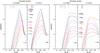 |
Fig. 1 3He profile (in mass fraction) at the main-sequence turnoff for models of various masses as indicated and for two values of the metallicity (Z = 10-4 and Z⊙ in the left and right subpanels respectively). The horizontal arrows indicate the initial 3He content assumed at stellar birth. The vertical lines show, in each case, the maximum depth reached by the convective envelope during the first dredge-up. (Left) Standard models. (Right) Models including rotation-induced mixing, assuming an initial rotation velocity equal to 45% of the critical velocity on the zero age main sequence; for the [2, 4 M⊙; Z⊙ and Z = 10-04] rotating models, the dotted curves correspond to predictions assuming VZAMS/Vcrit ~ 0.90. |
When stars move towards the RGB, their convective envelope deepens until they reach the region indicated by the vertical lines in Fig. 1, and engulfs all or part of the fresh 3He peak. The first dredge-up efficiency (in terms of maximum penetration depth of the convective envelope) decreases with decreasing metallicity as shown in Fig. 2 (at Z = 10-4, no first dredge-up occurs for stars more massive than ~3.0 M⊙). As a consequence, the surface abundance of 3He increases by a factor that depends on the initial stellar mass as well as on the metallicity, as can be seen in Figs. 3 − 57.
During the subsequent evolution on the RGB that proceeds on shorter timescales compared to the main-sequence lifetime, H-burning is concentrated in a very small (both in mass and radius) radiative shell that surrounds the degenerate helium core and is dominated by the CNO-cycle. There is thus no significant further 3He production inside evolved stars. In addition, the temperature in their convective envelope remains always low enough to preserve the freshly dredged-up 3He. Consequently and as far as standard models are concerned, there is no other change in the 3He surface abundance until the stars undergo the second dredge-up on the early-AGB. During this short episode the convective envelope deepens again (see Fig. 2) and reaches 3He-free regions, which induces a slight decrease of the surface abundance of this element (see Figs. 3–5).
Except in the few cases discussed below (see Tables 1 to 4), we stopped our standard computations at that phase. For low-mass stars the standard models published in the literature predict that the 3He stored in the stellar convective envelope survives the TP-AGB phase before it is injected into the ISM by stellar wind and planetary nebula ejection (see references in Sect. 3.1.2). This agrees with our standard [1.5, 2 M⊙; Z⊙], [1.0; Z = 0.004], and [1.0, 1.5 M⊙; Z = 0.002] models that we computed up to the AGB tip and for which surface 3He abundance remains constant during the TP-AGB phase. Note, however, that in stars with initial masses higher than ~3.5−4 M⊙, hot-bottom burning during the TP-AGB phase induces 3He-burning at the base of the convective envelope and thus reduces the abundance of this element in the whole envelope and at the stellar surface (Sackmann & Boothroyd 1992; Weiss et al. 1996; Forestini & Charbonnel 1997; Sackmann & Boothroyd 1999). Because of this process 3He can even be completely destroyed at the AGB tip in the most massive intermediate-mass stars (see the standard [6 M⊙; Z⊙] model in Fig. 4), so that the corresponding net yields are negative. This will be discussed in more detail in Sect. 3.2, where we present the computations up to the TP-AGB tip for complete models including the effects of thermohaline and rotation-induced mixing.
3.1.2. Surface abundances prior to the TP-AGB and comparison with standard models from the litterature
In Fig. 5 we present the standard predictions for the surface abundance of 3He after both first and second dredge-up episodes (solid and dashed lines respectively) as a function of initial stellar mass for the four considered metallicity values. Note that the 3 to 6 M⊙ models at Z = 0.0001 do not undergo the first dredge-up (see Fig. 2). In this case we show the 3He surface abundance at the end of the main sequence and after second dredge-up (solid and dashed).
The assumed initial 3He abundance as well as the total initial D + 3He are also indicated in Fig. 5. This confirms that in the standard case, stars with an initial mass lower than ~ 3.5 − 4 M⊙ that do not undergo hot-bottom burning are expected to strongly enrich the Universe with 3He. The mass dependency described above also clearly shows up.
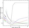 |
Fig. 2 Maximum depth in mass of the convective envelope relative to the total stellar mass reached during first and second dredge-up (solid and dashed lines respectively) as a function of initial stellar mass and for the different metallicities, as indicated by the colours of the curves. |
In this figure we also compare our standard predictions with those by Weiss et al. (1996) and Sackmann & Boothroyd (1999) at solar metallicity on one hand, and those by Sackmann & Boothroyd (1999) for Z = 10-4 on the other hand. An excellent agreement is found with these standard theoretical models.
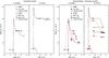 |
Fig. 3 Evolution of the surface abundance of 3He as a function of stellar luminosity for 1.5 M⊙ models with Z = 10-4 and Z⊙ as indicated. Main evolution steps are pointed out with different symbols.(Left) Standard case computed up to the end of the second dredge-up only. (Right) Models including either thermohaline mixing only (black solid lines), or both thermohaline and rotation-induced mixing (red dashed lines; VZAMS/Vcrit = 0.45); at Z⊙ the non-standard models are both computed up to the AGB tip. |
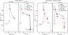 |
Fig. 4 Same as Fig. 3 for 6 M⊙ models (but with different ordinate). (Left) Standard case. The low-metallicity model is computed up to the end of second dredge-up only, while the Z⊙ one is carried out until the AGB tip. (Right) Models including thermohaline mixing only (black solid lines), and including both thermohaline and rotation-induced mixings (red dashed lines; VZAMS/Vcrit = 0.45). These rotating models are computed until the AGB tip. |
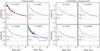 |
Fig. 5 Surface abundance of 3He (in mass fraction) at the end of first and second dredge-up episodes (solid and dashed black lines respectively) as a function of initial stellar mass and for the four metallicities considered (for the 3 to 6 M⊙ standard models at Z = 0.0001 that do not undergo first dredge-up, we show instead the 3He surface abundance at the main-sequence turnoff). Red dotted curves indicate the initial 3He abundance and total D + 3He assumed at stellar birth. (Left) Standard models. Full red triangles correspond to the predictions by Weiss et al. (1996) at the end of 1DUP for Z⊙; blue circles (open and full at the end of 1DUP and 2DUP respectively) are predictions by Sackmann & Boothroyd (1999) for Z⊙ and Z = 10-4. (Right) Models including thermohaline and rotation-induced mixings. |
3.2. Models including rotation-induced mixing and thermohaline instability
In Paper I we discussed at length the impact of both rotation-induced mixing and thermohaline instability on the structure and chemical properties of low- and intermediate-mass stars at various phases of their evolution. Here we only briefly summarize the main points, focusing on 3He.
Note that in low-mass stars, thermohaline mixing induced by the molecular-weight inversion due to the 3He(3He, 2p)4He reaction sets in only at the RGB bump. Up to that phase, predictions for models including only this process (i.e., not including rotation-induced effects) are therefore similar to the standard ones described above (in particular the predictions are the same for 3He surface values caused by first dredge-up), and they start differing only on the upper RGB. In the case of intermediate-mass stars, thermohaline mixing starts playing a role even later, i.e., on the TP-AGB phase. However, rotation-induced mixing has an impact already in the earlier phases for all stellar masses, as described below.
3.2.1. Main-sequence abundance profiles and first dredge-up
As known for a long time (see references in Paper I), rotation-induced mixing modifies the internal structure of main-sequence stars, and smoothes out the abundance gradients with respect to the standard case. Consequently, the 3He production is moderatly affected by the slightly higher temperature in the rotating models compared to the standard case for a given stellar mass and metallicity during central H-burning. But more importantly, the 3He peak is spread out and fresh 3He is expected to reach the stellar surface during the main-sequence lifetime. The resulting profiles at turnoff are shown in Fig. 1 and can be compared to the standard ones (left and right panels respectively). At that evolution point, the total 3He content for a star of given initial stellar mass and metallicity is slightly lower in the rotating case. As can be seen in Fig. 1, the higher the initial rotation velocity, the stronger the effect.
Additionally, the structural and chemical changes caused by rotation on the main sequence favour a slightly deeper penetration of the convective envelope during the subsequent first dredge-up episode (because the mass of the He-core is slightly larger at the end of the main sequence in the rotating case), which leads to the engulfment of larger 3He-free regions that lie below the peak. As a consequence, post dredge-up 3He values are lower when rotation is accounted for than in the standard models, as can be seen in Figs. 3 − 5, and in Tables 1 to 4. The effects are stronger for increasing stellar mass and decreasing metallicity.
3.2.2. Red giant branch
In the advanced evolution phases the total diffusion coefficient associated to rotation is too low to induce abundance changes at the stellar surface (see below, and also Chanamé et al. 2005; Palacios et al. 2006; Cantiello & Langer 2008, 2010; and Paper I) However, for low-mass stars the surface abundances change after the RGB bump with respect to the post dredge-up values, because of thermohaline mixing induced by the molecular weight inversion created by the 3He(3He, 2p)4He reaction in the outer wing of the hydrogen-burning shell. Figure 6 compares the diffusion coefficient associated to the thermohaline instability, Dthc, for a 1.25 M⊙ star at different metallicities, to the total diffusion coefficient associated to rotation, Drot, that characterizes the transport of chemicals caused by meridional circulation and shear turbulence. For each model these quantities are shown at the evolution point on the RGB when the surface abundances start changing because of thermohaline mixing (this refers to the evolution point C1.25 in Fig. 1 of Paper I) . In all cases, Dthc is at least 2 to 3 orders of magnitude higher than Drot (see also Paper I; and Cantiello & Langer 2008, 2010).
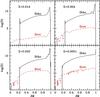 |
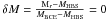
Fig. 6 Thermohaline diffusion coefficient, Dthc, and total rotation diffusion coefficient, Drot, (solid and dashed lines respectively) as a function of reduced stellar mass, δM ( |
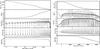 |
Fig. 7 (From top to bottom) Evolution along the TP-AGB of the surface abundance of 3He, of N(Li), of the temperature at the base of convective envelope, of the helium-burning luminosity, and of the total stellar mass. The abscissa is the time since the first thermal pulse. Left and right respectively: 2.5 and 6 M⊙ at Z⊙ models computed with thermohaline and rotation-induced mixings. |
As discussed in detail in Paper I and in Charbonnel & Zahn (2007b), the present prescription for the thermohaline diffusivity accounts for the observed behaviour of 12C/13C, [N/C], and lithium in low-mass stars that are more luminous than the RGB bump. It simultaneously leads to strong 3He depletion in the stellar envelope, as can be seen in Fig. 3 (see also e.g. Charbonnel & Zahn 2007b). However, 3He is not completely destroyed at the RGB tip, and therefore it can drive the thermohaline instability in the latter evolution phases, as discussed below.
3.2.3. Early-AGB and 3He surface abundances after the second dredge-up
In stars with initial masses lower than, or equal to 2 and 1.5 M⊙ for Z = Z⊙ and Z = 0.0001 respectively (with intermediate values for the upper mass limit for the intermediate metallicities), the 3He abundance continues to decrease at the stellar surface between the end of central helium burning and the second dredge-up episode through thermohaline mixing, as can be seen in Fig. 3. On the other hand, in more massive stars rotation induces a decrease of the 3He surface abundance during central helium burning and on the early-AGB (see Fig. 4) before they undergo the second dredge-up (Fig. 2). When integrated over the whole evolution, changing VZAMS/Vcrit from 0.45 to ~ 0.9 leads to a decrease of the 3He surface abundance after the second dredge-up of ~5, 11.5, and 22, 23% in the [2 M⊙; Z⊙], [4 M⊙; Z⊙], and [2 M⊙; Z = 10-04], [4 M⊙; Z = 10-04] models respectively (see Table 4).
The resulting surface 3He values after second dredge-up are shown in Fig. 5 (right panels) for the non-standard models over the whole mass and metallicity range. In summary, compared to the standard case (left panels), one finds that the thermohaline instability dominates in reducing the 3He content of low-mass stars, while the dominating process is rotation for intermediate-mass stars. The impact of both mechanisms increases with decreasing metallicity.
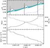 |
Fig. 8 Zoom on the effect of thermohaline mixing between the thermal pulses number 7 and 9 for the 2.5 M⊙ rotating model at Z⊙. (Bottom) Kippenhahn diagram. The hatched zone is the convective envelope; the blue shaded region corresponds to the layers where the thermohaline instability develops; the green and blue dashed lines surround the hydrogen and the helium burning shell respectively (in both cases, the dotted lines show the region of maximum nuclear energy production). (Middle) Evolution of the surface 7Li abundance (full line) and 12C/13C ratio (dashed line). (Bottom) Evolution of the surface 3He abundance (in mass fraction). |
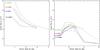 |
Fig. 9 Yields of 3He as a function of stellar mass, at different metallicities. (Left) Predictions for standard models. (Right) Predictions including thermohaline mixing only (solid lines) and including both thermohaline and rotation-induced mixings (dashed lines, for models computed up to the AGB tip or to 3He exhaustion). |
3.2.4. TP-AGB
After the second dredge-up, 3He remains in sufficient quantity to drive thermohaline mixing during the TP-AGB in stars that do not undergo hot-bottom burning (i.e., with initial mass below ~3 M⊙). As discussed in Paper I (see also Cantiello & Langer 2010; Stancliffe 2010), this leads to even greater (although modest) depletion of 3He associated to 7Li production during that phase. This is depicted in Fig. 7 as a function of time since the first thermal pulse for a rotating [2.5 M⊙; Z⊙] model computed with thermohaline mixing up to the AGB tip (left panels). This figure also shows the temperature at the base of the convective envelope, the helium-burning luminosity, and the total stellar mass. When compared to the [1.25 M⊙; Z⊙] model discussed in Fig. 7 of Paper I, a slight difference shows up. In the 2.5 M⊙ and from pulse number four on, the convective envelope deepens immediatly after each pulse inside the thermohaline region, re-inforcing the thermohaline effect modifying the surface abundances, as can be seen in Fig. 8 (which focusses on pulses number 7 to 9). Note, however, that the decrease of 3He at the stellar surface owing to the whole process along the TP-AGB is modest, and that 3He is not completely destroyed when these stars reach the TP-AGB tip (see also Tables 1 to 3). In this framework low-mass stars accordingly remain net 3He producers.
Figure 7 also shows the evolution during TP-AGB of 3He and 7Li abundances at the surface of the non-standard [6.0 M⊙, Z⊙] model. For such a relatively massive star 3He is not abundant enough to drive thermohaline mixing during thermal pulses. However, the temperature at the base of the convective envelope is sufficient to engage hot-bottom burning. As a consequence, the surface abundance of 3He decreases very rapidly, until complete destruction. The simultaneous 7Li enrichment at the stellar surface is caused in this case by the Cameron & Fowler (1971) process.
4. Yields of 3He and conclusions
We can now summarize our study by quantifying in terms of yields the impact of thermohaline instability and rotation-induced mixing on the production and destruction of 3He by low- and intermediate-mass stars at various metallicities. The net yields of 3He are shown in Fig. 9 for all our models and are also given in Tables 1 to 4. There one can find for selected models comparisons between the yields obtained when computing the models until the end of second dredge-up only (case A), or up to the AGB tip (case C). Because the decrease of 3He caused by thermohaline mixing during the TP-AGB is very modest for low-mass stars compared to what happens on the RGB, the difference between the extrapolated yields (A) and the ones obtained from the full computations (C) is below ~12% only.
Our main results may be summarized as follows:
-
Over the whole mass and metallicity range considered, the total3He content is lowered when rotation-induced mixing is accounted for compared to the standard case.
-
For low-mass stars (M < 2−2.2 M⊙) that produce large quantities of this light element through the pp-chains on the main sequence, thermohaline mixing on both the RGB and the TP-AGB is dominant in reducing the final 3He yield. These stars remain net producers of 3He however, although their contribution to the Galactic evolution of this light element is strongly reduced compared to the standard framework.
-
For intermediate-mass stars thermohaline mixing does not operate on the shorter RGB (these stars ignite central He-burning before reaching the RGB bump).
-
For those with masses between 2−2.2 and 3−4 M⊙, thermohaline mixing leads however to modest 3He depletion during the TP-AGB phase, associated with lithium production.
-
In more massive intermediate-mass stars, 3He is strongly reduced through the action of rotation that lowers the upper mass limit for stars that are net 3He producers, and is additionally destroyed through hot-bottom burning while they climb the TP-AGB. In these objects Li is produced through the classical Cameron-Fowler mechanism.
The impact on Galactic evolution predictions of these new 3He yields will be presented in a forthcoming paper.
Classical (or standard) stellar models consider convection as the only mixing mechanism inside stars, and neglect all possible transport processes in stellar radiative regions.
The average abundance in Galactic HII regions is 3He/H = (1.9 ± 0.6) × 10-5 (Bania et al. 2002). The protosolar and SBBN-WMAP values are 3He/H = (1.5 ± 0.2) × 10-5 (Geiss & Gloeckler 1998) and 3He/H = (1.04 ± 0.04) × 10-5 (Coc et al. 2004).
Attention to the local depression of μ occurring in RGB stars was drawn by Eggleton et al. (2006), although the peculiarity of this nuclear reaction that converts two particles into three was already pointed out by Ulrich (1971) in a different stellar context.
We define low-mass stars as those that climb the red giant branch with a degenerate helium core; their initial mass is typically lower than 2 − 2.2 M⊙ depending on metallicity. Intermediate-mass stars are those that ignite central helium-burning in a non-degenerate core at relatively low luminosity on the RGB, and finish their lives as C-O white dwarfs.
We do not compute models for more massive stars (i.e., with initial mass higher than ~6 M⊙) that are anyway considered as net 3He destroyers within the standard framework since a large amount of their material is processed at temperatures high enough to burn any present 3He to 4He or beyond (Dearborn et al. 1986).
The ratio measuring the enrichment in 4He reported to the enrichment in heavy elements in the Galaxy until the birth of the Sun is taken equal to ΔY/ΔZ = 1.29 (see Lagarde et al., Paper III, in prep.). We assume [α/Fe] = 0 at all metallicities, which has a negligible impact on the final yields of 3He. Indeed, for the [1.5 M⊙; Z = 0.0001] models the 3He yields are only ~4.6−4.7% (standard and thermohaline cases respectively) higher when [α/Fe] is increased to 0.3.
The evolution of the 3He abundance at the surface of 6 M⊙ standard models depicted in Fig. 4 for the two extreme Z values shows a couple of peculiarities compared to the case of low-mass stars. For such a relatively massive star, the base of the convective envelope withdraws very quickly on the pre-main sequence, precluding any increase of the surface 3He during that phase. However, because of mass loss, the layers enriched in 3He by pristine D-burning appear at the surface later on. In addition, no first dredge-up occurs in the lowest Z 6 M⊙ model (see also Fig. 5).
Acknowledgments
We thank J.-P. Zahn, C. Chiappini, D. Romano, M. Tosi, T. Bania, R. T. Rood and D. Balser for fruitful discussions on the 3He problem over the years. We acknowledge financial support from the Swiss National Science Foundation (FNS), from ESF-Euro Genesis, and the french Programme National de Physique Stellaire (PNPS) of CNRS/INSU.
References
- Angulo, C., Arnould, M., Rayet, M., et al. 1999, Nucl. Phys. A, 656, 3 [NASA ADS] [CrossRef] [Google Scholar]
- Balser, D. S., Bania, T. M., Brockway, C. J., Rood, R. T., & Wilson, T. L. 1994, ApJ, 430, 667 [NASA ADS] [CrossRef] [Google Scholar]
- Balser, D. S., Bania, T. M., Rood, R. T., & Wilson, T. L. 1997, ApJ, 483, 320 [NASA ADS] [CrossRef] [Google Scholar]
- Balser, D. S., Bania, T. M., Rood, R. T., & Wilson, T. L. 1999, ApJ, 510, 759 [NASA ADS] [CrossRef] [Google Scholar]
- Balser, D. S., Goss, W. M., Bania, T. M., & Rood, R. T. 2006, ApJ, 640, 360 [NASA ADS] [CrossRef] [Google Scholar]
- Bania, T. M., Balser, D. S., Rood, R. T., Wilson, T. L., & Wilson, T. J. 1997, ApJS, 113, 353 [NASA ADS] [CrossRef] [Google Scholar]
- Bania, T. M., Rood, R. T., & Balser, D. S. 2002, Nature, 415, 54 [NASA ADS] [CrossRef] [PubMed] [Google Scholar]
- Bania, T. M., Rood, R. T., & Balser, D. S. 2010, in IAU Symp. 268, ed. C. Charbonnel, M. Tosi, F. Primas & C. Chiappini, 81 [Google Scholar]
- Cameron, A. G. W., & Fowler, W. A. 1971, ApJ, 164, 111 [Google Scholar]
- Cantiello, M., & Langer, N. 2008, in IAU Symp. 252, ed. L. Deng & K. L. Chan, 103 [Google Scholar]
- Cantiello, M., & Langer, N. 2010, A&A, 521, A9 [NASA ADS] [CrossRef] [EDP Sciences] [Google Scholar]
- Chanamé, J., Pinsonneault, M., & Terndrup, D. M. 2005, ApJ, 631, 540 [NASA ADS] [CrossRef] [Google Scholar]
- Charbonnel, C. 1994, A&A, 282, 811 [NASA ADS] [Google Scholar]
- Charbonnel, C. 1995, ApJ, 453, L41 [NASA ADS] [CrossRef] [Google Scholar]
- Charbonnel, C., & Do Nascimento, Jr., J. D. 1998, A&A, 336, 915 [NASA ADS] [Google Scholar]
- Charbonnel, C., & Lagarde, N. 2010a, A&A, 522, A10 [NASA ADS] [CrossRef] [EDP Sciences] [MathSciNet] [PubMed] [Google Scholar]
- Charbonnel, C., & Lagarde, N. 2010b, in IAU Symp. 268, ed. C. Charbonnel, M. Tosi, F. Primas & C. Chiappini [Google Scholar]
- Charbonnel, C., & Zahn, J. 2007a, A&A, 476, L29 [NASA ADS] [CrossRef] [EDP Sciences] [Google Scholar]
- Charbonnel, C., & Zahn, J.-P. 2007b, A&A, 467, L15 [NASA ADS] [CrossRef] [EDP Sciences] [Google Scholar]
- Charbonnel, C., Brown, J. A., & Wallerstein, G. 1998, A&A, 332, 204 [NASA ADS] [Google Scholar]
- Chiappini, C., Renda, A., & Matteucci, F. 2002, A&A, 395, 789 [NASA ADS] [CrossRef] [EDP Sciences] [Google Scholar]
- Coc, A., Vangioni-Flam, E., Descouvemont, P., Adahchour, A., & Angulo, C. 2004, ApJ, 600, 544 [NASA ADS] [CrossRef] [Google Scholar]
- Cyburt, R. H., Fields, B. D., & Olive, K. A. 2008, J. Cosmology Astropart. Phys., 11, 12 [Google Scholar]
- Dearborn, D. S. P., Schramm, D. N., & Steigman, G. 1986, ApJ, 302, 35 [NASA ADS] [CrossRef] [Google Scholar]
- Dearborn, D. S. P., Steigman, G., & Tosi, M. 1996, ApJ, 465, 887 [NASA ADS] [CrossRef] [Google Scholar]
- Decressin, T., Mathis, S., Palacios, A., et al. 2009, A&A, 495, 271 [NASA ADS] [CrossRef] [EDP Sciences] [Google Scholar]
- Denissenkov, P. A. 2010, ApJ, 723, 563 [NASA ADS] [CrossRef] [Google Scholar]
- Denissenkov, P. A., & Merryfield, W. J. 2011, ApJ, 727, L8 [NASA ADS] [CrossRef] [Google Scholar]
- Dobbie, P. D., Napiwotzki, R., Burleigh, M. R., et al. 2006, MNRAS, 369, 383 [NASA ADS] [CrossRef] [Google Scholar]
- Dunkley, J., Komatsu, E., Nolta, M. R., et al. 2009, ApJS, 180, 306 [NASA ADS] [CrossRef] [Google Scholar]
- Eggleton, P. P., Dearborn, D. S. P., & Lattanzio, J. C. 2006, Science, 314, 1580 [NASA ADS] [CrossRef] [PubMed] [Google Scholar]
- Eggleton, P. P., Dearborn, D. S. P., & Lattanzio, J. C. 2008, ApJ, 677, 581 [NASA ADS] [CrossRef] [Google Scholar]
- Forestini, M., & Charbonnel, C. 1997, A&AS, 123, 241 [NASA ADS] [CrossRef] [EDP Sciences] [Google Scholar]
- Galli, D., Palla, F., Ferrini, F., & Penco, U. 1995, ApJ, 443, 536 [NASA ADS] [CrossRef] [Google Scholar]
- Galli, D., Stanghellini, L., Tosi, M., & Palla, F. 1997, ApJ, 477, 218 [NASA ADS] [CrossRef] [Google Scholar]
- Geisler, D., Smith, V. V., Wallerstein, G., Gonzalez, G., & Charbonnel, C. 2005, AJ, 129, 1428 [NASA ADS] [CrossRef] [Google Scholar]
- Geiss, J., & Gloeckler, G. 1998, Space Sci. Rev., 84, 239 [NASA ADS] [CrossRef] [Google Scholar]
- Geiss, J., & Gloeckler, G. 2010, in IAU Symp. 268, ed. C. Charbonnel, M. Tosi, F. Primas & C. Chiappini, 71 [Google Scholar]
- Gilroy, K. K. 1989, ApJ, 347, 835 [NASA ADS] [CrossRef] [Google Scholar]
- Gilroy, K. K., & Brown, J. A. 1991, ApJ, 371, 578 [NASA ADS] [CrossRef] [Google Scholar]
- Gratton, R. G., Sneden, C., Carretta, E., & Bragaglia, A. 2000, A&A, 354, 169 [NASA ADS] [Google Scholar]
- Hogan, C. J. 1995, ApJ, 441, L17 [NASA ADS] [CrossRef] [Google Scholar]
- Iben, Jr., I. 1967, ApJ, 147, 624 [NASA ADS] [CrossRef] [Google Scholar]
- Kippenhahn, R., Ruschenplatt, G., & Thomas, H.-C. 1980, A&A, 91, 175 [NASA ADS] [Google Scholar]
- Krishnamurti, R. 2003, J. Fluid Mech., 483, 287 [NASA ADS] [CrossRef] [Google Scholar]
- Maeder, A., & Zahn, J.-P. 1998, A&A, 334, 1000 [NASA ADS] [Google Scholar]
- Olive, K. A., Rood, R. T., Schramm, D. N., Truran, J., & Vangioni-Flam, E. 1995, ApJ, 444, 680 [NASA ADS] [CrossRef] [Google Scholar]
- Palacios, A., Charbonnel, C., Talon, S., & Siess, L. 2006, A&A, 453, 261 [NASA ADS] [CrossRef] [EDP Sciences] [Google Scholar]
- Palla, F., Bachiller, R., Stanghellini, L., Tosi, M., & Galli, D. 2000, A&A, 355, 69 [NASA ADS] [Google Scholar]
- Pilachowski, C., Sneden, C., Freeland, E., & Casperson, J. 2003, AJ, 125, 794 [NASA ADS] [CrossRef] [Google Scholar]
- Recio-Blanco, A., & de Laverny, P. 2007, A&A, 461, L13 [NASA ADS] [CrossRef] [EDP Sciences] [Google Scholar]
- Reimers, D. 1975, Mem. Soc. Roy. Sci. Liege, 8, 369 [Google Scholar]
- Rood, R. T., Steigman, G., & Tinsley, B. M. 1976, ApJ, 207, L57 [NASA ADS] [CrossRef] [Google Scholar]
- Rood, R. T., Wilson, T. L., & Steigman, G. 1979, ApJ, 227, L97 [NASA ADS] [CrossRef] [Google Scholar]
- Romano, D., Tosi, M., Matteucci, F., & Chiappini, C. 2003, MNRAS, 346, 295 [NASA ADS] [CrossRef] [Google Scholar]
- Rood, R. T., Bania, T. M., & Wilson, T. L. 1984, ApJ, 280, 629 [NASA ADS] [CrossRef] [Google Scholar]
- Rosenblum, E., Garaud, P., Traxler, A., & Stellmach, S. 2011, ApJ, 731, 66 [NASA ADS] [CrossRef] [Google Scholar]
- Sackmann, I., & Boothroyd, A. I. 1992, ApJ, 392, L71 [NASA ADS] [CrossRef] [Google Scholar]
- Sackmann, I., & Boothroyd, A. I. 1999, ApJ, 510, 217 [NASA ADS] [CrossRef] [Google Scholar]
- Shetrone, M. D. 2003, ApJ, 585, L45 [NASA ADS] [CrossRef] [Google Scholar]
- Smith, V. V., Hinkle, K. H., Cunha, K., et al. 2002, AJ, 124, 3241 [NASA ADS] [CrossRef] [Google Scholar]
- Spergel, D. N., Verde, L., Peiris, H. V., et al. 2003, ApJS, 148, 175 [NASA ADS] [CrossRef] [Google Scholar]
- Spite, M., Cayrel, R., Hill, V., et al. 2006, A&A, 455, 291 [NASA ADS] [CrossRef] [EDP Sciences] [Google Scholar]
- Stancliffe, R. J. 2010, MNRAS, 174 [Google Scholar]
- Stancliffe, R. J., Church, R. P., Angelou, G. C., & Lattanzio, J. C. 2009, MNRAS, 396, 2313 [Google Scholar]
- Tautvaišiene, G., Edvardsson, B., Tuominen, I., & Ilyin, I. 2000, A&A, 360, 499 [NASA ADS] [Google Scholar]
- Tautvaišienė, G., Edvardsson, B., Puzeras, E., & Ilyin, I. 2005, A&A, 431, 933 [NASA ADS] [CrossRef] [EDP Sciences] [Google Scholar]
- Tosi, M. 1996, in From Stars to Galaxies: the Impact of Stellar Physics on Galaxy Evolution, ed. C. Leitherer, U. Fritze-von-Alvensleben & J. Huchra, APS Conf. Ser., 98, 299 [Google Scholar]
- Tosi, M. 1998, Space Sci. Rev., 84, 207 [NASA ADS] [CrossRef] [Google Scholar]
- Tosi, M. 2000, in The Light Elements and their Evolution, ed. L. da Silva, R. de Medeiros & M. Spite, IAU Symp., 198, 525 [Google Scholar]
- Traxler, A., Garaud, P., & Stellmach, S. 2011, ApJ, 728, L29 [NASA ADS] [CrossRef] [Google Scholar]
- Ulrich, R. K. 1971, ApJ, 168, 57 [NASA ADS] [CrossRef] [Google Scholar]
- Ulrich, R. K. 1972, ApJ, 172, 165 [NASA ADS] [CrossRef] [Google Scholar]
- Vassiliadis, E., & Wood, P. R. 1993, ApJ, 413, 641 [NASA ADS] [CrossRef] [Google Scholar]
- Wachlin, F. C., Miller Bertolami, M. M., & Althaus, L. G. 2011, A&A, 533, A139 [NASA ADS] [CrossRef] [EDP Sciences] [Google Scholar]
- Weiss, A., Wagenhuber, J., & Denissenkov, P. A. 1996, A&A, 313, 581 [NASA ADS] [Google Scholar]
- Wilson, T. L., & Rood, R. 1994, ARA&A, 32, 191 [NASA ADS] [CrossRef] [Google Scholar]
- Zahn, J.-P. 1992, A&A, 265, 115 [NASA ADS] [Google Scholar]
All Tables
All Figures
|
Fig. 1 3He profile (in mass fraction) at the main-sequence turnoff for models of various masses as indicated and for two values of the metallicity (Z = 10-4 and Z⊙ in the left and right subpanels respectively). The horizontal arrows indicate the initial 3He content assumed at stellar birth. The vertical lines show, in each case, the maximum depth reached by the convective envelope during the first dredge-up. (Left) Standard models. (Right) Models including rotation-induced mixing, assuming an initial rotation velocity equal to 45% of the critical velocity on the zero age main sequence; for the [2, 4 M⊙; Z⊙ and Z = 10-04] rotating models, the dotted curves correspond to predictions assuming VZAMS/Vcrit ~ 0.90. |
| In the text | |
|
Fig. 2 Maximum depth in mass of the convective envelope relative to the total stellar mass reached during first and second dredge-up (solid and dashed lines respectively) as a function of initial stellar mass and for the different metallicities, as indicated by the colours of the curves. |
| In the text | |
|
Fig. 3 Evolution of the surface abundance of 3He as a function of stellar luminosity for 1.5 M⊙ models with Z = 10-4 and Z⊙ as indicated. Main evolution steps are pointed out with different symbols.(Left) Standard case computed up to the end of the second dredge-up only. (Right) Models including either thermohaline mixing only (black solid lines), or both thermohaline and rotation-induced mixing (red dashed lines; VZAMS/Vcrit = 0.45); at Z⊙ the non-standard models are both computed up to the AGB tip. |
| In the text | |
|
Fig. 4 Same as Fig. 3 for 6 M⊙ models (but with different ordinate). (Left) Standard case. The low-metallicity model is computed up to the end of second dredge-up only, while the Z⊙ one is carried out until the AGB tip. (Right) Models including thermohaline mixing only (black solid lines), and including both thermohaline and rotation-induced mixings (red dashed lines; VZAMS/Vcrit = 0.45). These rotating models are computed until the AGB tip. |
| In the text | |
|
Fig. 5 Surface abundance of 3He (in mass fraction) at the end of first and second dredge-up episodes (solid and dashed black lines respectively) as a function of initial stellar mass and for the four metallicities considered (for the 3 to 6 M⊙ standard models at Z = 0.0001 that do not undergo first dredge-up, we show instead the 3He surface abundance at the main-sequence turnoff). Red dotted curves indicate the initial 3He abundance and total D + 3He assumed at stellar birth. (Left) Standard models. Full red triangles correspond to the predictions by Weiss et al. (1996) at the end of 1DUP for Z⊙; blue circles (open and full at the end of 1DUP and 2DUP respectively) are predictions by Sackmann & Boothroyd (1999) for Z⊙ and Z = 10-4. (Right) Models including thermohaline and rotation-induced mixings. |
| In the text | |
|
Fig. 6 Thermohaline diffusion coefficient, Dthc, and total rotation diffusion coefficient, Drot, (solid and dashed lines respectively) as a function of reduced stellar mass, δM ( |
| In the text | |
|
Fig. 7 (From top to bottom) Evolution along the TP-AGB of the surface abundance of 3He, of N(Li), of the temperature at the base of convective envelope, of the helium-burning luminosity, and of the total stellar mass. The abscissa is the time since the first thermal pulse. Left and right respectively: 2.5 and 6 M⊙ at Z⊙ models computed with thermohaline and rotation-induced mixings. |
| In the text | |
|
Fig. 8 Zoom on the effect of thermohaline mixing between the thermal pulses number 7 and 9 for the 2.5 M⊙ rotating model at Z⊙. (Bottom) Kippenhahn diagram. The hatched zone is the convective envelope; the blue shaded region corresponds to the layers where the thermohaline instability develops; the green and blue dashed lines surround the hydrogen and the helium burning shell respectively (in both cases, the dotted lines show the region of maximum nuclear energy production). (Middle) Evolution of the surface 7Li abundance (full line) and 12C/13C ratio (dashed line). (Bottom) Evolution of the surface 3He abundance (in mass fraction). |
| In the text | |
|
Fig. 9 Yields of 3He as a function of stellar mass, at different metallicities. (Left) Predictions for standard models. (Right) Predictions including thermohaline mixing only (solid lines) and including both thermohaline and rotation-induced mixings (dashed lines, for models computed up to the AGB tip or to 3He exhaustion). |
| In the text | |
Current usage metrics show cumulative count of Article Views (full-text article views including HTML views, PDF and ePub downloads, according to the available data) and Abstracts Views on Vision4Press platform.
Data correspond to usage on the plateform after 2015. The current usage metrics is available 48-96 hours after online publication and is updated daily on week days.
Initial download of the metrics may take a while.