| Issue |
A&A
Volume 536, December 2011
|
|
|---|---|---|
| Article Number | A58 | |
| Number of page(s) | 24 | |
| Section | Stellar atmospheres | |
| DOI | https://doi.org/10.1051/0004-6361/201117101 | |
| Published online | 07 December 2011 | |
Nitrogen line spectroscopy of O-stars
I. Nitrogen III emission line formation revisited⋆
1
Universitätssternwarte München, Scheinerstr. 1, 81679 München, Germany
e-mail: This email address is being protected from spambots. You need JavaScript enabled to view it.
2
Centro de Astrobiología, (CSIC-INTA), Ctra. Torrejón a Ajalvir km 4, 28850 Torrejón de Ardoz, Spain
Received: 18 April 2011
Accepted: 14 September 2011
Abstract
Context. Evolutionary models of massive stars predict a surface enrichment of nitrogen, due to rotational mixing. Recent studies within the VLT-FLAMES survey of massive stars have challenged (part of) these predictions. Such systematic determinations of nitrogen abundances, however, have been mostly performed only for cooler (B-type) objects. For the most massive and hottest stars, corresponding results are scarce.
Aims. This is the first paper in a series dealing with optical nitrogen spectroscopy of O-type stars, aiming at the analysis of nitrogen abundances for stellar samples of significant size, to place further constraints on the early evolution of massive stars. Here we concentrate on the formation of the optical N iii lines at λλ4634−4640−4642 that are fundamental for the definition of the different morphological “f”-classes.
Methods. We implement a new nitrogen model atom into the NLTE atmosphere/spectrum synthesis code fastwind, and compare the resulting optical Niii spectra with other predictions, mostly from the seminal work by Mihalas & Hummer (1973, ApJ, 179, 827, “MH”), and from the alternative code cmfgen.
Results. Using similar model atmospheres as MH (not blanketed and wind-free), we are able to reproduce their results, in particular the optical triplet emission lines. According to MH, these should be strongly related to dielectronic recombination and the drain by certain two-electron transitions. However, using realistic, fully line-blanketed atmospheres at solar abundances, the key role of the dielectronic recombinations controlling these emission features is superseded – for O-star conditions – by the strength of the stellar wind and metallicity. Thus, in the case of wind-free (weak wind) models, the resulting lower ionizing EUV-fluxes severely suppress the emission. As the mass loss rate is increased, pumping through the N iii resonance line(s) in the presence of a near-photospheric velocity field (i.e., the Swings-mechanism) results in a net optical triplet line emission. A comparison with results from cmfgen is mostly satisfactory, except for the range 30 000 K ≤ Teff ≤ 35 000 K, where cmfgen triggers the triplet emission at lower Teff than fastwind. This effect could be traced down to line overlap effects between the N iii and O iii resonance lines that cannot be simulated by fastwind so far, due to the lack of a detailed O iii model atom.
Conclusions. Since the efficiency of dielectronic recombination and “two electron drain” strongly depends on the degree of line-blanketing/-blocking, we predict the emission to become stronger in a metal-poor environment, though lower wind-strengths and nitrogen abundances might counteract this effect. Weak winded stars (if existent in the decisive parameter range) should display less triplet emission than their counterparts with “normal” winds.
Key words: stars: winds, outflows / stars: early-type / stars: atmospheres / line: formation
Appendices A–C are available in electronic form at http://www.aanda.org
© ESO, 2011
1. Introduction
One of the key aspects of massive star evolution is rotational mixing and its impact. Evolutionary models including rotation (e.g., Heger & Langer 2000; Meynet & Maeder 2000; Brott et al. 2011a) predict a surface enrichment of nitrogen with an associated carbon depletion during the main sequence evolution1. The faster a star rotates, the more mixing will occur, and the larger the nitrogen surface abundance that should be observed.
Several studies (Hunter et al. 2008, 2009b; Brott et al. 2011b) have challenged the predicted effects of rotational mixing on the basis of observations performed within the VLT-FLAMES survey of massive stars (Evans et al. 2006). These studies provide the first statistically significant abundance measurements of Galactic, LMC, and SMC B-type stars, covering a broad range of rotational velocities.
For the Galactic case, the mean B-star nitrogen abundance as derived by Hunter et al. (2009a) is in quite good agreement with the corresponding baseline abundance. For the Magellanic Clouds stars, however, the derived nitrogen abundances show clearly the presence of an enrichment, where this enrichment is more extreme in the SMC than in the LMC2. Theoretical considerations have major difficulties in explaining several aspects of the accumulated results: within the population of (LMC) core-hydrogen burning objects, both unenriched fast rotators and highly enriched slow rotators have been found, in contradiction to standard theory, as well as slowly rotating, highly enriched B-supergiants (see below). Taken together, these results imply that standard rotational mixing might be not as dominant as usually quoted, and/or that other enrichment processes might be present as well (Brott et al. 2011b).
Interestingly, there exist only few rapidly rotating B-supergiants, since there is a steep drop of rotation rates below Teff ≈ 20 kK (e.g., Howarth et al. 1997). Recently, Vink et al. (2010) tried to explain this finding based on two alternative scenarios. In the first scenario, the low rotation rates of B-supergiants are suggested to be caused by braking due to an increased mass loss for Teff < 25 kK, related to the so-called bi-stability jump (Pauldrach & Puls 1990; Vink et al. 2000). Since the reality of such an increased mass loss is still debated (Markova & Puls 2008; Puls et al. 2010), Vink et al. (2010) discuss an alternative scenario where the slowly rotating B-supergiants might form an entirely separate, non core hydrogen-burning population. E.g., they might be products of binary evolution (though this is not generally expected to lead to slowly rotating stars), or they might be post-RSG or blue-loop stars.
Support of this second scenario is the finding that the majority of the cooler (LMC) objects is strongly nitrogen-enriched (see above), and Vink et al. argue that “although rotating models can in principle account for large N abundances, the fact that such a large number of the cooler objects is found to be N enriched suggests an evolved nature for these stars”. A careful nitrogen analysis of their (early) progenitors, the O-type stars, will certainly help to further constrain these ideas and present massive star evolution in general. Note that one of the scientific drivers of the current VLT-FLAMES Tarantula survey (Evans et al. 2011) is just such an analysis of an unprecedented sample of “normal” O-stars and emission-line stars.
Until to date, however, nitrogen abundances have been systematically derived only for the cooler subset of the previous VLT-FLAMES survey, by means of analyzing N ii alone, whereas corresponding results are missing for the most massive and hottest stars. More generally, when inspecting the available literature for massive stars, one realizes that metallic abundances, in particular of the key element nitrogen, have been derived only for a small number of O-type stars (e.g., Bouret et al. 2003; Hillier et al. 2003; Walborn et al. 2004; Heap et al. 2006). The simple reason is that they are difficult to determine, since the formation of N iii/N iv lines (and lines from similar ions of C and O) is problematic due to the impact of various processes that are absent or negligible at cooler spectral types.
One might argue that the determination of nitrogen and other metallic abundances of hotter stars could or even should be performed via UV wind-lines, since these are clearly visible as long as the wind-strength is not too low, and the line-formation is less complex and less dependent on accurate atomic models than for photospheric lines connecting intermediate or even high-lying levels. Note, however, that the results of such analyses strongly depend on the assumptions regarding and the treatment of wind X-ray emission and wind clumping (Puls et al. 2008, and references therein). A careful photospheric analysis, on the other hand, remains rather unaffected by such problems as long as X-ray emission and clumping do not start (very) close to the photosphere, and we will follow the latter approach, concentrating on optical lines.
This paper is the first in a series of upcoming publications dealing with nitrogen spectroscopy of O-type stars. The major objective of this project is the analysis of optical spectra from stellar samples of significant size in different environments, to derive the corresponding nitrogen abundances which are key to our understanding of the early evolution of massive stars. In the present study, we will concentrate on the formation of the optical N iii emission lines at λλ4634 − 4640 − 4642, which are fundamental for the definition of the different morphological “f”-classes. During our implementation of nitrogen into the NLTE-atmosphere/line formation code fastwind (Puls et al. 2005) it turned out that the canonical explanation in terms of dielectronic recombination (Mihalas & Hummer 1973) no longer or only partly applies when modern atmosphere codes including line-blocking/blanketing and winds are used to synthesize the N iii spectrum. Since the f-features are observed in the majority of O-stars and strongly dependent on the nitrogen abundance, a thorough re-investigation of their formation process is required, in order to avoid wrong conclusions.
This paper is organized as follows: at first (Sect. 2) we recapitulate previous explanations for the N iii triplet emission, in particular the standard picture as provided by Mihalas & Hummer (1973). In Sect. 3 we discuss the dielectronic recombination process and its implementation into fastwind. Section 4 presents our new N iii model ion, and in Sect. 5 we investigate the dependence of the triplet emission on various processes. We compare our results with corresponding ones from the alternative code cmfgen (Hillier & Miller 1998) in Sect. 6, and discuss the impact of coupling with O iii via corresponding resonance lines in Sect. 7. The dependence of the emission strength on specific parameters is discussed in Sects. 8, and 9 provides our summary and conclusions.
In the next paper of this series (“Paper II”), we will present our complete nitrogen model atom, and perform a nitrogen abundance analysis for the LMC O-stars from the previous VLT-FLAMES survey of massive stars.
2. N iii emission lines from O-stars – status quo
The presence of emission in the N iii triplet at λλ4634–4640–4642 Å, in combination with the behaviour of He ii λ4686, is used for classification purposes (“f”-features, see Walborn 1971; Sota et al. 2011), and to discriminate O-stars with such line emission from pure absorption-line objects. As stressed by Bruccato & Mihalas (1971, hereafter BM71), these emission lines originate in the stellar photosphere and not in an “exterior shell” (see also Heap et al. 2006, for more recent work). In this case, the most plausible explanation is by invoking NLTE effects. In NLTE, line emission occurs when the corresponding source function at formation depths is larger than the continuum intensity at transition frequency ν0. Such a large source function becomes possible if the upper level of the transition is (considerably) overpopulated with respect to the lower one, i.e., if bu > bl (with bu and bl the NLTE departure coefficients of the upper and lower level, respectively). Note that both coefficients can lie below unity.
For the N iii triplet produced by the 3p–3d transitions (see Fig. 1), such a mechanism should result in a (relative) overpopulation of the upper level, 3d. In the early work about Of stars, the fluorescence mechanism developed by Bowen (1935) has been suggested to trigger such an overpopulation. Many authors (Swings & Struve 1940; Swings 1948; Oke 1954) argued against the relevance of the Bowen mechanism in Of stars, because of the lack of O iii emission lines at λλ3340, 3444, 3759 Å which are connected to the involved levels.
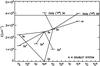 |
Fig. 1 Grotrian diagram displaying the transitions involved in the N iii emission lines problem. The horizontal line marks the N iii ionization threshold. The N iiiλλ4634 − 4640 − 4642 triplet is formed by the transitions 3d → 3p, while the absorption lines at λλ4097-4103 are due to the transitions 3p → 3s. An effective drain of 3p is provided by the “two electron transitions” 3p → 2p |

An alternative suggestion is due to Swings (1948) and relies on an intense continuum that may directly pump the resonance transition 2p → 3d (thus producing the required overpopulation, b3d > b3p) as well as 2p → 3s, while the transition 2p–3p is radiatively forbidden. The implied overpopulation of level 3s due to pumping may then explain why the transitions 3s–3p at λλ4097-4103 are always in absorption (b3s > b3p).
Without such pumping of the 3s level, an auxiliary draining mechanism for the 3p level is needed, since otherwise an overpopulation, b3p > b3s, might occur due to cascade processes, implying the presence of emission at λλ4097-4103, which is not observed. Indeed, the anomalous “two electron transitions” 2p2 (2S, 2P, 2D) – 3p with transition probabilities comparable to the 3p → 3s one electron transition have been identified by Nikitin & Yakubovskii (1963) as potentially important draining processes. Calculations by BM71 show that the presence of these draining processes is sufficient both to ensure the overpopulation of 3d (relative to 3p) and to prevent the overpopulation of 3p relative to 3s. Thus, these “two electron transitions” play a key role.
BM71 also noted a problem for the Swings mechanism when applied to realistic conditions. The 2p → 3s and 2p → 3d resonance lines are expected to be much more opaque than 3p → 3s and 3d → 3p, and should be consequently in detailed balance in the line forming region. That would mean no pumping and no overpopulation of 3d relative to 3p (but see Sect. 5.3). The problem became (preliminary) solved when BM71 suggested a third potential mechanism. They realized the existence of a large number of autoionizing levels that either connect directly to the 3d state or to levels that can cascade downwards to 3d. Hence, the latter state may become strongly overpopulated by dielectronic recombination (“DR”, see Sect. 3).
The most influential analysis of the N iii emission lines problem until now has been carried out by Mihalas & Hummer (1973, “MH”), building on the work by BM71. They used static, plane-parallel models trying to explain the effect for O((f)) and O(f) stars. As a final result, they were able to reproduce the N iii triplet emission at the observed temperatures and gravities in parallel with absorption at λλ4097 − 4103, by overpopulating level 3d primarily via dielectronic recombination. The subsequent 3d → 3p cascade produces the emission. The strong drain 3p → 2p2 via “two electron transitions” enhances the overpopulation of 3d relative to 3p by depopulating 3p and prevents emission in the 3p → 3s lines. Until to-date, dielectronic recombination is the canonical explanation for the formation of the f-features.
3. Dielectronic recombination
If two electrons are excited within a complex atom/ion with several electrons, they can give rise to states with energies both below and above the ionization potential. States above the ionization limit, under certain selection rules, may preferentially autoionize to the ground state of the ion plus a free electron.
Thus the ionization from an initial bound state A(i) to an ionized final state A+(f) can occur either directly, or by a (different) transition from the initial bound state A(i) to an intermediate doubly excited state  above the ionization potential that finally autoionizes to A+(f). In this respect, Photo-Excitation of the Core (PEC) resonances (Yan & Seaton 1987) are particularly strong, because they correspond to a single electron transition in which the outer electron is a spectator and does not change.
The inverse process is also possible, if an ion collides with an electron of sufficient energy, leading to a doubly excited state. Generally, the compound state will immediately autoionize again (large autoionization probabilities, Aa ~ 1013 − 1014 s-1). In some cases, however, a stabilizing transition occurs, in which one of the excited electrons, usually the one in the lower state, radiatively decays to the lowest available quantum state. This process is the dielectronic recombination, and can be summarized as the capture of an electron by the target leading to an intermediate doubly excited state that stabilises by emitting a photon rather than an electron.
3.1. The N iii emission triplet at λλ4634–4640–4642
As pointed out by Mihalas (1971), there are two important autoionizing series in the N iii ion, of the form 2s2p(1P°)nl and 2s2p(3P°)nl, along with few bound double excitation states with similar configuration. Since states of the form 2s2pnl are directly coupled to 2s2nl states, they are of great importance. In the following, we consider only the states from the singlet series, because the transitions from the triplet series to 2s2nl states are not electric dipole allowed transitions in LS coupling.
The singlet series comprises only two bound configurations, 2s2p3s and 2s2p3p, whilst the 2s2p3d configuration lies only 1.6 eV above the ionization potential and is of major importance, since the low position in the continuum produces strong dielectronic recombination,  (1)Note that the core electron transition (see above), 2s2(1S) → 2s2p(1P°), is equivalent to the resonance transition in N iv. Thus, any 2s2(1S)nl → 2s2p(1P°)nl transition gives rise to strong, broad resonances (see Fig. 2), unless the 2s2p(1P°)nl state is truly bound.
The autoionizing states (Eq. (1)) can stabilize via two alternative routes, either  (2)that end in the doubly excited bound configuration mentioned above, or the one that might overpopulate the upper level of the transition 3d → 3p,
  (3)thus playing a (potential) key role in the N iii triplet emission. The latter route is displayed in the upper part of Fig. 1.
3.2. Implementation into fastwind
Dielectronic recombination and its inverse process have been implemented into fastwind in two different ways, to allow us to use different data sets. Specifically, we implemented
-
(i)
an implicit method where the contribution of the dielectronicrecombination is already included in the photoionizationcross-sections. This method needs to be used for data that has beencalculated, e.g., within the OPACITY project (Cunto &Mendoza 1992); and
-
(ii)
an explicit method using resonance-free photoionization cross-sections in combination with explicitly included stabilizing transitions from autoionizing levels. This method will be used when we have information regarding transition frequencies and strengths of the stabilizing transitions.
Later on we discuss the advantages and disadvantages of both methods, whereas in Appendix A.1 we provide some details on the explicit method, and in Appendix A.2 we show that the implicit and explicit method are consistent as long as the autoionizing states are in LTE, as often the case (or frequently assumed).
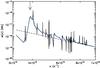 |
Fig. 2 Comparison of the “raw” cross-section from the OPACITY project (black), and the smoothed one (grey/blue), for the 3d 2D state of N iii. Note the numerous complex resonances. An example for a PEC resonance, being much broader than the usual Rydberg resonances, is marked by the vertical arrow. Dashed: corresponding resonance-free data in terms of the Seaton (1958) approximation from wm-basic. |
Photoionization cross-sections from the OPACITY project data include the contributions of dielectronic recombination and will be used within the implicit method. All these cross-sections display complex resonances (where the largest and widest ones are the PEC resonances), which somewhat complicate the implementation of this method. Since some of the resonances are quite narrow, care must be taken when sampling the cross-sections. If performing a straightforward calculation, the radiative transfer would need to be solved at each point of the fine-frequency grid required by the resonances in the “raw” data, which would increase the computational effort considerably. To circumvent the problem we implemented a method that is also used in wm-basic (Pauldrach et al. 2001) and in cmfgen (Hillier & Miller 1998; see also Bautista et al. 1998). The raw OPACITY project cross-sections are smoothed (Fig. 2) to adapt them to the standard continuum frequency grid used within the code, which has a typical resolution of a couple of hundred km s-1. To this end, the data are convolved with a Gaussian profile of typically 3000 km s-1 width, via a Fast Fourier Transform. This convolution ensures that the area under the original data remains conserved, and that all resonances are treated with sufficient accuracy. By means of this approach, the ionization and recombination rates should be accurately represented, except for recombination rates at very low temperatures, where the recombination coefficient is quite sensitive to the exact location of the resonance (see Hillier & Miller 1998).
3.3. Implicit vs. explicit method
Though under similar assumptions both methods achieve similar results, there are certain advantages and disadvantages that are summarized in the following (see also Hillier & Miller 1998).
The implicit method
has the advantage that for states that can autoionize in LS coupling their contribution to dielectronic recombination (and the inverse process) is already included within the photoionization data. There is no need to look for both the important autoionizing series to each level and the oscillator strengths of the stabilizing transitions. On the other hand, there are also disadvantages. Narrow resonances are not always well resolved, and, if the resonance is strong, the dielectronic recombination rate from such a resonance could become erroneous. Besides, the positions of the resonances are only approximate. If line coincidences are important, this can affect the transfer and the corresponding rates. Hillier & Miller (1998) suggested to avoid the implicit approach for those transitions where dielectronic recombination is an important mechanism. In our new N iii model ion (Sect. 4) we have followed their advice. Finally, dielectronic recombination rates calculated by the implicit method are inevitably based on the assumption that the autoionizing levels are in LTE with respect to the ground state of the next higher ion3. In the rare case that this were no longer true, the implicit method cannot be used. Then, the autoionizing levels need to be included into the model atom, and all transitions need to be treated explicitly.
The explicit method
has the theoretical advantage that resonances can be inserted at the correct wavelength if known. (Though one has to admit that resonance positions will never be very accurate. For the PECs this does not matter though.) Often, however, the profile functions for the resonances are difficult to obtain (which, on the other hand, are included in the implicit approach). The width of these Fano profiles is set by the autoionization coefficients, which, frequently, are not available. To overcome this problem, we follow the approach by MH and assume the resonance to be wide (which is true for the most important PEC-resonances), such that we can use the mean intensity instead of the scattering integral when calculating the rates, and become independent of the specific profile. When line coincidences play a role, this might lead to certain errors though.
4. The N iii model ion
We implemented a new nitrogen model atom into the fastwind database, consisting of N ii to N v. In the following, we provide some details of the N iii model ion, whilst the remaining ions will be described in Paper II. Our N iii model consists of 41 levels, quite similar to the N iii model as used within wm-basic. LS-coupled terms up to principal quantum number n = 6 and angular momentum l = 4 have been considered. Table B.1 provides detailed information about the selected levels. All fine-structure sub-levels have been packed into one LS-coupled term4. Two spin systems (doublet and quartet) are present and treated simultaneously (see Fig. B.1 for Grotrian diagrams).
We account for all (193) allowed electric dipole radiative transitions between the 41 levels, as well as for (164) radiative intercombination transitions between the two spin system. Oscillator strengths have been taken from NIST5 when possible, and else from the wm-basic database6. NIST N iii data are mostly from Bell et al. (1995), and from OPACITY project calculations by Fernley et al. (1999).
Roughly one thousand bound-bound collisional transitions between all levels are accounted for. (i) For all collisions between the 11 lowest levels, 2s2 2p, 2s 2p2, 2p3, and 2s2 3l (l = s, p, d), comprising doublet and quartet terms, we use the collision strengths as calculated by Stafford et al. (1994), from the ab initio R-matrix method (Berrington et al. 1987); (ii) for most of the optically allowed transitions between higher levels (i.e., from level 11 as the lower one on), the van Regemorter (1962) approximation is applied; (iii) for the optically forbidden transitions and the remainder of optically allowed ones (transitions involving the highest level), the semi-empirical formula from Allen (1973) (with Ω = 1) is used.
Photoionization cross-sections have been taken from the OPACITY Project on-line atomic database, TOPbase7 (Cunto & Mendoza 1992). These cross-sections have been computed by Fernley et al. (1999) by the R-matrix method using the close-coupling approximation and contain, as pointed out previously, complex resonance structures.
For excited N iii levels with no OPACITY Project data available (5g 2G and 6g 2G) and in those cases where we apply the explicit method for dielectronic recombination, resonance-free cross-sections are used, provided in terms of the Seaton (1958) approximation, ![Mathematical equation: \begin{equation} \alpha(\nu) = \alpha_{0}\left[\beta(\nu_{0}/\nu)^{s} + (1-\beta)(\nu_{0}/\nu)^{s+1}\right], \label{Seaton_cross} \end{equation}](/articles/aa/full_html/2011/12/aa17101-11/aa17101-11-eq38.png) (4)with α0 the cross-section at threshold ν0, and β and s fit parameters from the wm-basic atomic database. For most cross-sections, a reasonable consistency between these and the OPACITY project data is found, if one compares the resonance-free contribution only, see Fig. 2.
(4)with α0 the cross-section at threshold ν0, and β and s fit parameters from the wm-basic atomic database. For most cross-sections, a reasonable consistency between these and the OPACITY project data is found, if one compares the resonance-free contribution only, see Fig. 2.
The most important dielectronic recombination and reverse ionization processes are treated by the explicit method (in particular, recombination to the strategic 3d level). Corresponding atomic data (wavelengths and oscillator strengths of the stabilizing transitions) are from the wm-basic atomic database as well. Finally, the cross-sections for collisional ionization are derived following the Seaton (1962) formula, with threshold cross-sections from wm-basic.
5. N iii (emission) line formation
In the following, we describe the results of an extensive test series regarding our newly developed N iii model ion. In particular, we check if the triplet appears in emission in the observed parameter range, and if the λ4097 line remains always in absorption. Note that these lines should be strongly correlated, i.e., the stronger the emission in the triplet, the weaker the absorption at λ4097, since both transitions share the level 3p (Fig. 1). A change in the corresponding departure coefficient leads to a change in both lines. For example, if b3p becomes diminished due to a more efficient drain by the “two electron transitions” (see Sect. 2), this leads to more emission at λλ4634−4640−4642 and to less absorption at λ4097, due to less cascading.
For all tests, we calculated model-grids that cover the same stellar parameters (O-type dwarfs and (super-) giants) as used by MH, listed in Table 1. All tests have been performed by means of fastwind, using our complete nitrogen model atom.
Model grid used by Mihalas & Hummer (1973) and in our test series.
5.1. Comparison with the results from MH
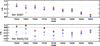 |
Fig. 3 Comparison of equivalent widths (EW) for N iiiλ4097 and λλ4640/42. All atmospheric models calculated with “pseudo line-blanketing” (see text). Black diamonds: results from MH; red triangles: new fastwind calculations with “mixed” N iii ionic model (new level structure, but important transition data from MH); purple squares: new fastwind calculations with new N iii model; blue asterisks: as squares, but DR-contribution to 3d level diminished by a factor of two. Here and in the following, positive and negative EWs refer to absorption and emission lines, respectively. |
First, we test if we are able to reproduce the MH-results for O((f)) and O(f) stars. To this end, we need to invoke (almost) identical conditions, regarding both atmospheric and atomic models. Thus, we modified our N iii ionic model, replacing part of our new data with those used by MH (“mixed” ionic model). In particular, we replaced data for dielectronic recombination (to the three draining levels, 2p2 (2D, 2S,2P), to level 3d, and to few higher important levels – #14, 17, 20 and 21, see Table B.1), the oscillator strengths for the “two electron transitions” (Table 2), and the photoionization cross-sections for all levels below 3d (the cross-sections for the latter did already agree).
Oscillator strengths for the “two electron transition” as used by Mihalas & Hummer (1973) and within our new atomic model.
Consistent with the MH-models, a nitrogen abundance of [N]8 = 8.18 was adopted. This is a factor of 2.5 larger than the solar one, [N⊙] = 7.78 (Asplund et al. 2005)9. To account for the absence of a wind in their models, a negligible mass-loss rate of Ṁ = 10-9 M⊙ yr-1 was used.
Though line-blocking/blanketing could not be included into the atmospheric models in 1973, MH realized its significance and tried to incorporate some important aspect by means of a “pseudo-blanketing” treatment. The N iii photoionization edge (at 261 Å) lies very close to the He ii ground state edge (at 228 Å) in a region of low continuum opacity and high emergent flux (if no line-blocking due to the numerous EUV metal-lines is present), and would cause severe underpopulation of the N iii ground state if the blanketing effect is neglected, as shown by BM71. MH argued that heavy line-blanketing and much lower fluxes are to be expected in this region. To simulate these effects, they extrapolated the He ii ground-state photoionization cross-section beyond the Lyman-edge up to the N iii edge, using a ν-3 extrapolation. To be consistent with their approach, we proceed in the same way by including this treatment into fastwind (see Fig. 6).
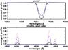 |
Fig. 4 Comparison of fastwind N iii line profiles from model “T3740” with “pseudo line-blanketing”, using different atomic data sets. Solid (black): “mixed” N iii model (see text); dotted (red): new N iii model; dashed (blue): new N iii model, but DR-contribution to 3d level diminished by a factor of two. |
Figure 3 displays the comparison between the resulting equivalent widths from the MH models (black symbols) and our models using the conditions as outlined above (red triangles). Overall, the agreement for λλ4634−4640−4642 is satisfactory10, and slight differences are present only for the hottest models. In agreement with the MH results, our profiles turn from absorption into emission around Teff ~ 37 000 K for dwarfs and at Teff ~ 33 000 K for (super-)giants. As well, the λ4097 line is always in absorption throughout the grid, though our calculations predict moderately more absorption in this line. All lines show the same trend in both sets, and the remaining differences might be attributed to still somewhat different atomic data11.
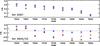 |
Fig. 5 Comparison of equivalent widths (EW) for N iiiλ4097 and λλ4640/42. Diamonds and triangles as Fig. 3. Purple squares: new results using new atomic data and realistic line-blanketing; blue asterisks: as squares, but DR-contribution to 3d level set to zero. |
We note already here that in all cases the emission is more pronounced in low-gravity objects. In high-gravity objects (dwarfs) part of the emission is suppressed because of higher collisional rates ( ∝ ne), driving the relative populations towards LTE.
After demonstrating that we can (almost) reproduce the profiles calculated by MH when similar conditions are applied, the next step is to investigate the effect of the new N iii atomic data implemented during the present work. In fact, this leads to much more triplet emission, see Figs. 3 (purple squares) and 4 (dotted profiles). Even for the coolest models, where MH still obtain weak absorption, our calculations result in strong emission. This big difference is produced by larger DR rates into 3d and a larger drain of 3p by the “two electron transitions”, due to larger oscillator strengths (see Table 2)12. Note also that the λ4097 line becomes weaker, in accordance with the correlation predicted above.
The reaction of the emission strength on the dielectronic data also allows us to check the validity of the implementation of dielectronic recombination by the explicit method, described in Sect. A.1, particularly the dependence on the oscillator strength of the stabilizing transition(s). Figures 3 (blue asterisks) and 4 (dashed) show the reaction of the triplet lines if we diminish the oscillator strength of the strongest stabilizing transition to 3d by a factor of two. This reduction leads to a significantly weaker emission throughout the whole grid, and a slight increase in the absorption strength of λ4097. For a further test on the consistency between implicit and explicit method, see Appendix A.3.
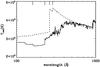 |
Fig. 6 EUV radiation temperatures for model “T3735” with pseudo (dashed) and full (solid) line-blanketing. Important ionization edges are indicated as vertical markers. From left to right: N iv, He ii, N iii (ground-state), and N iii 2p22D. |
5.2. Models with full line-blanketing
In their study, MH could not consider the problem for realistic atmospheres accounting for a consistent description of line-blocking/blanketing, simply because such atmospheric models did not exist at that time. To investigate the differential effect on the N iii emission lines, we calculated the same grid of models, now including full line-blanketing13 as incorporated to fastwind, and compare with the MH calculations (Fig. 5, purple squares vs. black diamonds, respectively).
Astonishingly, the triplet emission almost vanishes throughout the whole grid. This dramatic result points to the importance of including a realistic treatment of line-blanketing when investigating the emission line problem in Of stars. It further implies, of course, that the new mechanism preventing emission in line-blanketed models needs to be understood, and that an alternative explanation/modeling for the observed emission must be found.
Let us first investigate the “inhibition effect”, by considering model “T3735” that displays one of the largest reactions. The most important consequence of the inclusion of line-blocking/blanketing is the decrease of the ionizing fluxes in the EUV. Figure 6 displays corresponding radiation temperatures as a function of wavelength, for the “pseudo line-blanketed”, simple model constructed in analogy to MH (dashed) and the fully line-blanketed model (solid).
Indeed, the presence of substantially different ionizing fluxes around and longward of the N iii edge is the origin of the different triplet emission, via two alternative routes. For part of the cooler models (not the one displayed here), significantly higher radiation temperatures in the N iii continuum (λ < 261 Å) of the “pseudo line-blanketed” models lead to a strong ground-state depopulation. Moreover, the ground-state and the 2p2 levels are strongly collisionally coupled, from the deepest atmosphere to the line-forming region of the photospheric lines. Thus, the ground-state and the 2p2 levels react in a coupled way. If the ground-state becomes depopulated because of a strong radiation field, the 2p2 levels become underpopulated as well, giving rise to a strong drain from level 3p and thus a large source-function for the triplet lines. Corresponding models including a realistic line-blocking (with lower EUV-fluxes) cause much less depopulation of the ground-state and the 2p2 levels, thus suppressing any efficient drain and preventing strong emission in the triplet lines.
For hotter models, e.g., model “T3735” as considered here, the operating effect is vice versa, but leads to the same result. In the simple, MH-like model, the 2p2 levels become strongly depopulated in a direct way, because (i) the ionizing fluxes at the corresponding edges (λ > 261 Å) are extremely high (the ‘pseudo line-blanketing extends “only” until 261 Å); and (ii) because also a strong ionization via doubly excited levels is present, again due to a strong radiation field at the corresponding transition wavelengths around 290–415 Å. Due to the depopulation of the 2p2 levels, the coupled ground-state becomes depopulated as well.
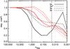 |
Fig. 7 Departure coefficients for important levels regarding the triplet emission, for model “T3735” with pseudo (black) and full (red) line-blanketing (level 2p is the ground-state). The formation region of the triplet lines is indicated by vertical dashed lines. See text. |
On the other hand, the depopulation via direct and “indirect” ionization from 2p2 does not work for consistently blocked models, because of the much lower ionizing fluxes. Insofar, the extension of the He ii ground-state ionization cross section by MH, to mimic the presence of line-blocking, was not sufficient. They should have extrapolated this cross-section at least to the edge of the lowest 2p2 level. In this case, however, they would have found much lower N iii emission, too low to be consistent with observations.
In Fig. 7, we compare the corresponding departure coefficients. Black curves refer to the simple, “pseudo line-blanketed” model, and red curves to the corresponding model with full line-blocking/-blanketing. Obviously, both models display strongly coupled ground and 2p2 states in the formation region of photospheric lines (here: τRoss ≥ 0.02), where these states are much more depopulated in the simple model.
For the conditions discussed so far, a significant depopulation of 2p2 is a prerequisite for obtaining strong emission lines in the optical: only in this case, an efficient drain 3p → 2p2 due to cascading processes can be produced. The consequence of different draining efficiencies becomes obvious if we investigate the run of b3p (dashed). In the pseudo-blanketed model, this level becomes much more depopulated relative to 3d (dashed-dotted), leading to much stronger triplet emission than in the full blanketed model.
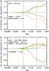 |
Fig. 8 Fractional net rates to and from level 3p (upper panel) and level 3d (lower panel), for model “T3735” with pseudo (red) and full (green) line-blanketing. The formation region of the triplet lines is indicated by vertical dashed lines. |
The impact of the different processes can be examined in detail if we investigate the corresponding net rates responsible for the population and depopulation of level 3p (Fig. 8, upper panel). In this and the following similar plots, we display the dominating individual net rates (i.e., njRji − niRij > 0 for population, with index i the considered level) as a fraction of the total population rate14.
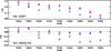 |
Fig. 9 Comparison of equivalent widths for N iiiλ4097 and λλ4640/42. Black diamonds as in Fig. 3 (original results from MH). Other models with [N] = 7.92. Blue asterisks from tlusty (OSTAR2002), red triangles from fastwind, using new atomic data and realistic line-blanketing; purple squares: as triangles, but with temperature and electron stratification from tlusty. For details, see text. |
Indeed, there is a dramatic difference in the net rates that depopulate level 3p via the “two electron” drain (dashed). Whereas for the “pseudo line-blanketed” model the net rate into 2p2 is the dominating one (resulting from the strong depopulation of 2p2), this rate almost vanishes for the model with full line-blanketing. In contrast, the other two important processes, the population by 3d (solid) and the depopulation into 3s (dashed-dotted) are rather similar. Consequently, 3p becomes less depopulated compared to 3d in the fully blanketed models. Moreover, since the (relative) depopulation into 3s remains unaffected, and 3p has a larger population (see Fig. 7), level 3s becomes stronger populated as well. Thus, the blanketed models produce more absorption in λ4097 (cf. Figs. 5 with 3, squares in upper panels).
Since in the older MH-models the triplet emission is also due to the strong population of 3d via DR (Fig. 8, lower panel, red solid), we have to check how the presence of full line-blocking affects this process. In this case, the net-rate from DR (green solid) becomes even negative in part of the line forming region, i.e., the ionization via intermediate doubly excited states partly outweighs the dielectronic recombination. This difference originates from two effects: (i) the photospheric electron densities in the older models are larger, because of missing radiation pressure from metallic lines. Higher electron densities imply higher recombination rates; (ii) in the fully blanketed models, the radiation field at the frequency of the main stabilizing transition to 3d (777 Å) is slightly higher (see Fig. 6), which leads to more ionization. Consequently, DR plays only a minor (or even opposite) role in the fully blocked models, contrasted to the MH case. In the blocked models, the major population is via the 4f level (dashed-dotted). Note also that the Swings mechanism, i.e., a population via the resonance line at 374 Å (dashed), does not play any role in photospheric regions, as already argued by BM71 and shown by MH.
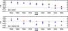 |
Fig. 10 Comparison of equivalent widths (EW) for N iiiλ4097 and λλ4640/42. Black diamonds as in Fig. 3 (results from MH). Red triangles: new results using new atomic data, realistic line-blanketing, no winds; purple rectangles: new results using new atomic data, realistic line-blanketing and winds with a mass-loss rate according to the wind-momentum luminosity relation provided by Repolust et al. (2004); blue asterisks: as purple, but with DR contribution to 3d level set to zero. |
For a final check about the importance of DR to level 3d in models with full line-blanketing, we tested its impact by switching off the main stabilizing transition. From Fig. 5 (blue asterisks), it is obvious that the effect indeed is marginal throughout the whole grid. Thus, a correct treatment of line-blocking seems to suppress both the efficiency of the draining transitions and the dielectronic recombination, and we have to ask ourselves how the observed triplet emission is produced, since the presence of line-blocking cannot be argued away.
Before tackling this problem, in Fig. 9 we compare our results (red triangles) with those from tlusty (Hubeny 1988; Hubeny & Lanz 1995)15 (blue asterisks), as provided by the OSTAR2002 grid16 (Lanz & Hubeny 2003; see also Heap et al. 2006). Contrasted to all other similar plots, we used an abundance of [N] = 7.92, to be consistent with the tlusty grid. Obviously, our fastwind results for the N iii emission lines in dwarfs match exactly those from tlusty, whereas our results for supergiants display somewhat less emission (or more absorption). On the other hand, the absorption line at λ4097 is systematically stronger in all our models, which points to different oscillator strengths. To rule out potential differences in the atmospheric stratification, we calculated an additional grid with temperature and electron structure taken from tlusty, smoothly connected to the wind structure as calculated by fastwind. Corresponding results are displayed by purple squares, and differ hardly from those based on the original fastwind structure, except for model T3233 where the differences in T and ne are larger than elsewhere. The remaining discrepancies for supergiants can be explained by somewhat higher EUV fluxes in the tlusty models, favouring more N iii triplet emission. Nevertheless, the disagreement between fastwind and tlusty is usually much weaker than between these two codes and the results by MH, which underpins our finding that the triplet emission becomes strongly suppressed in fully blanketed models.
5.3. The impact of wind effects
So far, one process has been neglected, namely the (general) presence of winds in OB-stars. Note that MH had not the resources to reproduce O-stars with truly “extended” atmospheres. Regarding their O(f) and O((f)) objects, on the other hand, there was no need to consider wind effects, because the observed N iii triplet emission could be simulated by accounting for DR and “two-electron” drain alone. Actually, MH pointed out that in Of-supergiants (with denser winds) the Swings mechanism could play a crucial role in the overpopulation of 3d: velocity fields are able to shift the resonance lines into the continuum, allowing them to become locally more transparent, and deviations from detailed balance and strong pumping might occur.
With the advent of new atmospheric codes, we are now able to investigate the general role of winds, and to explain how the emission lines are formed within such a scenario. To this end, we have re-calculated the model grid from Table 1, now including the presence of a wind. Prototypical values for terminal velocity and velocity-field exponent have been used, v∞ = 2000 km s-1, β = 0.9, and mass-loss rates were inferred from the wind-momentum luminosity relationship (WLR) provided by Repolust et al. (2004), which differentiates between supergiants and other luminosity classes. Clumping effects have been neglected, but will be discussed in Sect. 8. For a summary of the adopted mass-loss rates, see Table 1.
With the inclusion of winds now, we almost recover the emission predicted in the original MH calculations (Fig. 10). Less emission is produced only for the two hottest models, where the inclusion of a wind has no effect. For all other models, however, the wind effect is large, both for the supergiants and for the dwarfs with a rather low wind-density.
To understand the underlying mechanism, we inspect again the fractional net rates, now for the wind-model “T3735” (Fig. 11). Obviously, the wind induces a significant overpopulation of the 3d level via the ground state rather than the dielectronic recombination, just in the way as indicated above. Due to the velocity field induced Doppler-shifts, the resonance line(s) become desaturated, the rates are no longer in detailed balance, and considerable pumping occurs because of the still quite large radiation field at 374 Å and the significant ground-state population (larger than in the MH-like models). Interestingly, this does not only happen in supergiants, as speculated by MH, but also in dwarfs (at least those with non-negligible mass-loss rate), because the velocity field sets in just in those regions where the emission lines are formed17.
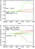 |
Fig. 11 Fractional net rates to and from level 3p (top) and level 3d (bottom), for model “T3735” (full line-blanketing) with no wind (red) and with wind (green). |
The impact of the wind on the population of the 3p level is not as extreme, and the “two electron transition” drain remains as weak as for the wind-free model. Thus, the presence of emission relies mostly on the overpopulation of the 3d level.
Again, we test the (remaining) influence of dielectronic recombination by switching off the stabilizing transition to 3d. Though there is a certain effect, the change is not extreme. Note also that the net rate from dielectronic recombination is larger in the wind model than in the wind-free model, see Fig. 11 (green solid line). Nevertheless, we conclude that dielectronic recombination plays, if at all, only a secondary role in the overpopulation of the 3d level when consistent atmospheric models are considered. The crucial process is pumping by the resonance lines.
The reaction of λ4097 on velocity field effects is more complex. On the one side, there is still the cascade from 3p to 3s, giving rise to a certain correlation. On the other, the resonance line to 3s (at 452 Å) becomes efficient now, and can either feed (as argued in Sect. 2) or drain level 3s, in dependence of its optical depth. Under the conditions discussed here, the resonance line is pumping at cooler temperatures, with a zero net effect on the strength of λ4097 (since the cascade from 3p becomes somewhat decreased, compared to wind-free models). At higher temperatures, the resonance line becomes optically thin18, because of a lower ground-state population, and level 3s can cascade to the ground-state. Thus, the absorption strength of λ4097 might become significantly reduced, which explains, e.g., the strong deviation of model “T4035” from the MH predictions. For this and the hotter models, λ4097 is very weak, and even appears in (very weak) emission for model “T5040”.
6. Comparison with results from cmfgen
In this section, we compare the results from our fastwind models with corresponding ones from cmfgen, a code that is considered to produce highly reliable synthetic spectra, due to its approach of calculating all lines (within its atomic database) in the comoving frame. For this purpose, we used a grid of models for dwarfs and supergiants in the O and early B-star range, which has already been used in previous comparisons (Lenorzer et al. 2004; Puls et al. 2005; Repolust et al. 2005). fastwind models have been calculated with three “explicit” atoms, H, He and our new N atom. Stellar and wind parameters of the grid models are listed in Table 3, with wind parameters following roughly the WLR for Galactic stars. The model designations correspond only coarsely to spectral types and are, with respect to recent calibrations (Repolust et al. 2004; Martins et al. 2005a), somewhat too early. All calculations have been performed with the “old” solar nitrogen abundance, [N] = 7.92 (Grevesse & Sauval 1998), and a micro-turbulence vturb = 15 km s-1.
Stellar and wind parameters of our model grid used to compare synthetic N ii/N iii profiles from fastwind and cmfgen.
For the comparison between fastwind and cmfgen results, we consider useful diagnostic N ii (to check the cooler models) and N iii lines in the blue part of the visual spectrum. Table 4 lists important N iii lines in the range between 4000 to 6500 Å, together with multiplet numbers according to Moore (1975), to provide an impression of how many independent lines are present and which lines belong to the same multiplet19. Additionally, we provide information about adjacent lines present in the spectra of (early) B and O stars, where the major source of contamination arises from O ii and C iii.
This set of lines can be split into five different groups. Lines that belong to the first group (#2, 5, 9–11 in Table 4) are produced by cascade processes of the (doublet) series 1s2 2s2nl with n = 3,4,5 and l = s, p, d, f, g, and additional (over-) population of the 3d level. As outlined in the previous sections, the behavior of these lines is strongly coupled.
The second group (lines #6–8), λλ4510−4514−4518, results from transitions within the quartet system. We consider only the three strongest components of the corresponding multiplet, that are also the least blended ones.
The third group (lines #1, 3, 4) represents three lines, at λλ4003, 4195, and 4200 Å, that are formed between higher lying levels within the doublet system. These lines are weaker than the ones from the previous two groups, but still worth to use them within a comparison of codes and also within a final abundance analysis. Note that N iiiλ4195 and N iiiλ4200 are located within the Stark-wing and the core of He iiλ4200, respectively, which requires a consistent analysis of the total line complex.
Lines at λλ5320, 5327 Å (#12–13) and λλ6445, 6450, 6454, 6467 Å (#14–17) comprise the fourth and fifth group, respectively. The former set of lines is located in a spectral region that is rarely observed, and the latter comprises a multiplet from the quartet system, in the red part of the visual spectrum.
Although most of the lines listed in Table 4 are (usually) visible in not too early O-type spectra, their diagnostic potential for abundance determinations is different. The lines at λλ4510 − 4514 − 4518 (from the quartet system) are certainly the best candidates to infer abundances, since they are quite strong and their formation is rather simple. Also the N iii triplet itself provides valuable information. Due to its complex formation – when in emission – and additional problems (see below and Sect. 7), these lines should be used only as secondary diagnostics, whenever possible. The remaining lines in the blue part of the visual spectrum are rather weak and/or strongly blended with adjacent lines (see Table 4). In particular, the (theoretically) very interesting transition 3p → 3s, N iiiλ4097, is located within the Stark-wing of Hδ. Thus, these lines should be used preferentially as a consistency check, and employed as a direct abundance indicator only at low rotation. Lines in the yellow part of the optical (group four) have not been considered by us so far, since our observational material does not cover this spectral range, and we are not able to judge their diagnostic value for O-type stars. Finally, lines from group five in the red are usually rather weak, and might be used only in high S/N spectra of slowly rotating stars.
Diagnostic N iii lines in the optical, together with adjacent blends.
A detailed comparison between the various N ii (for the later subtypes) and N iii lines from fastwind and cmfgen is provided in Appendix C. Overall, the following trends and problems have been identified.
For models d10v, d8v, and s10a (Figs. C.1–C.3, respectively), the agreement of the N ii lines is almost perfect. For model s8a (Fig. C.4), on the other hand, big discrepancies are found. Most of our lines are much stronger than those from cmfgen, because of the following reason. Within the line-forming region, the electron density as calculated by fastwind is a factor of ≈ 8 higher than the one as calculated by cmfgen, thus enforcing higher recombination rates from N iii to N ii, more N ii and thus stronger lines. This is the only model with such a large discrepancy in the electron density (e.g., the electron densities from models s10a and s6a agree very well), and the reason for this discrepancy needs to be identified in future work. Nevertheless, this discrepancy would not lead to erroneous nitrogen abundances: when analyzing the observations, a prime diagnostic tool are the wings of the hydrogen Balmer lines that react, via Stark-broadening, sensitively on the electron density. After a fit of these wings has been obtained, one can be sure that the electron stratification of the model is reasonable (though the derived gravity might be erroneous then). With a “correct” electron density, however, the abundance determination via N ii should be no further problem.
Let us concentrate now on the N iii lines, beginning with the triplet λλ4634−4640−4642 and accounting for the fact that at cooler temperatures the λ4642 component is dominated by an overlapping O ii line (see Table 4). Except for the dwarf model d6v and the supergiant models s8a and s6a, both codes predict very similar absorption (for the cooler models) and emission lines, thus underpinning the results from our various tests performed in Sect. 5. Interestingly, our emission lines for the hottest dwarfs (d4v and d2v, Figs. C.8 and C.9) are slightly stronger than those predicted by cmfgen, a fact that is not too worrisome accounting for the subtleties involved in the formation process.
What is worrisome, however, is the deviation for models d6v, s8a and s6a (Figs. C.7, C.11 and C.12). Whereas fastwind predicts only slightly refilled absorption profiles for all three models, cmfgen predicts almost completely refilled (i.e., EW ≈ 0) profiles for d6v and s8a, and well developed emission for s6a.
We investigated a number of possible reasons for this discrepancy. At first, the difference in electron density for model s8a (see above) could not explain the strong deviations. At least for our fastwind models, dielectronic recombination does not play any role, and we checked that this is also the case for the cmfgen models, by switching off DR. As it finally turned out, the physical driver that overpopulates the 3d level in cmfgen in the considered parameter range is a coupling with the O iii resonance line at 374 Å, which is discussed in the next section.
With respect to N iiiλ4097, we find a certain trend in the deviation between fastwind and cmfgen absorption profiles. Both for dwarfs and supergiants, our line is weaker at cooler temperatures, similar at intermediate ones and stronger at hotter temperatures.
For N iiiλ4379, the cmfgen models predict more absorption for models with Teff ≤ 35 000 K, because of an overlapping O ii and C iii line. For hotter models, the presence of O ii is no longer important, but there is a still a difference for λ4379, going into emission at the hottest temperatures.
For the quartet multiplet at λλ4510 − 4514 − 4518, we find a similar trend as for λ4097. For dwarfs, the lines are weaker at cooler temperatures, similar at d6v and stronger in absorption at d4v. Likewise then, the emission at d2v is weaker than in cmfgen. For supergiants, the situation is analogous, at least for all models but the hottest one where both codes predict identical emission.
Finally, lines λ4003 and λ4195 (note the blueward Si iii blend at hotter temperatures) show quite a good agreement for both dwarfs and supergiants, with somewhat larger discrepancies only for models d4v and s4a.
In summary, the overall agreement between N ii and N iii profiles as predicted by fastwind and cmfgen is satisfactory, and for most lines and models the differences are not cumbersome. Because of the involved systematics, however, abundance analyses might become slightly biased as a function of temperature, if performed either via fastwind or via cmfgen. Additionally, we have identified also some strong deviations, namely with respect to N ii line-strengths for supergiants around Teff ≈ 30 kK20, and regarding the emission strengths of the N iii triplet, for models d6v, s8a, and s6a.
7. Coupling with O iii
After numerous tests we were finally able to identify the origin of the latter discrepancy. It is the overlap of two resonance lines from O iii and N iii around 374 Å (for details, see Table 5) that is responsible for the stronger emission in cmfgen models compared to the fastwind results. Whereas this process is accounted for in cmfgen, our present fastwind models cannot do so, because oxygen is treated only as a background element, and no exact line transfer (including the overlap) is performed. We note that this is not exactly the Bowen (1935) mechanism as mentioned in Sect. 2, since this mechanism involves also the overlap between another O iii resonance line and the He ii Ly-α line at 303 Å, which does not play a strong role in our cmfgen models as we have convinced ourselves21. Here, only the coupling between N iii and O iii at 374 Å is decisive.
Overlapping N iii and O iii resonance lines around 374 Å.
In the following we discuss some details of the process, by means of the cmfgen model s6a that displays the largest difference to the fastwind predictions. For a further investigation, we “decoupled” N iii from O iii by setting the corresponding oscillator strength of the transition O iii 2p23P2 → 3s 3P to a very low value, and compared the results with those from the “coupled” standard model. Figure 12 shows that the well developed emission lines from the standard models switch into absorption, and become very similar to the corresponding fastwind profiles (Fig. C.12). On the other hand, discarding DR by neglecting the resonances in the photo cross-sections from level 3d had almost no effect on the profiles, in accordance with our previous arguments. (Actually, without resonances there is even more emission than before, which shows that for this model the ionization via doubly excited levels outweighs DR.)
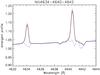 |
Fig. 12 N iiiλλ4634−4640−4642 for three versions of model s6a, as calculated by cmfgen. Solid black: standard version; dotted/red: photo cross-sections for level 3d without resonances (i.e., no DR); dashed/blue: N iii resonance line at 374 Å forbidden to be affected by O iii. For the latter model, the optical triplet lines remain in absorption! |
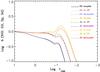 |
Fig. 13 NLTE departure coefficients for three versions of model s6a, as calculated by cmfgen. Lower group of curves: N iii ground state; intermediate group: level 3p, upper group: level 3d. See text. |
Figure 13 displays the corresponding NLTE departure coefficients for the N iii ground state, level 3p and level 3d. Because of the superlevel approach, there is no difference22 between level 3d 2D5/2 (coupled to O iii) and 3d 2D3/2 (not coupled). Whilst the ground state and the 3p level remain similar for all three models (standard, “decoupled” and “coupled’ with resonance-free photo cross-section for 3d), level 3d becomes much stronger overpopulated in the two “coupled” models, compared to the “decoupled” one.
The origin of this stronger overpopulation becomes obvious from Fig. 14. The upper panel displays the source functions of the N iii/O iii resonance lines for the “decoupled” and “coupled” case (again, no difference for individual components, due to the superlevel approach). For the “decoupled” case, the N iii source function is significantly lower than the O iii one, whereas for the “coupled” standard model both source functions are identical, at a level very close to the “decoupled” O iii case. These changes are visualized in the lower panel: because of the line overlap, the N iii source function increases by a factor up to 1.35 (in the line forming region of the optical triplet lines), whereas O iii decreases only marginally.
The source function equality itself results from the strong coupling of the two resonance lines and the fact that both of them are optically thick from the lower wind on, with similar opacities (proportional to the product of cross-section, ionization fraction and abundance)23. It can be shown that the magnitude of the coupled source function mostly depends on those processes that determine the individual source functions in addition to the mean line intensity. This can be easily seen by using the Sobolev approximation, 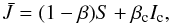 (5)with scattering integral
  , local and core escape probabilities β and βc, and core intensity Ic (Sobolev 1960). In case of overlapping lines, the source function S and the opacities need to account for all components with appropriate weights.
We now assume that the individual source functions (for the packed levels) can be approximated by  (6)where δN and δO correspond to the additional source terms (mostly from cascades to the upper levels), and the well-known factor24 in front of has been approximated by unity.
includes the contributions from all transitions between the fine structure components, =  , exploiting the fact that the reduced occupation numbers for the fine structure levels are equal, ni/gi = nj/gj.
Let us first consider the case of no fine structure splitting, i.e., the overlapping resonance lines should be the only ones connecting the upper and lower levels. Without line overlap, we obtain the well-known result (solving for Eqs. (5) and (6) in parallel) 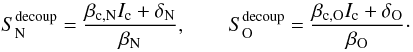 (7)Likewise, but accounting for the line overlap and assuming β ≪ 1 for both components, we find
 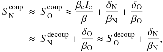 (8)thus, the coupled source functions are larger than in the decoupled case, but (almost) independent on the ratio of their contribution. (In the above equation, the first term of the sum does not depend on any specific opacity as long as the lines – coupled or decoupled – remain optically thick.)
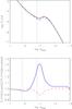 |
Fig. 14 Line source functions for the N iii/O iii resonance lines at 374 Å, for two versions of model s6a, as calculated by cmfgen. Upper panel: N iii “decoupled” (dashed/blue); O iii “decoupled” (dashed-dotted/red); N iii and O iii “coupled” (solid, identical). Lower panel: source function ratios. Solid: N iii (“coupled”)/N iii (“decoupled”); dashed: O iii (“coupled”)/O iii (“decoupled”). The optical triplet lines are formed in the range indicated by the dotted lines. |
For the case of two multiplet lines from both N iii and O iii, with one of each overlapping, the corresponding result for the packed levels reads 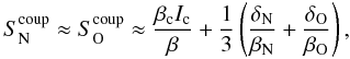 (9)where the escape probabilities βN and βO refer to the total opacity arising from both multiplet lines, and the factor “1/3” can be traced down to the fact that three (optically thick) lines participate in total, two single lines from N iii and O iii, and one coupled line complex.
The corresponding source functions for the decoupled case with packed levels would read 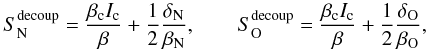 (10)(the factor of two arising from two participating multiplet lines), and a comparison with Eq. (9) shows that in most cases the coupled source function would lie in between the corresponding ones that neglect the line overlap. Again, our result is (almost) independent of the opacity ratio between the overlapping N iii and O iii lines but also independent of the weights of the individual lines within each multiplet25.
Generalization to more multiplet lines is straightforward, and our analytic result compares well to the actual case where the N iii and O iii source functions for the coupled case are identical and lie in between the values for the decoupled situation, see Fig. 14, upper panel.
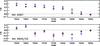 |
Fig. 15 Comparison of equivalent widths (EW) for N iiiλ4097 and λλ4640/42 for models with different nitrogen abundances and wind-strengths. Black diamonds: [N] = 7.78, mass-loss rates as in Table 1. Red triangles: as black diamonds, but with half the mass-loss rate. Purple squares: [N] = 8.18, mass-loss rates as in Table 1. Blue asterisks: as purple squares, but with half the mass-loss rate. All background abundances are solar (Asplund et al. 2005). |
Thus, whenever the source function of the O iiiλ374 line is significantly larger than the one from N iii, a decent effect on the emission strength of the optical triplet lines is to be expected. This situation is particularly met around Teff = 30 to 33 kK, since in this region the upper level of the O iii line is significantly populated by cascades from higher levels.
First test calculations with a simplified oxygen model atom performed by fastwind confirm the general effect, but realistic results cannot be provided before a detailed model atom has been constructed. Let us note, however, that most of the other optical N iii lines are barely affected by the resonance line coupling, and that these lines can be used for diagnostic purposes already now.
In Paper II we derive nitrogen abundances for LMC O-stars from the VLT-FLAMES survey of massive stars. Though there are only few objects in the critical temperature range, at least for one object, N11-029 (O9.7 Ib), we encountered the problem that the observed, refilled N iii triplet (EW ≈ 0) could not be reproduced by fastwind, though with cmfgen. We interpret this problem as due to the resonance line overlap, but stress also the fact that other diagnostic lines enable a satisfactory abundance analysis.
8. Influence of various parameters
Let us finally investigate the influence of important parameters on the strength of the optical emission lines. We stress that the following results have an only qualitative, differential character, as long as the coupling with O iii has not been accounted for, at least in the range Teff ≲ 35 kK.
Nitrogen abundance.
Figure 15 displays the reaction on a variation of nitrogen abundance and mass-loss rate. All models have been calculated with background abundances following Asplund et al. (2005). The (purple) squares correspond (almost, except for the background) to our previous results for [N] = 8.18 (0.4 dex larger than the solar value), and mass-loss rates according to Table 1. Reducing the nitrogen abundance to solar values, [N] = 7.78, results in considerably less emission (black diamonds), which is a consequence of the fact that the relative overpopulation of the 3d level decreases significantly when the formation depth proceeds inwards. The influence on N iiiλ4097, on the other hand, is less extreme, and follows the standard trend that a higher abundance results in stronger absorption lines.
Mass-loss rates.
Also in Fig. 15, asterisks (for [N] = 8.18) and triangles (for [N] = 7.78) correspond to a situation where the mass-loss rates have been decreased, by a factor of two compared to Table 1. Whereas the effect for the enriched models is significant, the models with solar nitrogen abundance are much less affected, though the predicted emission is still much stronger than for models without a wind at all, cf. Fig. 10 (triangles).
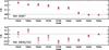 |
Fig. 16 Comparison of equivalent widths (EW) for N iiiλ4097 and λλ4640/42 for models with different background abundances, [N] = 7.78 and mass-loss rates as in Table 1. Black diamonds: Z/Z⊙ = 1.0; red triangles: Z/Z⊙ = 0.5; purple squares: Z/Z⊙ = 0.2. Background abundances scaled to solar abundance pattern from Asplund et al. (2005). |
The origin of this different behaviour is, again, rooted in the specific run of the relative overpopulation of level 3d. For a large nitrogen abundance, the formation takes place in a region where the overpopulation increases quickly with increasing mass-loss rate, whereas for a lower abundance (deeper formation) it remains rather constant over a certain range of formation depths, such that a moderate change in Ṁ has much less effect. Figures 13 and 14 (upper panel), with a formation region corresponding to [N] = 7.92, visualize the general situation (irrespective of whether coupling with O iii is important or not): an increase of the nitrogen abundance shifts the formation depth to the right (towards lower τRoss), where the departure coefficient of level 3d and the source function display a “bump”, due to the large velocity gradient, inducing very strong pumping by the resonance line(s). A decrease of the wind-strength, on the other hand, shifts the position of the bump to the right, while (almost) preserving the formation depth with respect to τRoss. Thus, in case of a large nitrogen abundance the strong overpopulation is lost when Ṁ decreases, leading to a corresponding loss of emission strength. For a lower abundance, however, the formation takes place in a region where the overpopulation displays a “plateau”, and a reduction of Ṁ, i.e., a shift of the bump to the right, has a much weaker effect.
Wind clumping.
Since the N iii emission lines of O-stars are formed in the middle or outer photosphere26, wind clumping has no direct effect on their strength, as long as the photosphere remains unclumped (which is most likely the case, e.g., Puls et al. 2006; Sundqvist et al. 2011; Najarro et al. 2011). Only if the transition region wind/photosphere were clumped, such direct effects are to be expected, due to increased recombination and optically thick clumps affecting the resonance lines (Sundqvist et al. 2011). Indirect effects, however, can be large, since clumpy winds have a lower mass-loss rate than corresponding smooth ones. Since typical Ṁ reductions are expected to be on the order of 2...3 when accounting for micro- and macro-clumping (Sundqvist et al. 2011, and references therein), Fig. 15 (asterisks vs. squares and triangles vs. diamonds) gives also an impression on the expected effects when clumping were in- or excluded in the spectrum synthesis.
Background abundances.
Figure 16 displays the effects when only the background abundances are varied, while, inconsistently, the nitrogen abundance is kept at its solar value and the wind-strengths correspond to the Galactic WLR. Diamonds refer to solar composition, triangles to Z/Z⊙ = 0.5 (roughly LMC) and squares to Z/Z⊙ = 0.2 (roughly SMC). In line with our reasoning from Sect. 5.2, the emission increases significantly when the background abundances decrease, due to reduced line-blocking. Note that for objects with unprocessed nitrogen this effect might be compensated by a lower nitrogen abundance, and, even more, because of lower wind-strengths (Ṁ ∝ (Z/Z⊙)0.7, Mokiem et al. 2007). Note also that the correlation between triplet emission and λ4097 absorption strength has become rather weak, due to the influence of the resonance line connected to level 3s (see Sect. 5.3). Let us finally stress that because of the strong dependence of emission line strength on line-blocking, a sensible assumption on the atmospheric iron abundance is required, due to its dominating effect on the EUV fluxes.
9. Summary and conclusions
In this paper we described the implementation of a nitrogen III model ion into the NLTE atmosphere/spectrum synthesis code fastwind, to allow for future analyses of nitrogen abundances in O-stars27. In particular, we concentrated on a re-investigation of the N iiiλλ4634 − 4640 − 4642 emission line formation. Previous, seminal work by MH has suggested that the formation mechanism of these emission lines in O((f)) and O(f) stars is dominated by two processes: the overpopulation of the 3d level via dielectronic recombination, and the strong drain of the 3p level (towards 2p2) by means of the “two electron transitions”.
To account for the dielectronic recombination process in our new N iii model, we tested two different implementations. Within the implicit method, the contribution of dielectronic recombination is included in the photoionization cross-sections (provided from OPACITY project data), whereas the explicit method uses resonance-free photoionization cross-sections and directly accounts for the different stabilizing transitions from autoionizing levels. Both methods have been implemented into fastwind, and the equivalence of both methods has been shown.
First tests were able to reproduce the results by MH quite well, after adapting our new atomic data to values as used by them. This result was achieved by applying similar assumptions, i.e., wind-free atmospheres and the same approximate treatment of line-blanketing. The triplet emission becomes even increased when using our new atomic data, mostly because of higher oscillator strengths for the “two electron transitions”.
After switching to fully line-blanketed models (still wind-free), however, the situation changes dramatically. Then, the strong emission present in the “pseudo line-blanketed” models is lost (consistent with results from the tlusty OSTAR2002 grid). We have investigated this mechanism in detail, and shown that it is rooted in the overall lower ionizing EUV-fluxes (not only until the N iii edge as assumed by MH), either directly or indirectly, and the strong collisional coupling of the ground state and the 2p2 levels. In any case, these levels become much less underpopulated in fully line-blanketed models, thus preventing an effective drain of the 3p level. We also questioned the role of dielectronic recombination regarding the overpopulation of the 3d level. After setting the DR contribution to the 3d level to zero, almost no reaction on the triplet lines was found throughout the whole model grid. Both results lead to the conclusion that, under realistic conditions of line-blocking/-blanketing with solar background abundances, both the drain and the dielectronic recombination lose their key role as assigned to them by MH.
This key role is now played by the stellar wind. Already MH suggested that the emission lines of Of stars (contrasted to O((f)) and O(f) stars) might be formed due to the Swings (1948) mechanism, an overpopulation of the 3d level by pumping through the corresponding resonance line in an “extended atmosphere”. This suggestion could not be proven though, since MH had not the tools to model such atmospheres. Nowadays, this is no longer a problem, and when we include the wind in our calculations (with mass-loss rates following the “unclumped” Galactic WLR), it turns out that we obtain almost the identical emission as present in the original MH simulations (performed without wind and without realistic line-blanketing). By inspection of the net rates into and from the 3d level, we noticed how the wind induces the overpopulation of the 3d level via pumping from the ground state rather than by dielectronic recombination. A prerequisite of this process is that the wind-strength is large enough to display a significantly accelerating velocity field already in the photospheric formation region of the triplet lines, to allow the resonance lines to leave detailed balance.
The most important implication of our study is that under Galactic conditions DR plays only a secondary role, both for O-stars with “compact” and with “extended” atmospheres, whereas the key process is the overpopulation due to the resonance line in the presence of an accelerating velocity field. Note that without such a velocity field the resonance line loses its impact though. Consequently, it is to be expected that hydrostatic NLTE codes, such as tlusty and detail/surface, will not be suited to quantitatively synthesize the N iii triplet lines (and, to a lesser extent, also N iiiλ4097, because of their interrelation), unless the wind-strength is significantly below the Galactic WLR or the background metallicity, Z, is much lower than the Galactic one (see Heap et al. 2006, who performed nitrogen diagnostics for SMC O-stars by means of tlusty). Note also that our results have been derived for O-star conditions only, and should be valid as long as the N iii emission lines, to a major extent, are formed in the photosphere or in the transition region. For objects with significantly denser winds, e.g., WN-stars, our analysis would certainly need to be extended, since additional effects might be present or might even dominate.
In order to check our new model atom and the predictive power of fastwind, we performed first comparisons with results from the alternative model atmosphere code cmfgen, for a small grid of O-type dwarfs and supergiants. For this objective we used a set of important N ii and N iii lines in the blue part of the visual spectrum. The overall agreement between both codes is mostly satisfactory, though some systematic deviations demand a further clarification in terms of a comparison with observations.
Within the range 30 000 K ≤ Teff ≤ 35 000 K, however, some major discrepancies have been found. Here, cmfgen triggers the emission at λλ4634 − 4640 − 4642 earlier, i.e., at cooler temperatures, than calculations from fastwind. This effect could be traced down to the overlap of the N iii resonance line (actually, one of its fine-structure components, at 374.43 Å) with a resonance line from O iii, which is of similar strength throughout the O-star domain. We studied this effect by means of the corresponding cmfgen calculations (since fastwind lacks a detailed O iii model), and also by analytic considerations.
As long as both resonance lines are optically thick, source function equality is achieved. Under most conditions, the “coupled” source function lies in between the individual, “decoupled” ones from N iii and O iii. In the critical temperature range now, the decoupled O iii source function is predicted to be much larger than the N iii one (due to substantial cascades from upper levels), and leads, after being coupled with N iii, to significant values for the combined source function, beyond the decoupled N iii case. Thus, the important 3d level becomes more pumped, and the triplet emission occurs at cooler temperatures than without coupling. When the coupling is neglected in cmfgen, the predicted triplet emission vanishes and the profiles become similar to those from fastwind.
It might be suspected that the impact of the O iii resonance line overlap introduces an additional parameter to be known when the nitrogen abundance shall be determined via the triplet lines, namely the oxygen abundance. As we have shown by our analytic considerations, however, this parameter remains rather unimportant28 as long as both resonance lines are optically thick, which is true in the interesting parameter range. We have tested this prediction by lowering the O iii oscillator strength in cmfgen by a large factor (50), and found no difference in the coupled source function and triplet emission.
Summarizing, not only the N iii resonance line itself is responsible for the (strong) triplet emission, but also the overlapping O iii resonance line, at least at later O-types. Indeed, for one corresponding object studied in Paper II, N11-029 (O9.7 Ib), we encountered the problem that the observed N iii triplet could not be reproduced by fastwind, though with cmfgen, and we interpreted this problem as due to the resonance line overlap. Insofar, we need to incorporate this process into fastwind if we aim at deriving nitrogen abundances at cooler temperatures from the triplet lines alone. Fortunately, the contamination of the other optical lines by this process remains weak, so that these lines can be used already now, and the nitrogen abundance determination by fastwind is not hindered.
Our study implies two important consequences that need to be tested in future comparisons with observations.
-
(i)
Since the efficiency of DR and “two electron”drain is strongly dependent on the degree of line-blanketing/-blocking, we predict that in a metal-poorenvironment (e.g., in the Small Magellanic Cloud withZ/Z⊙ ≈ 0.2) the emission becomes stronger again, due to less EUV line-blocking. On the other hand, in such a low-Z environment also the wind-strengths and the base-line nitrogen abundance become lower, and the combined effects need to be investigated in detail.
-
(ii)
As outlined above, the triplet lines from O-type stars are of photospheric origin and depend, via the N iii (and O iii) resonance lines, on the actual wind-strength (independent of clumping and X-ray properties), determining the onset of the accelerating velocity field. Thus, their emission strengths might be used to constrain the stellar mass-loss rate (after the line-formation has been shown to work reliably), if the nitrogen abundance can be derived independently from other lines. In particular, “weak-winded” stars (e.g., Bouret et al. 2003; Martins et al. 2005b; Puls et al. 2008; Marcolino et al. 2009; Najarro et al. 2011) have a rather weak wind for their luminosity, being a factor of 10 to 100 thinner than predicted/observed for their counterparts with “normal” winds. Thus, it might be suspected that weak-winded stars display much less emission than stars with “normal” winds of similar type. This requires, that a) there are weak-winded stars also at intermediate O-types, and b) that the winds of their “normal” counterparts are not strongly clumped, which would diminish also their emission because of lower-than-thought mass-loss rates. Using the N iii triplet as an independent mass-loss diagnostics would be somewhat similar to the corresponding application of the NIR Brα-line (Najarro et al. 2011; see also Puls et al. 2008), but with the advantage that the emission strength of the triplet is a rather monotonic function of Ṁ, whereas Brα changes its behaviour from weak to normal winds considerably.
Online material
Appendix A: Dielectronic recombination: implementation to fastwind
In the present work we implemented dielectronic recombination into fastwind, which, so far, could not (or only approximately) deal with this process. To this end, new rates (both for the dielectronic recombination and for the inverse process) had to be inserted into the system of the rate equations.
A.1. Explicit method
To calculate these rates for the “explicit method” (see Sect. 3.2), we follow the formulation as provided by Nussbaumer & Storey (1983). In compact notation, the dielectronic recombination for an element X and charge m + 1 proceeds via 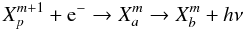 (A.1)where p is a parent state of the m + 1 times ionized element X, a is an autoionizing state and b is a bound state. We denote the initial state of expression A.1, composed of the recombining ion and the free electron, as a continuum state c. We refer to the first process as dielectronic capture and to its inverse as autoionization. In general, dielectronic captures and autoionizations link state a to a large number of continuum states c.
As a final result29, Nussbaumer & Storey (1983) could express the dielectronic recombination coefficient between autoionizing state a and bound state j, αDR(aj), as 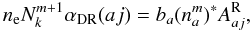 (A.2)with
  the corresponding radiative transition probability for the stabilizing transition (Einstein coefficient for spontaneous emission, corrections for induced emission will be applied below), total ion density
  (element k),
  the LTE population of state a with respect to the actual (NLTE) ground-state population of the next higher ion and the actual electron density, and ba the related NLTE departure coefficient.
The last quantity can be expressed in terms of (i) the autoionization coefficient(s),  , between state a and all possible compound-states c that can form a, (ii) the radiative transition probabilities,
  , between state a and all possible bound and autoionizing states with lower energy i to which state a can decay, and (iii) the departure coefficients of the contributing parent levels, bp (here with respect to the ground-state of the same ion,
  )
) 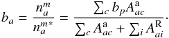 (A.3)Usually, the autoionizing probabilities for state a are much larger than the radiative probabilities for decay, and often there is only one parent level, namely the ground-state of ion m + 1,
  , i.e., bp = 1. Under these conditions (which are similar for excited parent levels assumed to be in LTE with respect to the ground level), ba → 1, and the dielectronic rate depends only on the LTE population of state a and the radiative transition probability . All dependencies on the autoionization probabilities have “vanished”, and we need only the value of that can be derived from the Saha-equation and the ground-state population of ion m + 1, without including the autoionizing levels into the rate equations.
In stellar atmospheres, one needs (in addition to the spontaneous emission to level j) to account for stimulated emission as well, i.e., 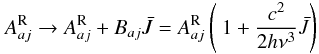 (A.4)with Baj the Einstein coefficient for stimulated emission and
  the scattering integral (profile weighted, frequency integrated mean intensity) for the stabilizing transition. Since the important resonances are broad, the scattering integrals might be replaced by the mean intensities, Jν, of the pseudo-continuum (i.e., including all background opacities/emissivities) at the frequency of the stabilizing line.
Finally, we can define the total dielectronic rate to level j from any possible autoionizing state ai, 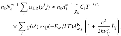 (A.5)which might need to be augmented by departure coefficients bai inside the rhs sum if the parent levels are not the ground-state or not in LTE with respect to the ground-state. The inverse upward rate involves only the line process(es),
 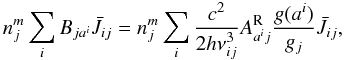 (A.6)with Bji the Einstein-coefficient(s) for absorption. It is easy to show that for LTE conditions (
 and Planckian radiation in the lines) the upward and downward rates cancel each other exactly, as required for thermalization.
Though we have followed here the derivation by Nussbaumer & Storey (1983), our final results for the downward and upward rates are identical with the formulation as used by Mihalas & Hummer (1973) in their investigation.
These rates have been implemented into fastwind and are used whenever the “explicit method” is applied. The only input parameters that need to be specified in the atomic data input file are the transition frequencies and the oscillator-strengths for the stabilizing lines, fja, which relate to the products  via
via 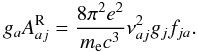 (A.7)For convenience and for consistency with the formulation of “normal” recombination rates (see Sect. A.2), the quantity is expressed in terms of the LTE-population (with respect to actual ionization conditions) of the lower, stabilizing level
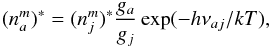 (A.8)so that the downward rate (for a specific autoionizing level a) can be expressed as
 ![Mathematical equation: \appendix \setcounter{section}{1} \begin{eqnarray} \label{dr-rate-final} n_{\rm e} N_k^{m+1} \alpha_{\rm DR}(aj) & = & [b_a] (n_j^m)^{*} \frac{8 \pi^2 e^2}{m_{\rm e} c^3} \nu_{aj}^2 f_{ja} \exp(-h\nu_{aj}/kT) \nonumber \\ & &\times \left( 1 + \frac{c^2}{2h \nu_{aj}^3} \bar{J}_{aj} \right). \end{eqnarray}](/articles/aa/full_html/2011/12/aa17101-11/aa17101-11-eq157.png) (A.9)Summation over all contributing autoionizing states yields the final rate.
(A.9)Summation over all contributing autoionizing states yields the final rate.
In this explicit method, the rates for dielectronic recombinations and inverse processes are calculated in a separate step and then added to the rates involving resonance-free photoionization cross-sections alone. In our model ion (Sect. 4), we use such cross-sections defined in terms of the Seaton approximation (Eq. (4)), which, together with the data for the stabilizing transitions, have been taken from the wm-basic atomic database. Note that we consider processes both from/to ground-states as well as from/to excited states within ion m + 1, so far on the assumption that the autoionizing levels are in LTE (i.e., without including these levels into the model atom and rate equations).
A.2. Implicit method
Within the implicit method, the DR contribution is already contained within the “conventional” recombination rates, (nj/nk)∗Rkj, to yield a total number of recombinations 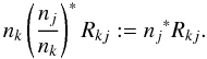 (A.10)As usual, nk is the actual population of the recombining ion in state k and (nj/nk) ∗ the LTE population ratio of the considered level to which the process recombines (either directly or via the intermediate doubly excited state). Rkj is defined as
 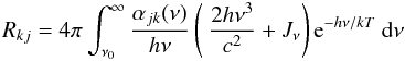 (A.11)with mean intensity Jν and total photoionization cross-section (including resonances), αjk(ν).
In the following, we show that this formulation is consistent with the rates derived in Sect. A.1. We split the cross-section into a resonance-free contribution, and a contribution from the resonances, 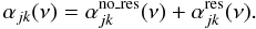 (A.12)The total recombination rate is then the sum of direct and dielectronic recombination,
 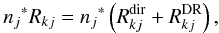 (A.13)with
 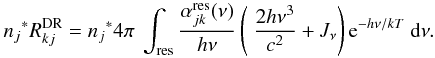 (A.14)The resonances are narrow enough so that most of the frequency dependent quantities can be drawn in front of the integral, evaluated at the average position of the resonances i,
 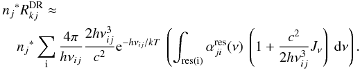 (A.15)The integral over the cross-sections of the resonances corresponds to the cross-section of the stabilizing transitions,
 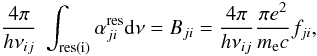 (A.16)with Einstein-coefficient Bji and oscillator-strength fji. Likewise,
 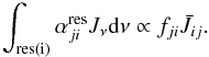 Then, indeed, we recover the result from Eq. (A.9) (explicit formulation),
 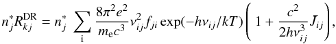 (A.17)if, as outlined in Sect. A.1, the autoionizing levels are in or close to LTE. Note that this is a necessary condition for the implicit method to yield reliable results30, otherwise one has to use exclusively the explicit approach and to include the autoionizing levels into the model atom and rate equations.
The proof that the rates for the inverse photoionization process, calculated either by the implicit method (using total photoionization cross-sections) or via rates from resonance-free cross-sections plus rates involving the excitation of the second electron, are consistent, is analogous and omitted here.
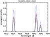 |
Fig. A.1 Consistency of implicit and explicit method. Comparison of N iiiλλ4634 − 4640 − 4642 profiles from model “T3740”, for calculations using a different treatment of DR to the 3d level. Implicit method (solid/black), explicit method (dotted/red), explicit method with oscillator strength for the stabilizing transition increased (dashed/blue) and decreased (dashed-dotted/black) by a factor of two. |
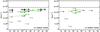 |
Fig. B.1 Grotrian diagrams for the N iii doublet (left) and quartet (right) system. Level numbers refer to Table B.1. Levels # 8, 10, 11 refer to the 3s, 3p and 3d levels involved in the formation of N iiiλλ4634 − 4640 − 4642, and # 3, 4, 5 refer to levels 2p2 (2D, 2S, 2P) that drain level 3p via “two electron transitions”. Important optical transitions are indicated by green lines and numbers referring to Table 4 in the main section. |
A.3. Consistency check
To check the consistency of our implementation of implicit and explicit DR treatment, we carried out the following test. First, to ensure consistent data, we derived the oscillator strength corresponding to the wide PEC resonance in the total photoionization cross-section (Fig. 2) by integrating over the cross-section and applying Eq. (A.16)31. The resulting value (f = 0.45, which is somewhat smaller than the data provided by the wm-basic database, f = 0.60) was then used within the explicit method, at the original wavelength (which coincides with the position of the resonance). As displayed in Fig. A.1 for the case of model “T3740” with “pseudo line-blanketing” (see Sect. 5.1), both methods result in very similar line profiles for the N iii emission triplet, proving their consistency. Figure A.1 also displays the strong reaction of the N iii triplet when the oscillator strength is either increased or diminished by a factor of two.
Appendix B: Details on the N iii model ion
Table B.1 displays the electronic configurations and term designations of our N iii ionic model, and Fig. B.1 the corresponding Grotrian diagrams for the doublet and the quartet systems, indicating important diagnostic transitions in the optical (cf. Sect. 6).
Appendix C: Comparison of line profiles with results from cmfgen
In this appendix, we display a comparison of N iii (and partly N ii) line profiles from fastwind (black) and cmfgen (green), for all models from the grid presented in Table 3. For a discussion, see Sect. 6.
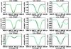 |
Fig. C.1 Comparison of N ii line profiles from present work (black) and cmfgen (green), for model d10v (for parameters, see Table 3). |
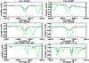 |
Fig. C.5 Comparison of N iii line profiles from present work (black) and cmfgen (green), for model d10v. |
Due to a rapid achievement of the CN equilibrium, whilst the oxygen depletion implied by the full CNO equilibrium is only found in rapidly rotating and more massive stars at later stages, e.g., Brott et al. (2011a).
Baseline abundances for all three environments from H ii regions and unevolved B-stars, see Hunter et al. (2007).
This will almost always be the case, otherwise the states are more or less bound.
When calculating the final synthetic profiles we use, when necessary, the un-packed levels by assuming that ni/gi – with occupation number ni and statistical weight gi – is similar for each sub-level within a packed level, due to strong collisional coupling.
http://www.nist.gov/physlab/data/asd.cfm, firstly described in Kelleher et al. (1999).
See Pauldrach et al. (1994). In brief, the atomic structure code superstructure (Eissner & Nussbaumer 1969; Eissner 1991) has been used to calculate all bound state energies in LS and intermediate coupling as well as related atomic data, particularly oscillator strengths including those for stabilizing transitions.
[A] = log A/H + 12, with A/H the number density of element A with respect to hydrogen.
Asplund et al. (2009) provide a slightly larger value, [N⊙] = 7.83 ± 0.05, where this difference is irrelevant in the following context.
Here and in the following, we only display the total equivalent widths of the λλ4640/4642 components; the behavior of λ4634 is analogous.
Number of levels, collisional data and LTE assumption concerning the quartet system levels by MH.
A similar effect has already been noted by MH when they increased the corresponding oscillator strengths in their atomic model.
Using background metallicities corresponding to the “older” solar abundances from Grevesse & Sauval (1998), but keeping [N] = 8.18.
Which in statistical equilibrium is identical to the total depopulation rate.
A code that assumes plane-parallel geometry, hydrostatic and radiative equilibrium, and calculates line-blanketed NLTE model atmospheres and corresponding synthetic profiles. Due to its restrictions, only objects with negligible winds can be analyzed.
Equivalent widths from own integration.
An analogous desaturation through velocity field induced Doppler shifts in stars with low mass loss rates was found by Najarro et al. (1996) in the He i resonance lines of B giants.
Note that the oscillator strength is more than a factor of 10 lower than that of the resonance line feeding 3d.
A similar table regarding N ii, N iv and N v lines will be presented in Paper II.
Rooted within a different stratification of electron density.
Insofar, the O iii lines at λλ3340, 3444, 3759 mentioned in Sect. 2 remain in absorption.
Assumed to be balanced by collisions.
In the formation region of the optical lines, the opacity ratio between the N iii and O iii resonance lines ranges from roughly 5 for the coolest models to 0.5 for the hottest ones.
Corresponding to (1-ε) in a two-level atom, with ε roughly the ratio of collisional to spontaneous radiative rate coefficient, for the downward transition.
As long as β ≪ 1.
Only for a very large nitrogen abundance or mass-loss rate, (“slash stars” or Wolf-Rayets) the formation takes place in the wind.
Corresponding N ii/N iv/N v model ions will be presented in Paper II.
Except for certain differences in the EUV-fluxes etc.
See also Mihalas (1978) for a simplified derivation.
Which has been used to calculate the total cross-sections as provided by, e.g., the OPACITY Project.
Of course, the underlying contribution responsible for direct ionization needs to be subtracted.
Acknowledgments
We thank our anonymous referee for valuable comments and suggestions. J.G.R.G. gratefully acknowledges financial support from the German DFG, under grant 418 SPA 112/1/08 (agreement between the DFG and the Instituto de Astrofisica de Canarias), and J.P and F.N. acknowledge financial support from the Spanish Ministerio de Ciencia e Innovación under projects AYA2008-06166-C03-02 and AYA2010-21697-C05-01. Many thanks to John Hillier for providing the cmfgen code, and particularly to Keith Butler for his advice and help on the nitrogen atomic data and useful suggestions on the manuscript.
References
- Allen, C. W. 1973, Astrophysical quantities, 3rd edn. (London: University of London, Athlone Press) [Google Scholar]
- Asplund, M., Grevesse, N., & Sauval, A. J. 2005, in Cosmic Abundances as Records of Stellar Evolution and Nucleosynthesis, ed. T. G. Barnes III, & F. N. Bash, ASP Conf. Ser., 336, 25 [Google Scholar]
- Asplund, M., Grevesse, N., Sauval, A. J., & Scott, P. 2009, ARA&A, 47, 481 [NASA ADS] [CrossRef] [Google Scholar]
- Bautista, M. A., Romano, P., & Pradhan, A. K. 1998, ApJS, 118, 259 [NASA ADS] [CrossRef] [Google Scholar]
- Bell, K. L., Hibbert, A., Stafford, R. P., & Brage, T. 1995, MNRAS, 272, 909 [NASA ADS] [Google Scholar]
- Berrington, K. A., Burke, P. G., Butler, K., et al. 1987, J. Phys. B At. Mol. Phys., 20, 6379 [NASA ADS] [CrossRef] [Google Scholar]
- Bouret, J.-C., Lanz, T., Hillier, D. J., et al. 2003, ApJ, 595, 1182 [NASA ADS] [CrossRef] [Google Scholar]
- Bowen, I. S. 1935, ApJ, 81, 1 [NASA ADS] [CrossRef] [Google Scholar]
- Brott, I., de Mink, S. E., Cantiello, M., et al. 2011a, A&A, 530, A115 [NASA ADS] [CrossRef] [EDP Sciences] [Google Scholar]
- Brott, I., Evans, C. J., Hunter, I., et al. 2011b, A&A, 530, A116 [NASA ADS] [CrossRef] [EDP Sciences] [Google Scholar]
- Bruccato, R. J., & Mihalas, D. 1971, MNRAS, 154, 491 [NASA ADS] [Google Scholar]
- Cunto, W., & Mendoza, C. 1992, Rev. Mex. Astron. Astrofis., 23, 107 [NASA ADS] [Google Scholar]
- Eissner, W. 1991, J. Phys. IV (France), 1, C1 [Google Scholar]
- Eissner, W., & Nussbaumer, H. 1969, in Premiere Reunion de l’Association Europeene de Spectroscopie Atomique No. 42 (Paris-Orsay: Faculté des Sciences) [Google Scholar]
- Evans, C. J., Lennon, D. J., Smartt, S. J., & Trundle, C. 2006, A&A, 456, 623 [NASA ADS] [CrossRef] [EDP Sciences] [Google Scholar]
- Evans, C. J., Taylor, W. D., Hénault-Brunet, V., et al. 2011, A&A, 530, A108 [NASA ADS] [CrossRef] [EDP Sciences] [Google Scholar]
- Fernley, J. A., Hibbert, A., Kingston, A. E., & Seaton, M. J. 1999, J. Phys. B At. Mol. Phys., 32, 5507 [NASA ADS] [CrossRef] [Google Scholar]
- Grevesse, N., & Sauval, A. J. 1998, Space Sci. Rev., 85, 161 [NASA ADS] [CrossRef] [Google Scholar]
- Heap, S. R., Lanz, T., & Hubeny, I. 2006, ApJ, 638, 409 [NASA ADS] [CrossRef] [Google Scholar]
- Heger, A., & Langer, N. 2000, ApJ, 544, 1016 [NASA ADS] [CrossRef] [Google Scholar]
- Hillier, D. J., & Miller, D. L. 1998, ApJ, 496, 407 [NASA ADS] [CrossRef] [Google Scholar]
- Hillier, D. J., Lanz, T., Heap, S. R., et al. 2003, ApJ, 588, 1039 [NASA ADS] [CrossRef] [Google Scholar]
- Howarth, I. D., Siebert, K. W., Hussain, G. A. J., & Prinja, R. K. 1997, MNRAS, 284, 265 [NASA ADS] [CrossRef] [Google Scholar]
- Hubeny, I. 1988, Comp. Phys. Comm., 52, 103 [Google Scholar]
- Hubeny, I., & Lanz, T. 1995, ApJ, 439, 875 [Google Scholar]
- Hunter, I., Dufton, P. L., Smartt, S. J., et al. 2007, A&A, 466, 277 [NASA ADS] [CrossRef] [EDP Sciences] [Google Scholar]
- Hunter, I., Brott, I., Lennon, D. J., et al. 2008, ApJ, 676, L29 [NASA ADS] [CrossRef] [Google Scholar]
- Hunter, I., Brott, I., Langer, N., et al. 2009a, A&A, 496, 841 [NASA ADS] [CrossRef] [EDP Sciences] [Google Scholar]
- Hunter, I., Lennon, D. J., Dufton, P. L., et al. 2009b, A&A, 504, 211 [NASA ADS] [CrossRef] [EDP Sciences] [Google Scholar]
- Kelleher, D. E., Mohr, P. J., Martin, W. C., et al. 1999, in SPIE Conf. Ser. 3818, ed. G. R. Carruthers, & K. F. Dymond, 170 [Google Scholar]
- Lanz, T., & Hubeny, I. 2003, ApJS, 146, 417 [NASA ADS] [CrossRef] [Google Scholar]
- Lenorzer, A., Mokiem, M. R., de Koter, A., & Puls, J. 2004, A&A, 422, 275 [NASA ADS] [CrossRef] [EDP Sciences] [Google Scholar]
- Marcolino, W. L. F., Bouret, J., Martins, F., et al. 2009, A&A, 498, 837 [NASA ADS] [CrossRef] [EDP Sciences] [Google Scholar]
- Markova, N., & Puls, J. 2008, A&A, 478, 823 [NASA ADS] [CrossRef] [EDP Sciences] [Google Scholar]
- Martins, F., Schaerer, D., & Hillier, D. J. 2005a, A&A, 436, 1049 [NASA ADS] [CrossRef] [EDP Sciences] [Google Scholar]
- Martins, F., Schaerer, D., Hillier, D. J., et al. 2005b, A&A, 441, 735 [NASA ADS] [CrossRef] [EDP Sciences] [Google Scholar]
- Meynet, G., & Maeder, A. 2000, A&A, 361, 101 [NASA ADS] [Google Scholar]
- Mihalas, D. 1971, ApJ, 170, 541 [NASA ADS] [CrossRef] [Google Scholar]
- Mihalas, D. 1978, Stellar atmospheres, 2nd edn. (San Francisco: W. H. Freeman and Co.) [Google Scholar]
- Mihalas, D., & Hummer, D. G. 1973, ApJ, 179, 827 [NASA ADS] [CrossRef] [Google Scholar]
- Mokiem, M. R., de Koter, A., Vink, J. S., et al. 2007, A&A, 473, 603 [NASA ADS] [CrossRef] [EDP Sciences] [Google Scholar]
- Moore, C. E. 1975, Selected tables of atomic spectra – A: Atomic energy levels, second edition, B: Multiplet table, N I, N II, N III, Data derived from the analyses of optical spectra, ed. C. E. Moore [Google Scholar]
- Najarro, F., Kudritzki, R. P., Cassinelli, J. P., Stahl, O., & Hillier, D. J. 1996, A&A, 306, 892 [NASA ADS] [Google Scholar]
- Najarro, F., Hanson, M. M., & Puls, J. 2011, A&A, 535, A32 [NASA ADS] [CrossRef] [EDP Sciences] [Google Scholar]
- Nikitin, A. A., & Yakubovskii, O. A. 1963, SvA, 7, 189 [NASA ADS] [Google Scholar]
- Nussbaumer, H., & Storey, P. J. 1983, A&A, 126, 75 [NASA ADS] [Google Scholar]
- Oke, J. B. 1954, ApJ, 120, 22 [NASA ADS] [CrossRef] [Google Scholar]
- Pauldrach, A. W. A., & Puls, J. 1990, A&A, 237, 409 [NASA ADS] [Google Scholar]
- Pauldrach, A. W. A., Kudritzki, R. P., Puls, J., Butler, K., & Hunsinger, J. 1994, A&A, 283, 525 [Google Scholar]
- Pauldrach, A. W. A., Hoffmann, T. L., & Lennon, M. 2001, A&A, 375, 161 [NASA ADS] [CrossRef] [EDP Sciences] [Google Scholar]
- Puls, J., Urbaneja, M. A., Venero, R., et al. 2005, A&A, 435, 669 [NASA ADS] [CrossRef] [EDP Sciences] [Google Scholar]
- Puls, J., Markova, N., Scuderi, S., et al. 2006, A&A, 454, 625 [NASA ADS] [CrossRef] [EDP Sciences] [Google Scholar]
- Puls, J., Vink, J. S., & Najarro, F. 2008, A&ARv, 16, 209 [NASA ADS] [CrossRef] [EDP Sciences] [Google Scholar]
- Puls, J., Sundqvist, J. O., & Rivero González, J. G. 2010, in Active OB stars: structure, evolution, mass-loss & critical limits, ed. C. Neiner, G. Wade, G. Meynet, & G. Peters (Cambridge Univ. Press), IAU Symp., 272 [Google Scholar]
- Repolust, T., Puls, J., & Herrero, A. 2004, A&A, 415, 349 [NASA ADS] [CrossRef] [EDP Sciences] [Google Scholar]
- Repolust, T., Puls, J., Hanson, M. M., Kudritzki, R.-P., & Mokiem, M. R. 2005, A&A, 440, 261 [NASA ADS] [CrossRef] [EDP Sciences] [Google Scholar]
- Seaton, M. J. 1958, MNRAS, 118, 504 [NASA ADS] [CrossRef] [Google Scholar]
- Seaton, M. J. 1962, in Atomic and Molecular Processes, ed. D. R. Bates (New York: Academic Press), 375 [Google Scholar]
- Sobolev, V. V. 1960, Moving envelopes of stars (Cambridge: Harvard University Press) [Google Scholar]
- Sota, A., Maíz Apellániz, J., Walborn, N. R., et al. 2011, ApJS, 193, 24 [NASA ADS] [CrossRef] [Google Scholar]
- Stafford, R. P., Bell, K. L., & Hibbert, A. 1994, MNRAS, 266, 715 [NASA ADS] [CrossRef] [Google Scholar]
- Sundqvist, J. O., Puls, J., Feldmeier, A., & Owocki, S. P. 2011, A&A, 528, A64 [NASA ADS] [CrossRef] [EDP Sciences] [Google Scholar]
- Swings, P. 1948, Ann. Astrophys., 11, 228 [Google Scholar]
- Swings, P., & Struve, O. 1940, ApJ, 91, 546 [NASA ADS] [CrossRef] [Google Scholar]
- van Regemorter, H. 1962, ApJ, 136, 906 [NASA ADS] [CrossRef] [Google Scholar]
- Vink, J. S., de Koter, A., & Lamers, H. J. G. L. M. 2000, A&A, 362, 295 [NASA ADS] [Google Scholar]
- Vink, J. S., Brott, I., Gräfener, G., et al. 2010, A&A, 512, L7 [NASA ADS] [CrossRef] [EDP Sciences] [Google Scholar]
- Walborn, N. R. 1971, ApJS, 23, 257 [NASA ADS] [CrossRef] [Google Scholar]
- Walborn, N. R., Morrell, N. I., Howarth, I. D., et al. 2004, ApJ, 608, 1028 [NASA ADS] [CrossRef] [Google Scholar]
- Yan, Y., & Seaton, M. J. 1987, J. Phys. B At. Mol. Phys., 20, 6409 [NASA ADS] [CrossRef] [Google Scholar]
All Tables
Oscillator strengths for the “two electron transition” as used by Mihalas & Hummer (1973) and within our new atomic model.
Stellar and wind parameters of our model grid used to compare synthetic N ii/N iii profiles from fastwind and cmfgen.
All Figures
|
Fig. 1 Grotrian diagram displaying the transitions involved in the N iii emission lines problem. The horizontal line marks the N iii ionization threshold. The N iiiλλ4634 − 4640 − 4642 triplet is formed by the transitions 3d → 3p, while the absorption lines at λλ4097-4103 are due to the transitions 3p → 3s. An effective drain of 3p is provided by the “two electron transitions” 3p → 2p |
| In the text | |
|
Fig. 2 Comparison of the “raw” cross-section from the OPACITY project (black), and the smoothed one (grey/blue), for the 3d 2D state of N iii. Note the numerous complex resonances. An example for a PEC resonance, being much broader than the usual Rydberg resonances, is marked by the vertical arrow. Dashed: corresponding resonance-free data in terms of the Seaton (1958) approximation from wm-basic. |
| In the text | |
|
Fig. 3 Comparison of equivalent widths (EW) for N iiiλ4097 and λλ4640/42. All atmospheric models calculated with “pseudo line-blanketing” (see text). Black diamonds: results from MH; red triangles: new fastwind calculations with “mixed” N iii ionic model (new level structure, but important transition data from MH); purple squares: new fastwind calculations with new N iii model; blue asterisks: as squares, but DR-contribution to 3d level diminished by a factor of two. Here and in the following, positive and negative EWs refer to absorption and emission lines, respectively. |
| In the text | |
|
Fig. 4 Comparison of fastwind N iii line profiles from model “T3740” with “pseudo line-blanketing”, using different atomic data sets. Solid (black): “mixed” N iii model (see text); dotted (red): new N iii model; dashed (blue): new N iii model, but DR-contribution to 3d level diminished by a factor of two. |
| In the text | |
|
Fig. 5 Comparison of equivalent widths (EW) for N iiiλ4097 and λλ4640/42. Diamonds and triangles as Fig. 3. Purple squares: new results using new atomic data and realistic line-blanketing; blue asterisks: as squares, but DR-contribution to 3d level set to zero. |
| In the text | |
|
Fig. 6 EUV radiation temperatures for model “T3735” with pseudo (dashed) and full (solid) line-blanketing. Important ionization edges are indicated as vertical markers. From left to right: N iv, He ii, N iii (ground-state), and N iii 2p22D. |
| In the text | |
|
Fig. 7 Departure coefficients for important levels regarding the triplet emission, for model “T3735” with pseudo (black) and full (red) line-blanketing (level 2p is the ground-state). The formation region of the triplet lines is indicated by vertical dashed lines. See text. |
| In the text | |
|
Fig. 8 Fractional net rates to and from level 3p (upper panel) and level 3d (lower panel), for model “T3735” with pseudo (red) and full (green) line-blanketing. The formation region of the triplet lines is indicated by vertical dashed lines. |
| In the text | |
|
Fig. 9 Comparison of equivalent widths for N iiiλ4097 and λλ4640/42. Black diamonds as in Fig. 3 (original results from MH). Other models with [N] = 7.92. Blue asterisks from tlusty (OSTAR2002), red triangles from fastwind, using new atomic data and realistic line-blanketing; purple squares: as triangles, but with temperature and electron stratification from tlusty. For details, see text. |
| In the text | |
|
Fig. 10 Comparison of equivalent widths (EW) for N iiiλ4097 and λλ4640/42. Black diamonds as in Fig. 3 (results from MH). Red triangles: new results using new atomic data, realistic line-blanketing, no winds; purple rectangles: new results using new atomic data, realistic line-blanketing and winds with a mass-loss rate according to the wind-momentum luminosity relation provided by Repolust et al. (2004); blue asterisks: as purple, but with DR contribution to 3d level set to zero. |
| In the text | |
|
Fig. 11 Fractional net rates to and from level 3p (top) and level 3d (bottom), for model “T3735” (full line-blanketing) with no wind (red) and with wind (green). |
| In the text | |
|
Fig. 12 N iiiλλ4634−4640−4642 for three versions of model s6a, as calculated by cmfgen. Solid black: standard version; dotted/red: photo cross-sections for level 3d without resonances (i.e., no DR); dashed/blue: N iii resonance line at 374 Å forbidden to be affected by O iii. For the latter model, the optical triplet lines remain in absorption! |
| In the text | |
|
Fig. 13 NLTE departure coefficients for three versions of model s6a, as calculated by cmfgen. Lower group of curves: N iii ground state; intermediate group: level 3p, upper group: level 3d. See text. |
| In the text | |
|
Fig. 14 Line source functions for the N iii/O iii resonance lines at 374 Å, for two versions of model s6a, as calculated by cmfgen. Upper panel: N iii “decoupled” (dashed/blue); O iii “decoupled” (dashed-dotted/red); N iii and O iii “coupled” (solid, identical). Lower panel: source function ratios. Solid: N iii (“coupled”)/N iii (“decoupled”); dashed: O iii (“coupled”)/O iii (“decoupled”). The optical triplet lines are formed in the range indicated by the dotted lines. |
| In the text | |
|
Fig. 15 Comparison of equivalent widths (EW) for N iiiλ4097 and λλ4640/42 for models with different nitrogen abundances and wind-strengths. Black diamonds: [N] = 7.78, mass-loss rates as in Table 1. Red triangles: as black diamonds, but with half the mass-loss rate. Purple squares: [N] = 8.18, mass-loss rates as in Table 1. Blue asterisks: as purple squares, but with half the mass-loss rate. All background abundances are solar (Asplund et al. 2005). |
| In the text | |
|
Fig. 16 Comparison of equivalent widths (EW) for N iiiλ4097 and λλ4640/42 for models with different background abundances, [N] = 7.78 and mass-loss rates as in Table 1. Black diamonds: Z/Z⊙ = 1.0; red triangles: Z/Z⊙ = 0.5; purple squares: Z/Z⊙ = 0.2. Background abundances scaled to solar abundance pattern from Asplund et al. (2005). |
| In the text | |
|
Fig. A.1 Consistency of implicit and explicit method. Comparison of N iiiλλ4634 − 4640 − 4642 profiles from model “T3740”, for calculations using a different treatment of DR to the 3d level. Implicit method (solid/black), explicit method (dotted/red), explicit method with oscillator strength for the stabilizing transition increased (dashed/blue) and decreased (dashed-dotted/black) by a factor of two. |
| In the text | |
|
Fig. B.1 Grotrian diagrams for the N iii doublet (left) and quartet (right) system. Level numbers refer to Table B.1. Levels # 8, 10, 11 refer to the 3s, 3p and 3d levels involved in the formation of N iiiλλ4634 − 4640 − 4642, and # 3, 4, 5 refer to levels 2p2 (2D, 2S, 2P) that drain level 3p via “two electron transitions”. Important optical transitions are indicated by green lines and numbers referring to Table 4 in the main section. |
| In the text | |
|
Fig. C.1 Comparison of N ii line profiles from present work (black) and cmfgen (green), for model d10v (for parameters, see Table 3). |
| In the text | |
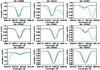 |
Fig. C.2 As Fig. C.1, but for model d8v. |
| In the text | |
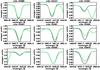 |
Fig. C.3 As Fig. C.1, but for model s10a. |
| In the text | |
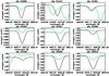 |
Fig. C.4 As Fig. C.1, but for model s8a. |
| In the text | |
|
Fig. C.5 Comparison of N iii line profiles from present work (black) and cmfgen (green), for model d10v. |
| In the text | |
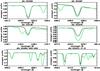 |
Fig. C.6 As Fig. C.5, but for model d8v. |
| In the text | |
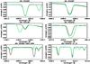 |
Fig. C.7 As Fig. C.5, but for model d6v. |
| In the text | |
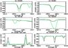 |
Fig. C.8 As Fig. C.5, but for model d4v. |
| In the text | |
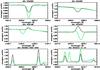 |
Fig. C.9 As Fig. C.5, but for model d2v. |
| In the text | |
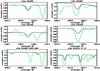 |
Fig. C.10 As Fig. C.5, but for model s10a. |
| In the text | |
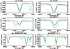 |
Fig. C.11 As Fig. C.5, but for model s8a. |
| In the text | |
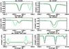 |
Fig. C.12 As Fig. C.5, but for model s6a. |
| In the text | |
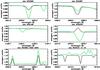 |
Fig. C.13 As Fig. C.5, but for model s4a. |
| In the text | |
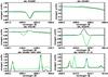 |
Fig. C.14 As Fig. C.5, but for model s2a. |
| In the text | |
Current usage metrics show cumulative count of Article Views (full-text article views including HTML views, PDF and ePub downloads, according to the available data) and Abstracts Views on Vision4Press platform.
Data correspond to usage on the plateform after 2015. The current usage metrics is available 48-96 hours after online publication and is updated daily on week days.
Initial download of the metrics may take a while.