| Issue |
A&A
Volume 536, December 2011
|
|
|---|---|---|
| Article Number | A58 | |
| Number of page(s) | 24 | |
| Section | Stellar atmospheres | |
| DOI | https://doi.org/10.1051/0004-6361/201117101 | |
| Published online | 07 December 2011 | |
Online material
Appendix A: Dielectronic recombination: implementation to fastwind
In the present work we implemented dielectronic recombination into fastwind, which, so far, could not (or only approximately) deal with this process. To this end, new rates (both for the dielectronic recombination and for the inverse process) had to be inserted into the system of the rate equations.
A.1. Explicit method
To calculate these rates for the “explicit method” (see Sect. 3.2), we follow the formulation as provided by Nussbaumer & Storey (1983). In compact notation, the dielectronic recombination for an element X and charge m + 1 proceeds via 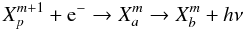 (A.1)where p is a parent state of the m + 1 times ionized element X, a is an autoionizing state and b is a bound state. We denote the initial state of expression A.1, composed of the recombining ion and the free electron, as a continuum state c. We refer to the first process as dielectronic capture and to its inverse as autoionization. In general, dielectronic captures and autoionizations link state a to a large number of continuum states c.
As a final result29, Nussbaumer & Storey (1983) could express the dielectronic recombination coefficient between autoionizing state a and bound state j, αDR(aj), as 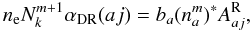 (A.2)with
  the corresponding radiative transition probability for the stabilizing transition (Einstein coefficient for spontaneous emission, corrections for induced emission will be applied below), total ion density
  (element k),
  the LTE population of state a with respect to the actual (NLTE) ground-state population of the next higher ion and the actual electron density, and ba the related NLTE departure coefficient.
The last quantity can be expressed in terms of (i) the autoionization coefficient(s),  , between state a and all possible compound-states c that can form a, (ii) the radiative transition probabilities,
  , between state a and all possible bound and autoionizing states with lower energy i to which state a can decay, and (iii) the departure coefficients of the contributing parent levels, bp (here with respect to the ground-state of the same ion,
  )
) 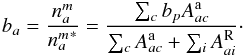 (A.3)Usually, the autoionizing probabilities for state a are much larger than the radiative probabilities for decay, and often there is only one parent level, namely the ground-state of ion m + 1,
  , i.e., bp = 1. Under these conditions (which are similar for excited parent levels assumed to be in LTE with respect to the ground level), ba → 1, and the dielectronic rate depends only on the LTE population of state a and the radiative transition probability . All dependencies on the autoionization probabilities have “vanished”, and we need only the value of that can be derived from the Saha-equation and the ground-state population of ion m + 1, without including the autoionizing levels into the rate equations.
In stellar atmospheres, one needs (in addition to the spontaneous emission to level j) to account for stimulated emission as well, i.e., 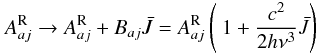 (A.4)with Baj the Einstein coefficient for stimulated emission and
  the scattering integral (profile weighted, frequency integrated mean intensity) for the stabilizing transition. Since the important resonances are broad, the scattering integrals might be replaced by the mean intensities, Jν, of the pseudo-continuum (i.e., including all background opacities/emissivities) at the frequency of the stabilizing line.
Finally, we can define the total dielectronic rate to level j from any possible autoionizing state ai, 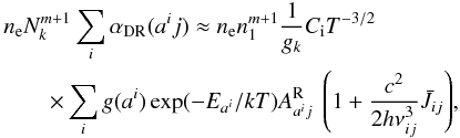 (A.5)which might need to be augmented by departure coefficients bai inside the rhs sum if the parent levels are not the ground-state or not in LTE with respect to the ground-state. The inverse upward rate involves only the line process(es),
 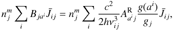 (A.6)with Bji the Einstein-coefficient(s) for absorption. It is easy to show that for LTE conditions (
 and Planckian radiation in the lines) the upward and downward rates cancel each other exactly, as required for thermalization.
Though we have followed here the derivation by Nussbaumer & Storey (1983), our final results for the downward and upward rates are identical with the formulation as used by Mihalas & Hummer (1973) in their investigation.
These rates have been implemented into fastwind and are used whenever the “explicit method” is applied. The only input parameters that need to be specified in the atomic data input file are the transition frequencies and the oscillator-strengths for the stabilizing lines, fja, which relate to the products  via
via 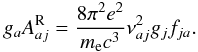 (A.7)For convenience and for consistency with the formulation of “normal” recombination rates (see Sect. A.2), the quantity is expressed in terms of the LTE-population (with respect to actual ionization conditions) of the lower, stabilizing level
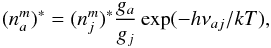 (A.8)so that the downward rate (for a specific autoionizing level a) can be expressed as
 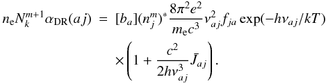 (A.9)Summation over all contributing autoionizing states yields the final rate.
In this explicit method, the rates for dielectronic recombinations and inverse processes are calculated in a separate step and then added to the rates involving resonance-free photoionization cross-sections alone. In our model ion (Sect. 4), we use such cross-sections defined in terms of the Seaton approximation (Eq. (4)), which, together with the data for the stabilizing transitions, have been taken from the wm-basic atomic database. Note that we consider processes both from/to ground-states as well as from/to excited states within ion m + 1, so far on the assumption that the autoionizing levels are in LTE (i.e., without including these levels into the model atom and rate equations).
A.2. Implicit method
Within the implicit method, the DR contribution is already contained within the “conventional” recombination rates, (nj/nk)∗Rkj, to yield a total number of recombinations 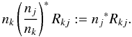 (A.10)As usual, nk is the actual population of the recombining ion in state k and (nj/nk) ∗ the LTE population ratio of the considered level to which the process recombines (either directly or via the intermediate doubly excited state). Rkj is defined as
 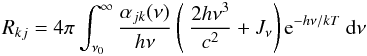 (A.11)with mean intensity Jν and total photoionization cross-section (including resonances), αjk(ν).
In the following, we show that this formulation is consistent with the rates derived in Sect. A.1. We split the cross-section into a resonance-free contribution, and a contribution from the resonances, 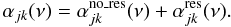 (A.12)The total recombination rate is then the sum of direct and dielectronic recombination,
 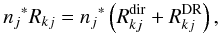 (A.13)with
 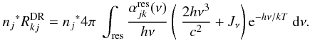 (A.14)The resonances are narrow enough so that most of the frequency dependent quantities can be drawn in front of the integral, evaluated at the average position of the resonances i,
 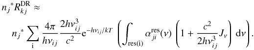 (A.15)The integral over the cross-sections of the resonances corresponds to the cross-section of the stabilizing transitions,
 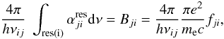 (A.16)with Einstein-coefficient Bji and oscillator-strength fji. Likewise,
 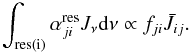 Then, indeed, we recover the result from Eq. (A.9) (explicit formulation),
 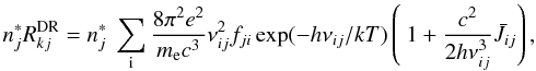 (A.17)if, as outlined in Sect. A.1, the autoionizing levels are in or close to LTE. Note that this is a necessary condition for the implicit method to yield reliable results30, otherwise one has to use exclusively the explicit approach and to include the autoionizing levels into the model atom and rate equations.
The proof that the rates for the inverse photoionization process, calculated either by the implicit method (using total photoionization cross-sections) or via rates from resonance-free cross-sections plus rates involving the excitation of the second electron, are consistent, is analogous and omitted here.
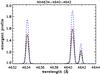 |
Fig. A.1
Consistency of implicit and explicit method. Comparison of N iiiλλ4634 − 4640 − 4642 profiles from model “T3740”, for calculations using a different treatment of DR to the 3d level. Implicit method (solid/black), explicit method (dotted/red), explicit method with oscillator strength for the stabilizing transition increased (dashed/blue) and decreased (dashed-dotted/black) by a factor of two. |
| Open with DEXTER | |
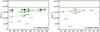 |
Fig. B.1
Grotrian diagrams for the N iii doublet (left) and quartet (right) system. Level numbers refer to Table B.1. Levels # 8, 10, 11 refer to the 3s, 3p and 3d levels involved in the formation of N iiiλλ4634 − 4640 − 4642, and # 3, 4, 5 refer to levels 2p2 (2D, 2S, 2P) that drain level 3p via “two electron transitions”. Important optical transitions are indicated by green lines and numbers referring to Table 4 in the main section. |
| Open with DEXTER | |
A.3. Consistency check
To check the consistency of our implementation of implicit and explicit DR treatment, we carried out the following test. First, to ensure consistent data, we derived the oscillator strength corresponding to the wide PEC resonance in the total photoionization cross-section (Fig. 2) by integrating over the cross-section and applying Eq. (A.16)31. The resulting value (f = 0.45, which is somewhat smaller than the data provided by the wm-basic database, f = 0.60) was then used within the explicit method, at the original wavelength (which coincides with the position of the resonance). As displayed in Fig. A.1 for the case of model “T3740” with “pseudo line-blanketing” (see Sect. 5.1), both methods result in very similar line profiles for the N iii emission triplet, proving their consistency. Figure A.1 also displays the strong reaction of the N iii triplet when the oscillator strength is either increased or diminished by a factor of two.
Appendix B: Details on the N iii model ion
Table B.1 displays the electronic configurations and term designations of our N iii ionic model, and Fig. B.1 the corresponding Grotrian diagrams for the doublet and the quartet systems, indicating important diagnostic transitions in the optical (cf. Sect. 6).
Appendix C: Comparison of line profiles with results from cmfgen
In this appendix, we display a comparison of N iii (and partly N ii) line profiles from fastwind (black) and cmfgen (green), for all models from the grid presented in Table 3. For a discussion, see Sect. 6.
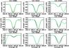 |
Fig. C.1
Comparison of N ii line profiles from present work (black) and cmfgen (green), for model d10v (for parameters, see Table 3). |
| Open with DEXTER | |
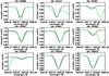 |
Fig. C.2
As Fig. C.1, but for model d8v. |
| Open with DEXTER | |
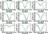 |
Fig. C.3
As Fig. C.1, but for model s10a. |
| Open with DEXTER | |
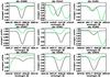 |
Fig. C.4
As Fig. C.1, but for model s8a. |
| Open with DEXTER | |
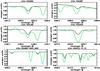 |
Fig. C.5
Comparison of N iii line profiles from present work (black) and cmfgen (green), for model d10v. |
| Open with DEXTER | |
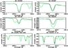 |
Fig. C.6
As Fig. C.5, but for model d8v. |
| Open with DEXTER | |
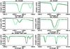 |
Fig. C.7
As Fig. C.5, but for model d6v. |
| Open with DEXTER | |
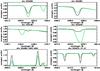 |
Fig. C.8
As Fig. C.5, but for model d4v. |
| Open with DEXTER | |
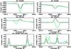 |
Fig. C.9
As Fig. C.5, but for model d2v. |
| Open with DEXTER | |
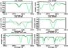 |
Fig. C.10
As Fig. C.5, but for model s10a. |
| Open with DEXTER | |
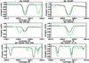 |
Fig. C.11
As Fig. C.5, but for model s8a. |
| Open with DEXTER | |
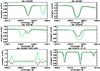 |
Fig. C.12
As Fig. C.5, but for model s6a. |
| Open with DEXTER | |
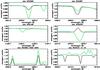 |
Fig. C.13
As Fig. C.5, but for model s4a. |
| Open with DEXTER | |
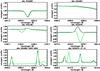 |
Fig. C.14
As Fig. C.5, but for model s2a. |
| Open with DEXTER | |
© ESO, 2011
Current usage metrics show cumulative count of Article Views (full-text article views including HTML views, PDF and ePub downloads, according to the available data) and Abstracts Views on Vision4Press platform.
Data correspond to usage on the plateform after 2015. The current usage metrics is available 48-96 hours after online publication and is updated daily on week days.
Initial download of the metrics may take a while.