| Issue |
A&A
Volume 536, December 2011
|
|
|---|---|---|
| Article Number | A99 | |
| Number of page(s) | 14 | |
| Section | Interstellar and circumstellar matter | |
| DOI | https://doi.org/10.1051/0004-6361/201116438 | |
| Published online | 15 December 2011 | |
Distances to dense cores that contain very low luminosity objects
1 Aryabhatta Research Institute of Observational Sciences, Manora Peak, Nainital 263 129, India
e-mail: This email address is being protected from spambots. You need JavaScript enabled to view it.
2 Korea Astronomy & Space Science Institute, 61-1 Hwaam-dong, Yusung-gu, Daejeon 305-348, Korea
e-mail: This email address is being protected from spambots. You need JavaScript enabled to view it.
3 Astrophysics Group, Blackett Laboratory, Imperial College London, SW7 2AZ, UK
e-mail: This email address is being protected from spambots. You need JavaScript enabled to view it.
Received: 5 January 2011
Accepted: 3 October 2011
Abstract
Aims. We estimate the distances to dense molecular cores that harbour very low luminosity objects (VeLLOs) detected by the Spitzer Space Telescope and attempt to confirm their VeLLO nature.
Methods. The cloud distances are estimated using a near-IR photometric method. We use a technique that performs a spectral classification of stars lying towards the fields containing the clouds as either main-sequence stars or giants. In this technique, the observed (J − H) and (H − Ks) colours are dereddened simultaneously using trial values of AV and a normal interstellar extinction law. The best fit of the dereddened colours to the intrinsic colours giving a minimum value of χ2 then yields the corresponding spectral type and AV for the star. The main-sequence stars, thus classified, are then utilized in an AV versus distance plot to bracket the cloud distances. The typical error in the estimation of distances to the clouds are found to be ~18%.
Results. We estimate distances to seven cloud cores, IRAM 04191, L1521F, BHR 111, L328, L673-7, L1014, and L1148 using the above method. These clouds contain VeLLO candidates. The estimated distances to the cores are found to be 127 ± 25 pc (IRAM 04191), 136 ± 36 pc (L1521F), 355 ± 65 pc (BHR 111), 217 ± 30 pc (L328), 240 ± 45 pc (L673-7), 258 ± 50 pc (L1014), and 301 ± 55 pc (L1148). We re-evaluated the internal luminosities of the VeLLOs discovered in these seven clouds using the distances estimated from this work. Except for L1014 − IRS (Lint = 0.15 L⊙), all other VeLLO candidates are found to be consistent with the definition of a VeLLO (Lint ≤ 0.1 L⊙). In addition to the cores that harbour VeLLO candidates, we also obtained distances to the clouds L323, L675, L676, CB 188, L1122, L1152, L1155, L1157, and L1158, which are located in the directions of the above seven cores. Towards L1521F and L1148, we found evidence of multiple dust layers.
Key words: ISM: clouds / methods: statistical / stars: formation / dust, extinction / stars: low-mass / stars: distances
© ESO, 2011
1. Introduction
Some of the important physical parameters required to elucidate the still mysterious processes involved in the formation and evolution of both molecular clouds and pre-main sequence (PMS) stars depend crucially on the accurate determination of their distances. However, distances to most star-forming and starless molecular clouds, especially those that are relatively isolated, are highly uncertain (Hilton & Lahulla 1995). Furthermore, the need to determine accurate distances to cloud cores can be understood from the discoveries of embedded sources with luminosities less than 0.1 L⊙, called very low luminous objects (VeLLOs), in a number of dense cores that were previously considered as starless (Young et al. 2004; Kauffmann et al. 2005; Dunham et al. 2006; Bourke et al. 2006; Lee et al. 2009; Dunham et al. 2010a). Since the luminosity depends on distance squared, small errors in distance are effectively doubled. Therefore, the above conclusions on the status of these objects as VeLLOs depend crucially on the distances to the parent clouds, which are highly uncertain (in some cases by over a factor of 2). For example, the authors who carried out studies on the VeLLO in L1014 have assumed a distance of 200 pc to the cloud . In contrast, Morita et al. (2006) quoted a distance of 400–900 pc to L1014, which would imply that its resident VeLLO, with a luminosity of L ~ 0.09 L⊙ (calculated using the assumed distance of 200 pc to the cloud) becomes 0.36 − 1.8 L⊙ and ceases to be a VeLLO.
Dense cores were previously considered to be starless if they do not contain an Infrared Astronomical Satellite (IRAS) point source to a sensitivity of L ~ 0.1 L⊙(d/140)2. However, Spitzer observations of L1014, which is considered as a starless core, as a part of Spitzer Legacy program “From Molecular Cores to Planet Forming Disks” (or c2d; Evans et al. 2003) came as a surprise! The core L1014 was found to contain an embedded source, L1014 − IRS, with a very low luminosity of L ~ 0.09 L⊙(Young et al. 2004; Bourke et al. 2005; Huard et al. 2006). The VeLLOs in fourteen more cores were identified in the full c2d sample (Dunham et al. 2008). Of these, five of them (including L1014 − IRS) have been studied in detail so far: IRAM 04191 + 1522 (Dunham et al. 2006), L1521F − IRS (Bourke et al. 2006; Terebey et al. 2009), L328 − IRS (Lee et al. 2009), L673-7−IRS (Dunham et al. 2010a) and L1014 − IRS (Young et al. 2004; Bourke et al. 2006; Huard et al. 2006). Sources with such low luminosities are hard to explain on the basis of the standard model of Shu et al. (1987) as the observed luminosities are found to be more than an order of magnitude lower than expected from the model assuming a spherical mass accretion onto a protostellar object located on the stellar/substellar boundary (Dunham et al. 2006). Thus, the discoveries of VeLLOs in dense cores can pose a formidable challenge to our understanding of star formation. Dunham et al. (2010b) showed that the luminosity problem can be resolved and bring the model predictions into closer agreement with the observations if the episodic mass accretion based on the simulation by Vorobyov & Basu (2006) is included in the evolutionary models of Young & Evans (2005). The sources with the lowest luminosities are then those that are observed in quiescent accretion states.
A number of methods have been applied by various authors in the past to determine distances to clouds that are either associated with large complexes or are relatively isolated (e.g., Greenstein & Shapley 1937; McCuskey 1939; Racine 1968; Gottlieb & Upson 1969; Bok & McCarthy 1974; Mattila 1979; Tomita et al. 1979; Snell 1981; Reipurth & Gee 1986; Cernis 1990; Cernis & Straižys 1992; Straižys et al. 1992; Hilton & Lahulla 1993; Kun & Prusti 1993; Kenyon et al. 1994; Bourke et al. 1995a,b; Corradi et al. 1997; Knude & Høg 1998; Peterson & Clemens 1998; Nielsen et al. 2000; Franco 2002; Maheswar et al. 2004; Alves & Franco 2007; Loinard et al. 2007; Maheswar et al. 2010; Dzib et al. 2010; Knude 2010; Knude & Kaltcheva 2010). Among the methods, the trigonometric parallaxes measured using multi-epoch very long baseline array observations of radio-emitting young stars associated with the clouds can provide distances to the corresponding clouds with a precision of about 1–4% (Loinard et al. 2007, 2008; Torres et al. 2009). However, this method can be applied only to clouds that harbour radio-emitting young stars. Most of the other aforementioned methods are in general extremely tedious and demanding in terms of telescope time. Maheswar et al. (2004) in an earlier study utilized optical and Two Micron all Sky Survey (2MASS) data to determine the distance to the cometary globule, CG12. One can combine the optical data from the Naval Observatory Merged Astrometric Dataset (NOMAD) and the 2MASS data in the method given by Maheswar et al. (2004) to estimate distances to molecular clouds. The NOMAD database is basically a merger of data from the Hipparcos (Perryman & ESA 1997), Tycho-2 (Høg et al. 2000), UCAC-2 (Zacharias et al. 2004), and USNO-B1 (Monet et al. 2003) catalogues, supplemented by photometric data from the 2MASS. However the data available in this catalog is heterogeneous as the observations were carried at different epochs and the accuracy of the photometry required by the method is high ( ≤ 0.1 mag) in BVR. Hence, it would be extremely useful to develop a method that utilizes the vast homogeneous JHKs photometric data produced by the 2MASS, which are already available for the entire sky, to determine the distances to the clouds. The near-IR photometric method presented in a previous pilot study (Maheswar et al. 2010) to estimate the cloud distances was such an endeavour. This method gives distances to clouds that are relatively close ( ≲ 500 pc) with a precision of ~20%.
In this paper, we estimate the distances to seven cloud cores namely, IRAM 041911, L1521F, BHR 111, L328, L673-7, L1014, and L1148, which were previously identified to harbour VeLLO candidates (Dunham et al. 2008), using a near-IR photometric method (Maheswar et al. 2010). Of the seven cloud cores, two of them, IRAM 04191 and L1521F are assocated with the Taurus molecular cloud complex for which very accurate distance measurements are available (Loinard et al. 2007; Torres et al. 2007, 2009). We included them to ascertain the reliability of the method. For the remaining five cores, most authors have used distances that were either guessed or assumed. The distance estimates available in the literature for each cloud core, prior to this study, are discussed along with our results in Sect. 3.1. This paper is organized in the following manner. A brief description of the method and the data used to estimate cloud distances is given in Sect. 2. The estimated distances of the clouds are presented in Sect. 3.1. The consequences of the new distance estimates from this work for the status of the VeLLO candidates are discussed in Sect. 3.2. In Sect. 4, we conclude the paper with a summary of our results.
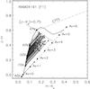 |
Fig. 1 The (J − H) vs. (H − Ks) CC diagram drawn for stars (with AV ≥ 1) from the region F1 towards IRAM 04191 (see Fig. 4) to illustrate the method. The solid curve represents the locations of unreddened main-sequence stars. The reddening vector for an A0V type star drawn parallel to the Rieke & Lebofsky (1985) interstellar reddening vector is shown by the dashed line. The locations of the main-sequence stars of different spectral types are marked with square symbols. The region to the right of the reddening vector is known as the NIR excess region and corresponds to the location of PMS sources. The dash-dot-dash line represents the loci of unreddened CTTSs (Meyer et al. 1997). The line (J − Ks) ≤ 0.75 is the upper limit set to eliminate M-type stars from the analysis as unreddened M-type stars located across the reddening vectors of A0-K7 dwarfs make it difficult to differentiate the reddened A0-K7 dwarfs from the unreddened M-type stars. The circles represent the observed colours and the arrows are drawn from the observed to the final colours obtained by the method for each star. |
The J2000 coordinates of the cores as obtained from SIMBAD.
2. The data and the method
Below we present a brief discussion on the method2. We extracted the J, H, and Ks magnitudes of stars from the 2MASS all-Sky Catalog of Point Sources (Cutri et al. 2003) that satisfied the following criteria of (a) a photometric uncertainty3σ ≤ 0.035 in all the three filters and (b) a photometric quality flag of “AAA” in all the three filters, i.e., signal-to-noise ratio (SNR) > 10. We then selected the stars for which (J − Ks) ≤ 0.75 to eliminate M-type stars from the analysis as unreddened M-type stars located across the reddening vectors of A0-K7 dwarfs make it difficult to differentiate the reddened A0-K7 dwarfs from the unreddened M-type stars. In addition, the classical T Tauri stars (CTTSs), often found to be associated with the molecular clouds, occupy a well-defined locus in the near-infrared colour–colour (NIR-CC) diagram (Meyer et al. 1997) as shown in Fig. 1, which intercepts with the main-sequence loci at (J − Ks) ≈ 0.75. Thus, the criterion of (J − Ks) ≤ 0.75 would also allow us to eliminate most of the CTTSs.
A set of dereddened colours for each star were produced from their observed colours by using a range of trial values of AV (0–10 mag) and the Rieke & Lebofsky (1985) reddening law. The choice of a photometric uncertainty, σ ≤ 0.035, ensures that the stars are selected from relatively low extinction regions of the cloud where the Rieke & Lebofsky (1985) reddening law is most applicable (Straizys et al. 1982; Kandori et al. 2003). The computed sets of dereddened colours of a star were then compared with the intrinsic colours of the normal main-sequence stars. The intrinsic colours of the main-sequence stars in the spectral range A0-K7 were taken from Maheswar et al. (2010). The best match giving a minimum value of χ2 then yielded the spectral type and AV corresponding to that intrinsic colour. Once the spectral types and AV values of the stars were known, their distances were estimated using the distance equation, d (pc) = 10(Ks − MK + 5 − AK)/5. Only those stars that were classified as dwarfs were considered for the determination of distances as the absolute magnitudes of giants are highly uncertain. The whole procedure is illustrated in Fig. 1 where we plot the NIR-CC diagram for stars (with AV ≥ 1) chosen from the region F1 towards the direction of IRAM 04191 (see Fig. 4). The arrows are drawn from the observed data points to the corresponding dereddened colours estimated using the method. The maximum extinction values that can be measured using the method are those for A0V type stars (≈4 mag). The extinction traced by stars decreases as we move towards more late type stars.
To estimate the distance to a cloud (not just by eye estimation), we first grouped the stars, classified as dwarfs, into distance bins of bin width = 0.18 × distance. The centres of each bin were kept at a separation of half the bin width. Since there are very few stars at smaller distances, the mean value of the distances and the AV of the stars in each bin were calculated by taking 1000 pc as the initial point and proceeding towards smaller distances. The mean distance of the stars in the bin at which a significant drop in the mean extinction occurred was taken as the distance to the cloud, and the average uncertainty in the distances of the stars in that bin was taken as the final uncertainty in the determined distance of the cloud (see Figs. 2 and 3). The vertical dashed line in the AV versus (vs.) d plots, used to mark the cloud distance, is drawn at a distance deduced from the above procedure. The error in the mean values of AV were calculated using the expression, ![Mathematical equation: \hbox{$standard~deviation/\sqrt[]{N}$}](/articles/aa/full_html/2011/12/aa16438-11/aa16438-11-eq43.png) , where N is the number of stars in each bin. The AV values were found to be uncertain by ~0.6 mag. The typical errors in our distance estimates for the clouds were found to be ~18% (Maheswar et al. 2010).
, where N is the number of stars in each bin. The AV values were found to be uncertain by ~0.6 mag. The typical errors in our distance estimates for the clouds were found to be ~18% (Maheswar et al. 2010).
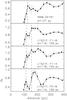 |
Fig. 2 The mean values of AV vs. the mean values of distance plot for IRAM 04191 and L1521F produced using the procedure discussed in Sect. 2 to determine distances to the clouds. The error bars in the mean AV values were calculated using the expression, |
One of the prominent features of the molecular cloud structure is that it is hierarchical. The extinction maps produced towards a number of regions in our Galaxy, using optical and near-infrared techniques, have shown that the high-density features are invariably contained within an extended low-density envelope (e.g., Dobashi et al. 2005; Lombardi et al. 2010). Our method utilizes the background stars shining through the outer low-extinction (AV ≲ 4 mag) regions of the cores to estimate their distances. When there is a single dust layer along the line of sight, we expect a sharp increase in extinction for stars located behind that dust layer in an AV vs. d plot. The distance at which the sharp increase in the extinction occurs is considered as the distance to that dust layer. However, if there is more than one dust layer along the line of sight, we expect a steep but step-like increase in the extinction at distances at which the dust layers are located. This, however, happens only if the foreground dust layers have constant extinction values. In the case of patchy foreground dust layer(s), this method can give distance only to the first layer as the sharp step-like features are smeared by the non-uniform extinction caused by the foreground dust layer.
Knude (2010), using the 2MASS data, presented a similar method to estimate distances to molecular clouds. Instead of using the main-sequence stars in the spectral range from A0-K7 as in our work, Knude (2010) utilized three spectral groups. Of O-G6 as primary sources, M4-T as secondary sources, and G6-M0 as teritary sources in the estimation of the cloud distances. The absolute magnitude in J-band was calibrated using Hipparcos stars. Following a rigorous statistical approach, the jump in the extinction in the AV vs. distance plot was obtained to determine the distance. In thus pilot study, Knude (2010) estimated distances to a number of nearby clouds including Chamaeleon I and Lupus 3, which were also studied in Maheswar et al. (2010). The distance estimates in both of these works are found to be in good agreement within the errors (the typical error in the distance estimates of Knude (2010) was found to be ~8%).
The details of the fields selected towards each cloud.
3. Results and discussion
3.1. Distances to the cloud cores IRAM 04191, L1521F, BHR 111, L328, L673-7, L1014, and L1148
We applied the method to seven dense cores, namely IRAM 04191, L1521F, BHR 111, L328, L673-7, L1014, and L1148. We divided the fields containing the cores into small sub-fields to avoid complications created by the erroneous classifications of giants into dwarfs. While the rise in the extinction caused by a cloud should occur almost at the same distance in all the fields, if the whole cloud were located at the same distance, the wrongly classified stars in the sub-fields would show high extinction not at the same but at random distances (Maheswar et al. 2010). For cores with small angular sizes, we included fields containing additional cores that are located spatially closer and have similar radial velocities (obtained, for example, from CO observations), to have a sufficient number of stars to infer their distances. Here we assume that the cores that are spatially closer and have similar velocities are located at almost the same distances. Table 2 summarizes the area of the fields (in degree) chosen towards the cores studied here, the Galactic coordinates of the centre of the fields, the total number of stars selected after applying all the selection criteria (σ ≤ 0.035, SNR > 10, and (J − Ks) ≤ 0.75) and the number of stars classified as dwarfs by our method towards each field. Below we present our results and discussion of individual clouds. In the AV vs. d plots presented for the studied cores, the dash-dotted curve shows the increase in extinction towards the cloud Galactic latitude as a function of distance produced using the expressions given by Bahcall & Soneira (1980, hereafter BS80). The dashed vertical line(s) is drawn at the cloud distance(s) inferred from the procedure described in Sect. 2 (see Figs. 2 and 3).
3.1.1. IRAM 04191
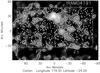 |
Fig. 4 The 2° × 3° extinction map produced by Dobashi et al. (2005) of the region containing IRAM 04191. The contours are drawn at 0.4, 0.6, 0.8, and 1.0 mag levels. The fields used for selecting star to determine distance are identified and labelled. The stars classified as dwarfs and used for determining distance to the cloud are identified using open circles. |
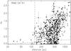 |
Fig. 5 The AV vs. d plot for all the stars classified as dwarfs from the fields F1-2 combined together towards IRAM 04191. The dashed vertical line is drawn at 127 pc inferred from the procedure described in Sect. 2 (see Fig. 3). The dash-dotted curve represents the increase in extinction towards the Galactic latitude of b = −24° as a function of distance produced from the expressions given by BS80. The error bars are shown for a few stars to ensure that the data points can be seen more clearly. |
We show the 3° × 2° extinction map4 produced by Dobashi et al. (2005) of the region containing IRAM 04191 in Fig. 4. The contours are drawn at 0.4, 0.6, 0.8, and 1.0 magnitude levels. We selected two fields, F 1 and F2, each covering an area of 1° × 1° as shown in Fig. 4. The stars, classified as dwarfs, that are used to determine the distance to the cloud are identified using circles.
In Fig. 5, we present the AV vs. d plot for the stars from both F1 (filled circles) and F2 (open circles) combined together. The dashed vertical line is drawn at 127 pc. The jump in the extinction values significantly above the value expected from the expression of BS80 is found to occur, in both fields, at ~127 pc. Beyond this distance, the stars with high extinction are found to be distributed almost continuously in distance as one would expect because the cloud should act as a dense dust layer that dims the stars shining through it. Using 541 stars classified as main-sequence stars, we estimated a distance of 127 ± 25 pc to the cloud IRAM 04191.
Very accurate distance determinations ( ≲ 1%) are available for a number of naked T Tauri stars associated with the Taurus molecular cloud complex from the trigonometric parallax measurements made using the Very Long Baseline Array (VLBA) multi-epoch observations carried out by detecting their non-thermal 3.6 cm radio continuum emission. These stars include, HDE 283572, Hubble 4, T Tau, and HP Tau/G2. They are found to be located at distances of 128.5 ± 0.6 pc (Torres et al. 2007), 132.8 ± 0.5 pc (Torres et al. 2007), 147.6 ± 0.6 pc (Loinard et al. 2007), and 161.2 ± 0.9 pc (Torres et al. 2009), respectively. As of now, from the distances determined for these four stars, it is apparent that the clouds in the Taurus molecular cloud complex are distributed in space at distances ranging from ~128 pc to ~161 pc. From the mean parallax obtained from the above four stars, Torres et al. (2009) determined a mean distance of 141.2 pc to the Taurus cloud complex. At a distance of 127 ± 25 pc, IRAM 04191 could possibly be located at the front end of the Taurus cloud complex. In all previous studies of IRAM 04191, this cloud was considered to be associated with the Taurus cloud complex and assigned a distance of 140 pc (Kenyon et al. 1994). The distance estimate presented here is the first independent confirmation of the association of IRAM 04191 with the Taurus cloud complex.
3.1.2. L1521F
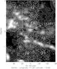 |
Fig. 6 The ~3° × 4° extinction map produced by Dobashi et al. (2005) of the region containing L1521F. The contours are drawn at 0.5, 1.0, 1.5, 2.0, 2.5, and 3.0 mag levels. The fields used to select stars to determine distance are identified and labelled. L1521F is located in F3. |
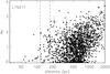 |
Fig. 7 The AV vs. d plot for all the stars classified as dwarfs from the fields F1-8 combined together towards L1521F. The dashed vertical lines are drawn at distances 116 pc and 156 pc inferred from the procedure described in Sect. 2 (see Fig. 3). The dash-dotted curve represents the increase in the extinction towards the Galactic latitude of b = −14.9° as a function of distance produced from the expressions given by BS80. The error bars are shown for only a few stars. |
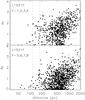 |
Fig. 8 The AV vs. d plot for the stars classified as dwarfs from the fields F1-4 in the upper panel and F5-8 in the lower panel towards L1521F. The dashed vertical lines are drawn at 116 pc and 156 pc. The dash-dotted curve represents the increase in the extinction towards the Galactic latitude of b = −14.9° as a function of distance produced from the expressions given by BS80. The error bars are shown for only a few stars. |
Figure 6 shows the ~3° × 4° extinction map of the region containing L1521F. The contours are drawn at 0.5, 1.0, 1.5, 2.0, 2.5, and 3.0 magnitude levels. We divided the region containing L1521F into eight fields, F1-8, as shown in Fig. 6. Each field covers an area of 1° × 1°. The stars, classified as dwarfs, that are used to determine distances to the cloud are identified using circles. The cloud L1521F is located in the field F3.
In Fig. 7, we present a AV vs. d plot for the stars in all the fields (F1-8) combined together. The dashed vertical lines are drawn at 116 and 156 pc. Though, in Fig. 7, only one component of dust layer is apparent, we can discern two dust layers in Fig. 2 as illustrated by a sharp rise in the mean values of extinction occurring at two distances, one at 116 pc and another at 156 pc. In the AV vs. d plots of individual fields, we found that the dust layer at 116 pc is more conspicuous towards the fields F1-4, than towards the fields F5-8. In Fig. 8, we present the AV vs. d plot for the stars from the fields F1-4 (upper panel) and F5-8 (lower panel) separately to show the dominance of the two components of dust layers in these two regions. In Fig. 2 we show the distances determined using the stars from F1-4 and F5-8 independently. The two dust layers are found to be at distances 118 ± 22 pc and 155 ± 29 pc and then 114 ± 21 pc and 156 ± 29 pc towards the fields F1-4 and F5-8, respectively. The distances estimated for the two dust components using stars from separate sets of fields are found to be in good agreement. These results demonstrate that the technique employed here to estimate the distances to dust layers in a particular direction is capable of selecting them consistently, even though the fields (1° × 1° each) used to select the stars are located relatively far (3°−4° in this case) apart.
The dust layer at ~156 pc seems to be present in all the eight fields. In addition, the AV vs. d plot produced for the sources from F5-8 contain a number of stars that show high extinction at distances smaller than ~156 pc. This might be due to the contribution of the dust component at ~114 pc. One of the limitations of the method is that in case of multiple jumps in extinction in an AV vs. d plot, it is difficult to associate a particular jump with any of the dust layer. This is true for all the methods that utilize the rise in the extinction as a way to estimate distances.
The above findings encouraged us to estimate distances to the entire Taurus molecular cloud complex. We identified four dust components at distances 85 ± 16, 114 ± 20, 138 ± 25, and 168 ± 31 pc in the direction of the cloud. Our results will be presented in a forthcoming paper. The presence of a dust component at ~85 pc, however, is found to be less clearly evident towards the entire cloud complex. Since the dust layer at ~118 pc is found to be the dominant layer towards F3, the field in which L1521F is located, we associate the jump at ~118 ± 22 pc with the cloud L1521F. However adopting a mean value of 136 ± 36 pc (with an error in this case of  ) to L1521F would be more appropriate as it is closer to the distances of two sources, HDE 283572 and Hubble 4, found to be located nearer (<2°) to L1521F and more precisely at distances 128.5 ± 0.6 pc and 132.8 ± 0.5 pc, respectively (Torres et al. 2009).
3.1.3. BHR 111
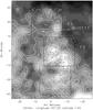 |
Fig. 9 The ~1.5° × 1.5° extinction map produced by Dobashi et al. (2005) of the region containing BHR 111. The contours are drawn at 2, 2.1, 2.2, 2.3, and 2.4 mag levels. The fields used to select stars to determine distance are identified and labelled. The stars classified as dwarfs and used to determine distance to the cloud are identified using open circles. |
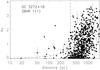 |
Fig. 10 The AV vs. d plot for all the stars classified as dwarfs from the fields F1-3 combined together towards BHR 111. The dashed vertical line is drawn at 355 pc inferred from the procedure described in Sect. 2 (see Fig. 3). The dash-dotted curve represents the increase in the extinction towards the Galactic latitude of b = 1.824° as a function of distance produced from the expressions given by BS80. The error bars are shown for only a few stars. |
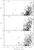 |
Fig. 11 The AV vs. d plot for the stars classified as dwarfs from the individual fields F1, F2, and F3 towards BHR 111. The dashed vertical line is drawn at 355 pc inferred from the procedure described in Sect. 2 (see Fig. 3). The dash-dotted curve represents the increase in the extinction towards the Galactic latitude b = 1.824° as a function of distance based on the expressions given by BS80. The error bars are shown for only a few stars. |
In Fig. 9, we present the ~1.5° × 1.5° extinction map of the region containing BHR 111 (DC 3272+18). The contours are drawn at 2, 2.1, 2.2, 2.3, and 2.4 mag levels. The size of the cloud is only 10′ × 4′(Bourke et al. 1995a). We included two fields F2 and F3 in addition to the field F1, which contains BHR 111, as shown in Fig. 9. Unfortunately, no velocity information is available for the selected regions except for BHR 111 (Bourke et al. 1995a). The stars, classified as dwarfs, that are used to determine the cloud distance are identified using circles.
In Fig. 10, we present the AV vs. d plot of the stars from all the fields (F1-3) combined together. The dashed vertical line is drawn at 355 pc. There are a number of stars that exhibit relatively high extinction values at distances smaller than 355 pc. An inspection of Fig. 11, which presents the AV vs. d plot for stars from the individual fields separately, shows that the jump in the extinction values consistently occurs at or beyond 355 pc. We therefore suspect that there is a foreground dust layer. On the basis of 741 stars classified as dwarfs by the method, we estimate a distance of 355 ± 65 pc to BHR 111.
The distance to BHR 111 was first determined by Bourke et al. (1995b) from a plot of stellar reddening of stars, which had been selected from a circular region centred on the object, against their distances corrected for reddening. They selected stars that had both MK spectral types and colours available. They estimated a distance of 250 pc to BHR 111. Using the same method, Racca et al. (2009) also estimated a distance of 250 pc to BHR 111. Bourke et al. (1995b) used a search radius of 5° about the cloud to find stars with MK spectral types and colours. If an insufficient number of stars were available within 5°, they increased the search radius to either 7.5° or 10°. Racca et al. (2009) used a search radius of 3° about the cloud to select the stars. In Fig. 9, we note that the cloud is not isolated but surrounded by diffuse dust clouds. In Fig. 11, there is evidence of more intervening dust layers towards the line-of-sight that is stronger than towards F3. The large search radius used by both Bourke et al. (1995b) and Racca et al. (2009) might have identified instead a closer dust layer possibly located at 250 pc.
3.1.4. L328
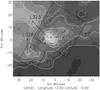 |
Fig. 12 The ~1° × 1° extinction map produced by Dobashi et al. (2005) of the region containing L328. The contours are drawn at 1.5, 2.0, 2.5, 3.0, 3.5, and 4.0 mag levels. The fields used to select stars to determine distances are identified and labelled. The stars classified as dwarfs using the near-IR photometry in each field are shown using filled circles. The fields F1 and F2 cover an area of 0.3° × 0.3° and 0.5° × 0.5°, respectively. |
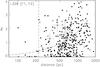 |
Fig. 13 The AV vs. d plot for all the stars classified as dwarfs from the fields F1 (open circles) and F2 (filled circles) combined together towards L328. The dashed vertical line is drawn at 217 pc inferred from the procedure described in Sect. 2 (see Fig. 3). The dash-dotted curve represents the increase in the extinction towards the Galactic latitude of b = −0.829° as a function of distance produced from the expressions given by Bahcall & Soneira (1980). The error bars are shown for only a few stars. |
In Fig. 12 we present the 1° × 1° extinction map of the region containing L328. The contours are drawn at 1.5, 2.0, 2.5, 3.0, 3.5, and 4.0 magnitude levels. We divided the region containing L328 into two fields, F1 and F2, as shown in Fig. 12. The angular extent of L328 (~1′) is found to be too small to divide the field containing the cloud further into smaller sub-fields containing a sufficient number of stars for the analysis. We therefore included the field containing an another molecular core, L323, located in the close vicinity (~20′) of L328. Both the cores, L328 and L323, are found to have similar radial velocities of 6.6 and 6.4 km s-1, respectively (Clemens & Barvainis 1988). The locations of the cores and the fields chosen are identified and labelled in Fig. 12. The stars, classified as dwarfs, that are used to estimate the core distance are identified using circles.
In Fig. 13, we show the AV vs. d plot for the stars in all the fields (F1-2) combined together. The stars from F1 and F2 are represented using open and filled circles, respectively. The field containing L328 is small relative to F2 because of the small angular extent of the cloud. The stars displaying high extinction at/or beyond 217 pc are present in both the fields. There are two stars with AV ≥ 1 mag at distances smaller than 217 pc. Both stars are found to be located towards F2 and to be at different distances. On the basis of 347 sources classified as main-sequence stars from the two fields, we estimated a distance of 217 ± 30 pc to both L328 and L323.
Earlier estimates of distances to L323 (and L328) made by Bok & McCarthy (1974), assumed a distance of 200 pc based on the number of stars brighter than mpg = 21 mag projected onto the cloud in their photographic plate. Later, several authors assigned a distance of 200 pc assuming that the clouds, L328 and L323, are located in-between the Ophiuchus cloud and the Aquila Rift (e.g., Lee et al. 2009). Using photometry on the Vilnius system, Straižys et al. (2003) estimated a distance of 225 ± 55 pc to the front edge of the Aquila Rift with a possible depth of 80 pc to the cloud complex. If L328 and L323 are physically associated with the Aquila Rift, then the clouds are possibly located towards its front edge.
3.1.5. L673-7
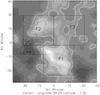 |
Fig. 14 The 1.5° × 1.5° extinction map produced by Dobashi et al. (2005) of the region containing L673-7. The contours are drawn at the 4.0 and 5.0 mag levels. The fields used to select stars to determine distances are identified and labelled. The stars classified as dwarfs using the near-IR photometry in each field are shown using filled circles. Each field covers an area of 0.5° × 0.5°. |
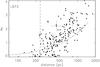 |
Fig. 15 The AV vs. d plot for all the stars classified as dwarfs from the fields F1, F2 and F3 combined together towards L673. The dashed vertical line is drawn at 240 pc inferred from the procedure described in Sect. 2 (see Fig. 3). The dash-dotted curve represents the increase in extinction towards the Galactic latitude b = −1.33° as a function of distance based on the expressions given by BS80. The error bars are shown for only a few stars. |
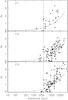 |
Fig. 16 The AV vs. d plot for the stars classified as dwarfs from the individual fields F1 (upper), F2 (middle), and F3 (lower panel) towards L673. The dashed vertical line is drawn at 240 pc inferred from the procedure described in Sect. 2 (see Fig. 3). The dash-dotted curve represents the increase in extinction towards the Galactic latitude b = −1.33° as a function of distance based on the expressions given by BS80. The error bars are shown for only a few stars. |
In Fig. 14, we present the 1.5° × 1.5° extinction map towards the direction of L673-7. The contours are drawn at 4.0 and 5.0 mag levels. We divided the region containing L673-7 into three fields F1, F2, and F3, as shown in Fig. 14. The cloud L673-7 is part of the L673 cloud complex from the Lynds (1962) catalog. Lee & Myers (1999) identified 11 cores within the L673 complex including L673-7. The radial velocity of the complex based on CO line observations is in the range 6.71–7.30 km s-1(Kislyakov & Gordon 1983). Some more clouds are found to be associated with the region selected around L673 namely, L675, L676 from the Lynds (1962) catalog, and CB188 from Clemens & Barvainis (1988). These three clouds also have similar radial velocities of 7.5, 7.6, and 7.1 km s-1, respectively (Clemens & Barvainis 1988), to that of the L673 complex. We therefore assume that the regions selected around L673 are all associated and included in our analysis. The stars, which have been classified as dwarfs, used to determine the cloud distance are identified using circles.
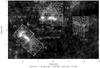 |
Fig. 17 The 2° × 2° extinction map produced by Dobashi et al. (2005) of the region containing LDN 1148. The contours are drawn at 0.7, 1.0, and 2.0 mag levels. The fields used to select stars to determine distances are identified and labelled. Each field is of 0.7° × 0.7°. |
In Fig. 15, we present the AV vs. d plot for the stars from all fields (F1-3) combined together. A jump in the extinction values significantly above the values expected from the expression of BS80 is evident at/or beyond ~240 pc. The stars with high extinction are distributed almost uniformly beyond ~240 pc. In Fig. 16, we show the AV vs. d plot for the stars from the individual fields F1, F2, and F3. In all three fields, the jump in the extinction appears to occur at ~240 pc. Using 199 sources classified as main-sequence stars from the three fields, we estimated a distance of 240 ± 45 pc to L673-7.
Previous estimates of the distance to L673-7 were highly uncertain. Herbig & Jones (1983) used a distance of 300 pc, based on proper motion studies. Others assumed a distance of either 200 pc or 300 pc in their studies (e.g., Hilton & Lahulla 1995; Dunham et al. 2010a). Edwards & Snell (1982) used a distance of 150 pc based on the assumption that L673 is a part of Gould’s belt and characterized it as the minimum distance to the cloud. Since L673, L675, L676, and CB188 have similar radial velocities, we assign a distance of 240 ± 45 pc to all these clouds.
3.1.6. L1148
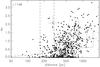 |
Fig. 18 The AV vs. d plot for all the stars classified as dwarfs from the fields F1, F2, F3, and F4 combined together towards L1148. The dashed vertical lines are drawn at 168 pc and 301 pc inferred from the procedure described in Sect. 2 (see Fig. 3). The dash-dotted curve represents the increase in the extinction towards the Galactic latitude b = + 15.3° as a function of distance based on the expressions given by BS80. The error bars are shown for only a few stars. |
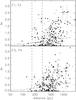 |
Fig. 19 The AV vs. d plot for the stars classified as dwarfs from the individual fields F1 (open circles) and F2 (filled circles) in upper panel and F3 (filled circles) and F4 (open circles) in lower panel towards L1148. The dashed vertical lines are drawn at 168 pc and 301 pc inferred from the procedure described in Sect. 2 (see Fig. 3). The dash-dotted curve represents the increase in extinction towards the Galactic latitude b = + 15.3° as a function of distance based on the expressions given by BS80. The error bars are shown for only a few stars. |
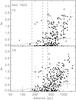 |
Fig. 20 The AV vs. d plot for the stars classified as dwarfs from the individual fields F5 (upper panel) and F6 (lower panel) towards NGC 7023. The dashed vertical lines are drawn at 168 pc, 310 pc, and 408 pc inferred from the procedure described in Sect. 2 (see Fig. 3). The dash-dotted curve represents the increase in extinction towards the Galactic latitude b = + 14.1° as a function of distance based on the expressions given by BS80. The error bars are shown for only a few stars to ensure that the points can be seen more clearly. |
The fields used to determine the distance to L1148 are shown in the extinction map in Fig. 17. The contours are drawn at 0.7, 1.0, and 2.0 mag levels. We divided the region containing L1147/48 into four fields, F1, F2, F3, and F4, as identified in Fig. 17. The stars, classified as dwarfs, that were used to determine the cloud distance are identified using circles.
In Fig. 18, we present the AV vs. d plot for the stars from all the fields (F1-4) combined together. A jump in the extinction values significantly above the values expected from the expression of BS80 is evident at 168 pc. However if we compare the AV vs. d plots of IRAM 04191 and L1521F, which are both located within a 200 pc distance, with that of L1148, we note that the stars with high extinction towards L1148 are not distributed continuously beyond 168 pc. The angular size of the cloud (inferred from the extinction map shown in Fig. 17) is large enough for there to have been a continuous distribution of stars with high extinction beyond 168 pc if the cloud were located at this distance. The lack of such an effect is clearly seen in Fig. 19 where we show the AV vs. d plot for the stars from the individual fields F1 (open circles) and F2 (filled circles) in the upper panel and F3 (filled circles) and F4 (open circles) in the lower panel. Only a few stars are seen with high extinction especially towards the fields F3 and F4. In contrast, a wall of high extinction stars are seen beyond ~300 pc towards all the four fields. Using the stars from F3 and F4 alone, we estimated a distance of 301 ± 55 pc to this dust component.
The L1148 core is located in a cloud complex towards the direction of Cepheus. The most widely quoted distance to L1147/48/55 is 325 ± 13 pc (Straižys et al. 1992). They used the Vilnius photometric system to classify the stars and derived the interstellar reddening. They obtained a distance of 325 ± 13 pc to L1147/1158 by taking an average of the distances to ten stars showing AV ≥ 0.45 that were distributed in the range 240–380 pc. Snell (1981) obtained a distance of 250 pc to L1147 based on the AV vs. d plot produced using the stars from a region of 20° × 20° centred on the cloud that had both optical photometry and MK spectral classification. Kun (1998) found that there are three dust components at characteristic distances of 200, 300, and 450 pc, based on a cumulative distribution of field star distance moduli in Wolf diagrams. A complex velocity structure was reported by Harjunpää et al. (1991) towards the directions of the L1147/48, L1152, L1157, and L1155/58 cloud complexes. They identified two distinct velocity components in 13CO and C18O line profiles. The blueshifted component (VLSR ≈ 1.5 km s-1) was found to have a smaller extent than the redshifted component (VLSR ≈ 2 − 4 km s-1), which was found to be extended over the whole cloud area. On the basis of the velocity structure found over the whole cloud, they discovered two cloud components along the line of sight.
The radial velocities measured for the cores L1148, L1155C-1, and L1155C-2 of the cloud complex are found to be 2.56, 2.58, and 1.35 km s-1, respectively (Lee et al. 2004). Another cloud L1167/1174, which also has a similar radial velocity of 2.67 km s-1(Caselli et al. 2002; Yonekura et al. 1997) similar to that of L1147/48 is found to be located at ~2° south-east of L1147/48/55 cloud complex (see Fig. 17). Straižys et al. (1992) estimated a distance of 288 ± 25 pc to the L1167/1174 again by taking an average distance of four considerably reddened stars. They proposed a distance of 275 pc to HD 200775, which is a Herbig Be star (The et al. 1994) found to be associated with NGC 7023 and responsible for the reflection nebulosity, by assuming that it is a B3Ve star. Maheswar et al. (2010), using the same method employed in this work, estimated a distance of 408 ± 76 pc to NGC 7023, which is consistent with the Hipparcos parallax distance of  pc to HD 200775 (van den Ancker et al. 1998; Bertout et al. 1999). In the direction of NGC 7023, they also found evidence of two additional dust components one at ~ 200 pc and another at 305 pc, distances that are in good agreement with those inferred by Kun (1998). In Fig. 20, we show the AV vs. d plot for the stars from the fields F5 and F6, which contain L1167/1174 complex (see Fig. 17). Step-like features at 310 and 408 pc are clearly visible in the plots. The component at 408 pc seems to be more conspicuous towards F5, where L1174 cloud is located. A continuous distribution of stars with high extinction is apparent beyond 408 pc. The star HD 200775 is probably associated with this cloud component. Towards F6, the dust component found at 310 pc seems to be the most dominant one. There are a number of stars both towards F5 and F6 that show high extinction even at distances smaller that 310 pc, which may be due to a third dust layer along the line of sight.
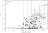 |
Fig. 21 The AV vs. d plot for all the stars classified as dwarfs towards L1122. The dashed vertical lines are drawn at 220 pc, 301 pc, and 408 pc. The dash-dotted curve represents the increase in extinction towards the Galactic latitude b = + 14.8° as a function of distance based on the expressions given by BS80. The error bars are shown for only a few stars to be able to distinguish more clearly between the points. |
About 2° south-west of the L1147/48 cloud complex, there is one more Lynds cloud, L1122, which has a radial velocity of 4.8 km s-1(Yonekura et al. 1997). No earlier distance estimates are available for the cloud. We estimated the distance to this cloud by selecting stars from a region of 1° × 1° (see Fig. 17) centred on the cloud. In Fig. 21, we show the AV vs. d plot for the stars towards L1122. A sudden jump in the extinction is visible at 220 pc. We assigned the distance of the first star that showed AV > 1 as the distance to this cloud. We note that the dust components seen at 310 pc and 408 pc towards L1167/1174 are absent towards L1122. The location of this cloud at a smaller distance proves that there are dust components as close as 200 pc or even less as we found towards L1148. We therefore believe that the dust component seen towards the L1147/48 cloud complex is a foreground layer and that the actual layer is associated with the dust component inferred at 301 pc.
3.1.7. L1014
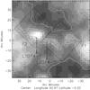 |
Fig. 22 The 1.2° × 1.2° extinction map produced by Dobashi et al. (2005) of the region containing L1014. The contours are drawn at 1.0, 1.5, and 2.0 mag levels. The fields used to select stars to determine distances are identified and labelled. The stars classified as dwarfs using the near-IR photometry in each field are shown using filled circles. Each field is of 0.4° × 0.4°. |
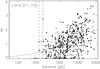 |
Fig. 23 The AV vs. d plot for all the stars classified as dwarfs from the fields F1 and F2 combined together towards L1014. The dashed vertical lines are drawn at 221 pc and 258 pc inferred from the procedure described in Sect. 2 (see Fig. 3). The dash-dotted curve represents the increase in extinction towards the Galactic latitude b = −0.251° as a function of distance based on the expressions given by BS80. The error bars are shown for only a few stars to ensure more clarity in the presentation of the points. |
In Fig. 22, we identify the fields used to select stars in the 1.2° × 1.2° extinction map of L1014. The contours are drawn at the 1.0, 1.5, and 2.0 mag levels. The stars, classified as dwarfs, that are used to determine the cloud distance are identified using circles. Each field covers an area of 0.4° × 0.4°. The angular extent of L1014-2, which contains the VeLLO L1014 − IRS, is only ≈ 2′. Therefore, we included another cloud L1014-1, which is located ~10′ north-east of L1014-2. The cloud L1014-1 is better known as B362. Both L1014-1 and L1014-2 are found to have similar radial velocities (4.0 and 4.2 km s-1 respectively, Lee et al. 1999; Crapsi et al. 2005).
In Fig. 23, we present the AV vs. d plot for the stars from all the fields F1 (filled circles) and F2 (open circles) combined together. In Fig. 3, steep rise in the mean values of extinction are found to occur at distances of 221 pc and 258 pc. However from Fig. 23 it is evident that the steep rise in the extinction at 221 pc occurs mainly because of two stars that are located in the field, F2 alone. In contrast, the steep rise in the mean value of extinction at 258 pc (see Fig. 23) is caused by the stars from both fields, F1 and F2 (filled and open circles). Therefore, we associate the jump in the extinction at 258 pc to the presence of the cores L1014-1/2. In addition, beyond this distance the high extinction stars are distributed almost regularly. However, we found only two stars with low extinction values in the foreground of L1014-1/2; such instances of stars are essential to have a complete census of the dust layers in the direction. To include more cores in the vicinity of L1014-1/2 with similar radial velocities, we examined the large-scale maps of the clouds produced by Dobashi et al. (1994) based on a 13CO (with a 2.7′ angular resolution) survey towards the Cygnus region. The cloud L1014-1, was detected in their survey, and found to be isolated with no cloud components, at least, within a radius of 2° in the velocity range of 3 < VLSR < 4.5 km s-1 (see Fig. 5i of their publication).
Dame & Thaddeus (1985) assigned a distance of 800 pc to L1014 assuming that it is part of Cyg OB7 (see Dobashi et al. 1994). Ho et al. (1978) adopted a distance of 200 pc for B362. Morita et al. (2006) assigned a distance of 400–900 pc to L1014 by assuming that this cloud is associated with identified T Tauri stars with the cloud. No reliable estimate of distance to L1014-2 is available in the literature. In most of the studies carried out on L1014-2, the authors adopted a distance of 200 pc (e.g., Lee & Myers 1999) by assuming that both B362 and L1014-2 are located at same distance. Using a total of 400 sources classified as main-sequence stars from the two fields, we estimated a distance of 258 ± 50 pc to L1014.
3.2. Are VeLLOs really VeLLOs?
On the status of the VeLLOs.
Using the distances estimated to the seven cores in this work, we re-evaluate the internal luminosities of the VeLLO candidates. In Table 3, we list the distances used in earlier studies and the internal luminosities calculated using those distances of the VeLLOs in Cols. 2 and 3, respectively. The re-evaluated internal luminosities of the VeLLOs are given in Col. 6 of Table 3. The previously determined internal luminosities of the VeLLOs in the cores L328, L673-7, and L1014 were calculated using distances that are highly uncertain. However, we find that these distances are very close to the values we have determined in this work. As we can see from Table 3, the re-estimation of the internal luminosities of six VeLLO candidates with our reliable distance measurements confirm them to be consistent with the definition of VeLLOs. The VeLLO associated with L1014-2 core is found to be Lint = 0.15 L⊙. However, this source remains interesting and could be called a VeLLO-like because the luminosity is still an order of magnitude less than the accretion luminosity of Lacc ~ 1.7 L⊙ estimated for a 0.08 M⊙ protostar using an accretion rate of ~2 × 10⁻⁶ M⊙ yr-1(the rate predicted by the standard model; Shu et al. 1987) and the 3 R⊙ stellar radius in the expression, Lacc = 3.13 × 10⁷ MṀacc/R L⊙.
4. Conclusions
We have estimated the distances to seven dark clouds IRAM 04191, L1521F, BHR 111, L328, L673, L1014, and L1148 that had been found to harbour VeLLO candidates, based on data in the Spitzer Legacy program “From Molecular Cores to Planet Forming Disks”, using a near-IR photometric method. In this method, we first used the 2MASS JHKs photometry to produce the (J − H) and (H − Ks) colours of the stars projected onto the field containing each cloud. These observed colours are then dereddened simultaneously using trial values of AV and a normal interstellar extinction law. The best fit of the dereddened colours to the intrinsic colours giving a minimum value of χ2 then yields the corresponding spectral type and AV for the star. The main-sequence stars, thus classified, are then utilized in an AV versus distance plot to bracket the cloud distances. The typical error in the estimation of distances to the clouds are found to be ~18%. Our distance estimates are 127 ± 25 pc (IRAM 04191), 136 ± 36 pc (L1521F), 355 ± 65 pc (BHR 111), 217 ± 30 pc (L328), 240 ± 45 pc (L673), 258 ± 50 pc (L1014), and 301 ± 55 pc (L1148). Using these distance estimates, we re-evaluated the internal luminosities of the VeLLO candidates discovered in these cores. Except for L1014 − IRS (Lint = 0.15 L⊙), all other VeLLO candidates are found to be consistent with the definition of a VeLLO.
IRAM 04191 + 1522 is the protostar found to be associated with a cloud core not listed in the catalogue by Lynds (1962). This core was detected in the H13CO+J = 1–0 survey by Onishi et al. (2002). The two cloud condensations identified by them towards this region are named as [OMK2002] 18a and [OMK2002] 18b. In this paper, hereafter, we call the core that harbours IRAM 04191 + 1522, IRAM 04191.
A more rigorous discussion of the errors and limitations of the method are presented in Maheswar et al. (2010).
The photometric errors considered in this work in the J, H, and Ks magnitudes from the 2MASS database include the corrected photometric band uncertainty, nightly photometric zero-point uncertainty, and flat-fielding residual errors (Cutri et al. 2003).
The extinction map, covering the entire region in the Galactic latitude range |b| ≤ 40° derived using the optical database “Digitized Sky Survey I” and the traditional star-count technique, was produced at two angular resolutions of 6′ and 18′ (Dobashi et al. 2005). In this paper, we used the maps with 6′ angular resolution.
Acknowledgments
We express our gratitude to the anonymous referee for insightful and thoughtful comments and suggestions that have helped us to improved the paper substantially. This research was supported by Basic Science Research Program through the National Research Foundation of Korea (NRF) funded by the Ministry of Education, Science and Technology (2010-0011605). S.D. acknowledges support from STFC grant ST/H00307X/1. This publication makes use of data products from the Two Micron all Sky Survey, which is a joint project of the University of Massachusetts and the Infrared Processing and Analysis Center/California Institute of Technology, funded by the National Aeronautics and Space Administration and the National Science Foundation. This research has also made use of the SIMBAD database, operated at CDS, Strasbourg, France.
References
- Alves, F. O., & Franco, G. A. P. 2007, A&A, 470, 597 [NASA ADS] [CrossRef] [EDP Sciences] [Google Scholar]
- Bahcall, J. N., & Soneira, R. M. 1980, ApJS, 44, 73 [NASA ADS] [CrossRef] [Google Scholar]
- Bertout, C., Robichon, N., & Arenou, F. 1999, A&A, 352, 574 [NASA ADS] [Google Scholar]
- Bok, B. J., & McCarthy, C. C. 1974, AJ, 79, 42 [NASA ADS] [CrossRef] [Google Scholar]
- Bourke, T. L., Hyland, A. R., & Robinson, G. 1995a, MNRAS, 276, 1052 [NASA ADS] [Google Scholar]
- Bourke, T. L., Hyland, A. R., Robinson, G., James, S. D., & Wright, C. M. 1995b, MNRAS, 276, 1067 [NASA ADS] [Google Scholar]
- Bourke, T. L., Crapsi, A., Myers, P. C., et al. 2005, ApJ, 633, L129 [NASA ADS] [CrossRef] [Google Scholar]
- Bourke, T. L., Myers, P. C., Evans, II, N. J., et al. 2006, ApJ, 649, L37 [NASA ADS] [CrossRef] [Google Scholar]
- Caselli, P., Benson, P. J., Myers, P. C., & Tafalla, M. 2002, ApJ, 572, 238 [NASA ADS] [CrossRef] [Google Scholar]
- Cernis, K. 1990, Ap&SS, 166, 315 [NASA ADS] [CrossRef] [Google Scholar]
- Cernis, K., & Straižys, V. 1992, Baltic Astron., 1, 163 [NASA ADS] [Google Scholar]
- Clemens, D. P., & Barvainis, R. 1988, ApJS, 68, 257 [NASA ADS] [CrossRef] [Google Scholar]
- Corradi, W. J. B., Franco, G. A. P., & Knude, J. 1997, A&A, 326, 1215 [NASA ADS] [Google Scholar]
- Crapsi, A., Devries, C. H., Huard, T. L., et al. 2005, A&A, 439, 1023 [NASA ADS] [CrossRef] [EDP Sciences] [Google Scholar]
- Cutri, R. M., Skrutskie, M. F., van Dyk, S., et al. 2003, 2MASS All Sky Catalog of point sources, ed. R. M. Cutri, M. F. Skrutskie, S. van Dyk, C. A. Beichman, J. M. Carpenter, T. Chester, L. Cambresy, T. Evans, J. Fowler, J. Gizis, et al. [Google Scholar]
- Dame, T. M., & Thaddeus, P. 1985, ApJ, 297, 751 [NASA ADS] [CrossRef] [Google Scholar]
- Dobashi, K., Bernard, J., Yonekura, Y., & Fukui, Y. 1994, ApJS, 95, 419 [NASA ADS] [CrossRef] [Google Scholar]
- Dobashi, K., Uehara, H., Kandori, R., et al. 2005, PASJ, 57, 1 [Google Scholar]
- Dunham, M. M., Evans, II, N. J., Bourke, T. L., et al. 2006, ApJ, 651, 945 [NASA ADS] [CrossRef] [Google Scholar]
- Dunham, M. M., Crapsi, A., Evans, II, N. J., et al. 2008, ApJS, 179, 249 [NASA ADS] [CrossRef] [Google Scholar]
- Dunham, M. M., Evans, N. J., Bourke, T. L., et al. 2010a, ApJ, 721, 995 [NASA ADS] [CrossRef] [Google Scholar]
- Dunham, M. M., Evans, N. J., Terebey, S., Dullemond, C. P., & Young, C. H. 2010b, ApJ, 710, 470 [NASA ADS] [CrossRef] [Google Scholar]
- Dzib, S., Loinard, L., Mioduszewski, A. J., et al. 2010, ApJ, 718, 610 [NASA ADS] [CrossRef] [Google Scholar]
- Edwards, S., & Snell, R. L. 1982, ApJ, 261, 151 [NASA ADS] [CrossRef] [Google Scholar]
- Evans, II, N. J., Allen, L. E., Blake, G. A., et al. 2003, PASP, 115, 965 [NASA ADS] [CrossRef] [Google Scholar]
- Franco, G. A. P. 2002, MNRAS, 331, 474 [NASA ADS] [CrossRef] [Google Scholar]
- Gottlieb, D. M., & Upson, II, W. L. 1969, ApJ, 157, 611 [NASA ADS] [CrossRef] [Google Scholar]
- Greenstein, J. L., & Shapley, H. 1937, Annals of Harvard College Observatory, 105, 359 [NASA ADS] [Google Scholar]
- Harjunpää, P., Liljestrom, T., & Mattila, K. 1991, A&A, 249, 493 [NASA ADS] [Google Scholar]
- Herbig, G. H., & Jones, B. F. 1983, AJ, 88, 1040 [NASA ADS] [CrossRef] [Google Scholar]
- Hilton, J., & Lahulla, J. F. 1993, AJ, 106, 672 [NASA ADS] [CrossRef] [Google Scholar]
- Hilton, J., & Lahulla, J. F. 1995, A&AS, 113, 325 [NASA ADS] [Google Scholar]
- Ho, P. T. P., Barrett, A. H., & Martin, R. N. 1978, ApJ, 221, L117 [NASA ADS] [CrossRef] [Google Scholar]
- Høg, E., Fabricius, C., Makarov, V. V., et al. 2000, A&A, 355, L27 [NASA ADS] [Google Scholar]
- Huard, T. L., Myers, P. C., Murphy, D. C., et al. 2006, ApJ, 640, 391 [NASA ADS] [CrossRef] [Google Scholar]
- Kandori, R., Dobashi, K., Uehara, H., Sato, F., & Yanagisawa, K. 2003, AJ, 126, 1888 [NASA ADS] [CrossRef] [Google Scholar]
- Kauffmann, J., Bertoldi, F., Evans, II, N. J.,, & the C2D Collaboration 2005, Astron. Nachr., 326, 878 [Google Scholar]
- Kenyon, S. J., Dobrzycka, D., & Hartmann, L. 1994, AJ, 108, 1872 [Google Scholar]
- Kislyakov, A. G., & Gordon, M. A. 1983, ApJ, 265, 766 [NASA ADS] [CrossRef] [Google Scholar]
- Knude, J. 2010 [arXiv:1006.3676] [Google Scholar]
- Knude, J., & Høg, E. 1998, A&A, 338, 897 [NASA ADS] [Google Scholar]
- Knude, J., & Kaltcheva, N. 2010 [arXiv:1003.2550] [Google Scholar]
- Kun, M. 1998, ApJS, 115, 59 [NASA ADS] [CrossRef] [Google Scholar]
- Kun, M., & Prusti, T. 1993, A&A, 272, 235 [NASA ADS] [Google Scholar]
- Lee, C. W., & Myers, P. C. 1999, ApJS, 123, 233 [NASA ADS] [CrossRef] [Google Scholar]
- Lee, C. W., Myers, P. C., & Tafalla, M. 1999, ApJ, 526, 788 [NASA ADS] [CrossRef] [Google Scholar]
- Lee, C. W., Myers, P. C., & Plume, R. 2004, ApJS, 153, 523 [NASA ADS] [CrossRef] [Google Scholar]
- Lee, C. W., Bourke, T. L., Myers, P. C., et al. 2009, ApJ, 693, 1290 [NASA ADS] [CrossRef] [Google Scholar]
- Loinard, L., Torres, R. M., Mioduszewski, A. J., et al. 2007, ApJ, 671, 546 [NASA ADS] [CrossRef] [Google Scholar]
- Loinard, L., Torres, R. M., Mioduszewski, A. J., & Rodríguez, L. F. 2008, ApJ, 675, L29 [NASA ADS] [CrossRef] [Google Scholar]
- Lombardi, M., Lada, C. J., & Alves, J. 2010, A&A, 512, A67 [NASA ADS] [CrossRef] [EDP Sciences] [Google Scholar]
- Lynds, B. T. 1962, ApJS, 7, 1 [NASA ADS] [CrossRef] [Google Scholar]
- Maheswar, G., Manoj, P., & Bhatt, H. C. 2004, MNRAS, 355, 1272 [NASA ADS] [CrossRef] [Google Scholar]
- Maheswar, G., Lee, C. W., Bhatt, H. C., Mallik, S. V., & Dib, S. 2010, A&A, 509, A44 [NASA ADS] [CrossRef] [EDP Sciences] [Google Scholar]
- Mattila, K. 1979, A&A, 78, 253 [NASA ADS] [Google Scholar]
- McCuskey, S. W. 1939, ApJ, 89, 568 [NASA ADS] [CrossRef] [Google Scholar]
- Meyer, M. R., Calvet, N., & Hillenbrand, L. A. 1997, AJ, 114, 288 [NASA ADS] [CrossRef] [Google Scholar]
- Monet, D. G., Levine, S. E., Canzian, B., et al. 2003, AJ, 125, 984 [NASA ADS] [CrossRef] [Google Scholar]
- Morita, A., Watanabe, M., Sugitani, K., et al. 2006, PASJ, 58, L41 [NASA ADS] [Google Scholar]
- Nielsen, A. S., Jønch-Sørensen, H., & Knude, J. 2000, A&A, 358, 1077 [NASA ADS] [Google Scholar]
- Onishi, T., Mizuno, A., Kawamura, A., Tachihara, K., & Fukui, Y. 2002, ApJ, 575, 950 [NASA ADS] [CrossRef] [Google Scholar]
- Perryman, M. A. C., & ESA 1997, The HIPPARCOS and TYCHO catalogues. Astrometric and photometric star catalogues derived from the ESA HIPPARCOS Space Astrometry Mission, ESA Spec. Publ., 1200 [Google Scholar]
- Peterson, D. E., & Clemens, D. P. 1998, AJ, 116, 881 [NASA ADS] [CrossRef] [Google Scholar]
- Racca, G. A., Vilas-Boas, J. W. S., & de la Reza, R. 2009, ApJ, 703, 1444 [NASA ADS] [CrossRef] [Google Scholar]
- Racine, R. 1968, AJ, 73, 233 [CrossRef] [Google Scholar]
- Reipurth, B., & Gee, G. 1986, A&A, 166, 148 [NASA ADS] [Google Scholar]
- Rieke, G. H., & Lebofsky, M. J. 1985, ApJ, 288, 618 [NASA ADS] [CrossRef] [Google Scholar]
- Shu, F. H., Adams, F. C., & Lizano, S. 1987, ARA&A, 25, 23 [Google Scholar]
- Snell, R. L. 1981, ApJS, 45, 121 [NASA ADS] [CrossRef] [Google Scholar]
- Straizys, V., Wisniewski, W. Z., & Lebofsky, M. J. 1982, Ap&SS, 85, 271 [NASA ADS] [CrossRef] [Google Scholar]
- Straižys, V., Cernis, K., Kazlauskas, A., & Meistas, E. 1992, Baltic Astron., 1, 149 [Google Scholar]
- Straižys, V., Černis, K., & Bartašiūtė, S. 2003, A&A, 405, 585 [NASA ADS] [CrossRef] [EDP Sciences] [Google Scholar]
- Terebey, S., Fich, M., Noriega-Crespo, A., et al. 2009, ApJ, 696, 1918 [NASA ADS] [CrossRef] [Google Scholar]
- The, P. S., de Winter, D., & Perez, M. R. 1994, A&AS, 104, 315 [NASA ADS] [Google Scholar]
- Tomita, Y., Saito, T., & Ohtani, H. 1979, PASJ, 31, 407 [NASA ADS] [Google Scholar]
- Torres, R. M., Loinard, L., Mioduszewski, A. J., & Rodríguez, L. F. 2007, ApJ, 671, 1813 [NASA ADS] [CrossRef] [Google Scholar]
- Torres, R. M., Loinard, L., Mioduszewski, A. J., & Rodríguez, L. F. 2009, ApJ, 698, 242 [NASA ADS] [CrossRef] [Google Scholar]
- van den Ancker, M. E., de Winter, D., & Tjin A Djie, H. R. E. 1998, A&A, 330, 145 [NASA ADS] [Google Scholar]
- Vorobyov, E. I., & Basu, S. 2006, ApJ, 650, 956 [NASA ADS] [CrossRef] [Google Scholar]
- Yonekura, Y., Dobashi, K., Mizuno, A., Ogawa, H., & Fukui, Y. 1997, ApJS, 110, 21 [NASA ADS] [CrossRef] [Google Scholar]
- Young, C. H., & Evans, II, N. J. 2005, ApJ, 627, 293 [NASA ADS] [CrossRef] [Google Scholar]
- Young, C. H., Jørgensen, J. K., Shirley, Y. L., et al. 2004, ApJS, 154, 396 [NASA ADS] [CrossRef] [Google Scholar]
- Zacharias, N., Urban, S. E., Zacharias, M. I., et al. 2004, AJ, 127, 3043 [NASA ADS] [CrossRef] [Google Scholar]
All Tables
All Figures
|
Fig. 1 The (J − H) vs. (H − Ks) CC diagram drawn for stars (with AV ≥ 1) from the region F1 towards IRAM 04191 (see Fig. 4) to illustrate the method. The solid curve represents the locations of unreddened main-sequence stars. The reddening vector for an A0V type star drawn parallel to the Rieke & Lebofsky (1985) interstellar reddening vector is shown by the dashed line. The locations of the main-sequence stars of different spectral types are marked with square symbols. The region to the right of the reddening vector is known as the NIR excess region and corresponds to the location of PMS sources. The dash-dot-dash line represents the loci of unreddened CTTSs (Meyer et al. 1997). The line (J − Ks) ≤ 0.75 is the upper limit set to eliminate M-type stars from the analysis as unreddened M-type stars located across the reddening vectors of A0-K7 dwarfs make it difficult to differentiate the reddened A0-K7 dwarfs from the unreddened M-type stars. The circles represent the observed colours and the arrows are drawn from the observed to the final colours obtained by the method for each star. |
| In the text | |
|
Fig. 2 The mean values of AV vs. the mean values of distance plot for IRAM 04191 and L1521F produced using the procedure discussed in Sect. 2 to determine distances to the clouds. The error bars in the mean AV values were calculated using the expression, |
| In the text | |
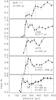 |
Fig. 3 Same as in Fig. 2 but for BHR 111, L328, L673, L1014 and L1148. |
| In the text | |
|
Fig. 4 The 2° × 3° extinction map produced by Dobashi et al. (2005) of the region containing IRAM 04191. The contours are drawn at 0.4, 0.6, 0.8, and 1.0 mag levels. The fields used for selecting star to determine distance are identified and labelled. The stars classified as dwarfs and used for determining distance to the cloud are identified using open circles. |
| In the text | |
|
Fig. 5 The AV vs. d plot for all the stars classified as dwarfs from the fields F1-2 combined together towards IRAM 04191. The dashed vertical line is drawn at 127 pc inferred from the procedure described in Sect. 2 (see Fig. 3). The dash-dotted curve represents the increase in extinction towards the Galactic latitude of b = −24° as a function of distance produced from the expressions given by BS80. The error bars are shown for a few stars to ensure that the data points can be seen more clearly. |
| In the text | |
|
Fig. 6 The ~3° × 4° extinction map produced by Dobashi et al. (2005) of the region containing L1521F. The contours are drawn at 0.5, 1.0, 1.5, 2.0, 2.5, and 3.0 mag levels. The fields used to select stars to determine distance are identified and labelled. L1521F is located in F3. |
| In the text | |
|
Fig. 7 The AV vs. d plot for all the stars classified as dwarfs from the fields F1-8 combined together towards L1521F. The dashed vertical lines are drawn at distances 116 pc and 156 pc inferred from the procedure described in Sect. 2 (see Fig. 3). The dash-dotted curve represents the increase in the extinction towards the Galactic latitude of b = −14.9° as a function of distance produced from the expressions given by BS80. The error bars are shown for only a few stars. |
| In the text | |
|
Fig. 8 The AV vs. d plot for the stars classified as dwarfs from the fields F1-4 in the upper panel and F5-8 in the lower panel towards L1521F. The dashed vertical lines are drawn at 116 pc and 156 pc. The dash-dotted curve represents the increase in the extinction towards the Galactic latitude of b = −14.9° as a function of distance produced from the expressions given by BS80. The error bars are shown for only a few stars. |
| In the text | |
|
Fig. 9 The ~1.5° × 1.5° extinction map produced by Dobashi et al. (2005) of the region containing BHR 111. The contours are drawn at 2, 2.1, 2.2, 2.3, and 2.4 mag levels. The fields used to select stars to determine distance are identified and labelled. The stars classified as dwarfs and used to determine distance to the cloud are identified using open circles. |
| In the text | |
|
Fig. 10 The AV vs. d plot for all the stars classified as dwarfs from the fields F1-3 combined together towards BHR 111. The dashed vertical line is drawn at 355 pc inferred from the procedure described in Sect. 2 (see Fig. 3). The dash-dotted curve represents the increase in the extinction towards the Galactic latitude of b = 1.824° as a function of distance produced from the expressions given by BS80. The error bars are shown for only a few stars. |
| In the text | |
|
Fig. 11 The AV vs. d plot for the stars classified as dwarfs from the individual fields F1, F2, and F3 towards BHR 111. The dashed vertical line is drawn at 355 pc inferred from the procedure described in Sect. 2 (see Fig. 3). The dash-dotted curve represents the increase in the extinction towards the Galactic latitude b = 1.824° as a function of distance based on the expressions given by BS80. The error bars are shown for only a few stars. |
| In the text | |
|
Fig. 12 The ~1° × 1° extinction map produced by Dobashi et al. (2005) of the region containing L328. The contours are drawn at 1.5, 2.0, 2.5, 3.0, 3.5, and 4.0 mag levels. The fields used to select stars to determine distances are identified and labelled. The stars classified as dwarfs using the near-IR photometry in each field are shown using filled circles. The fields F1 and F2 cover an area of 0.3° × 0.3° and 0.5° × 0.5°, respectively. |
| In the text | |
|
Fig. 13 The AV vs. d plot for all the stars classified as dwarfs from the fields F1 (open circles) and F2 (filled circles) combined together towards L328. The dashed vertical line is drawn at 217 pc inferred from the procedure described in Sect. 2 (see Fig. 3). The dash-dotted curve represents the increase in the extinction towards the Galactic latitude of b = −0.829° as a function of distance produced from the expressions given by Bahcall & Soneira (1980). The error bars are shown for only a few stars. |
| In the text | |
|
Fig. 14 The 1.5° × 1.5° extinction map produced by Dobashi et al. (2005) of the region containing L673-7. The contours are drawn at the 4.0 and 5.0 mag levels. The fields used to select stars to determine distances are identified and labelled. The stars classified as dwarfs using the near-IR photometry in each field are shown using filled circles. Each field covers an area of 0.5° × 0.5°. |
| In the text | |
|
Fig. 15 The AV vs. d plot for all the stars classified as dwarfs from the fields F1, F2 and F3 combined together towards L673. The dashed vertical line is drawn at 240 pc inferred from the procedure described in Sect. 2 (see Fig. 3). The dash-dotted curve represents the increase in extinction towards the Galactic latitude b = −1.33° as a function of distance based on the expressions given by BS80. The error bars are shown for only a few stars. |
| In the text | |
|
Fig. 16 The AV vs. d plot for the stars classified as dwarfs from the individual fields F1 (upper), F2 (middle), and F3 (lower panel) towards L673. The dashed vertical line is drawn at 240 pc inferred from the procedure described in Sect. 2 (see Fig. 3). The dash-dotted curve represents the increase in extinction towards the Galactic latitude b = −1.33° as a function of distance based on the expressions given by BS80. The error bars are shown for only a few stars. |
| In the text | |
|
Fig. 17 The 2° × 2° extinction map produced by Dobashi et al. (2005) of the region containing LDN 1148. The contours are drawn at 0.7, 1.0, and 2.0 mag levels. The fields used to select stars to determine distances are identified and labelled. Each field is of 0.7° × 0.7°. |
| In the text | |
|
Fig. 18 The AV vs. d plot for all the stars classified as dwarfs from the fields F1, F2, F3, and F4 combined together towards L1148. The dashed vertical lines are drawn at 168 pc and 301 pc inferred from the procedure described in Sect. 2 (see Fig. 3). The dash-dotted curve represents the increase in the extinction towards the Galactic latitude b = + 15.3° as a function of distance based on the expressions given by BS80. The error bars are shown for only a few stars. |
| In the text | |
|
Fig. 19 The AV vs. d plot for the stars classified as dwarfs from the individual fields F1 (open circles) and F2 (filled circles) in upper panel and F3 (filled circles) and F4 (open circles) in lower panel towards L1148. The dashed vertical lines are drawn at 168 pc and 301 pc inferred from the procedure described in Sect. 2 (see Fig. 3). The dash-dotted curve represents the increase in extinction towards the Galactic latitude b = + 15.3° as a function of distance based on the expressions given by BS80. The error bars are shown for only a few stars. |
| In the text | |
|
Fig. 20 The AV vs. d plot for the stars classified as dwarfs from the individual fields F5 (upper panel) and F6 (lower panel) towards NGC 7023. The dashed vertical lines are drawn at 168 pc, 310 pc, and 408 pc inferred from the procedure described in Sect. 2 (see Fig. 3). The dash-dotted curve represents the increase in extinction towards the Galactic latitude b = + 14.1° as a function of distance based on the expressions given by BS80. The error bars are shown for only a few stars to ensure that the points can be seen more clearly. |
| In the text | |
|
Fig. 21 The AV vs. d plot for all the stars classified as dwarfs towards L1122. The dashed vertical lines are drawn at 220 pc, 301 pc, and 408 pc. The dash-dotted curve represents the increase in extinction towards the Galactic latitude b = + 14.8° as a function of distance based on the expressions given by BS80. The error bars are shown for only a few stars to be able to distinguish more clearly between the points. |
| In the text | |
|
Fig. 22 The 1.2° × 1.2° extinction map produced by Dobashi et al. (2005) of the region containing L1014. The contours are drawn at 1.0, 1.5, and 2.0 mag levels. The fields used to select stars to determine distances are identified and labelled. The stars classified as dwarfs using the near-IR photometry in each field are shown using filled circles. Each field is of 0.4° × 0.4°. |
| In the text | |
|
Fig. 23 The AV vs. d plot for all the stars classified as dwarfs from the fields F1 and F2 combined together towards L1014. The dashed vertical lines are drawn at 221 pc and 258 pc inferred from the procedure described in Sect. 2 (see Fig. 3). The dash-dotted curve represents the increase in extinction towards the Galactic latitude b = −0.251° as a function of distance based on the expressions given by BS80. The error bars are shown for only a few stars to ensure more clarity in the presentation of the points. |
| In the text | |
Current usage metrics show cumulative count of Article Views (full-text article views including HTML views, PDF and ePub downloads, according to the available data) and Abstracts Views on Vision4Press platform.
Data correspond to usage on the plateform after 2015. The current usage metrics is available 48-96 hours after online publication and is updated daily on week days.
Initial download of the metrics may take a while.