| Issue |
A&A
Volume 536, December 2011
|
|
|---|---|---|
| Article Number | A52 | |
| Number of page(s) | 19 | |
| Section | Extragalactic astronomy | |
| DOI | https://doi.org/10.1051/0004-6361/201016031 | |
| Published online | 07 December 2011 | |
Molecular gas in the inner 0.7 kpc-radius ring of M 31
1
LERMA, Observatoire de Paris, LERMA, UMR 8112, 61 avenue de l’Observatoire, 75014 Paris, France
e-mail: This email address is being protected from spambots. You need JavaScript enabled to view it.
; This email address is being protected from spambots. You need JavaScript enabled to view it.
2
Université Pierre et Marie Curie-Paris 6, 4 place Jussieu, 75252 Paris Cedex 05, France
Received: 29 October 2010
Accepted: 6 September 2011
Abstract
The study of the gas kinematic in the central 1.5 kpc × 1.5 kpc region of M 31 has revealed several surprises. The starting point of this investigation was the detection at the IRAM-30 m telescope of molecular gas with very large line splittings up to 260 km s-1 within the beam (~40 pc). In this region, which is known for its low gas content, we also detect an ionised gas outflow in the circumnuclear region (within 75 pc from the centre) extending to the whole area in X-ray. Relying on atomic, ionised, and molecular gas, we account for most observables with a scenario that assumes that a few hundreds Myr ago, M 31 underwent a frontal collision with M 32, which triggered some star-formation activity in the centre, and this collision explains the special configuration of M 31 with two rings observed at 0.7 kpc and 10 kpc. The inner disc (whose rotation is detected in HI and ionised gas ([NII])) has thus been tilted (inclination: 43 deg, PA: 70 deg) with respect to the main disc (inclination: 77 deg, PA: 35 deg). One of the CO velocity components is compatible with this inner disc, while the second one comes from a tilted ring-like material with 40 deg inclination and PA = −35 deg. The relic star formation estimatedby previous works to have occurred more than 100 Myr ago could have been triggered by the collisionand could be linked to the outflow detected in the ionised gas. Last, we demonstrate that the amplitude of the line splittings detected in CO centred on the systemic velocity with a relatively high spatial resolution (40 pc) cannot be accounted for by a possible weak bar that is roughly aligned along the minor axis. Although M 31 has a triaxial bulge, there are no bar indicators in the gas component (photometry, no strong skewness of the isovelocities, etc.).
Key words: methods: data analysis / hydrodynamics / galaxies: ISM / Local Group / galaxies: bulges / molecular data
© ESO, 2011
1. Introduction
The merging processes that probably took place during the assembly of the galaxies of the Local Group is now actively studied (e.g., Klimentowski et al. 2010). While the Milky Way has not suffered any major merger for several billion years and presents only a series of dwarf galaxy stellar streams (see Helmi 2008), the other main spiral of the Local Group (M 31) has had a more perturbed history. Giant stellar loops and tidal streams are observed in the surroundings, extending up to the neighbour M 33, which is suspected to have interacted with M 31 (e.g., McConnachie et al. 2009). Many coherent structures observed around M 31 are interpreted as the disruption of small dwarf galaxies, which are numerous in the vicinity of M 31 (e.g., Ibata et al. 2004).
At the same time, it has been known for a long time that the M 31 galaxy exhibits an unusual morphology (e.g., Arp 1964; Haas et al. 1998; Helfer et al. 2003). The young stellar population tracers in the disc are all concentrated in the so-called 10 kpc ring(Chemin et al. 2009; Nieten et al. 2006; Azimlu et al. 2011), which is highly contrasted and superposed to only a few spiral structures(e.g., Nieten et al. 2006; Gordon et al. 2006). One striking feature is the small amount of gas present in the central region: neither Braun et al. (2009) nor Chemin et al. (2009) detect any significant HI component, while a similar depletion is observed in CO-emission by Nieten et al. (2006). It is usually described as a quiescent galaxy with little star formationSFR ~ 0.4 M⊙ yr-1 (e.g., Barmby et al. 2006; Tabatabaei & Berkhuijsen 2010; Azimlu et al. 2011) and with an ultra-weak nuclear activity (del Burgo et al. 2000). However, ionised gas is detected in the central field (e.g., Rubin & Ford 1971; Ciardullo et al. 1988; Boulesteix et al. 1987; Bogdán & Gilfanov 2008; Liu et al. 2010), usually interpreted in term of shocks, and Melchior et al. (2000) has detected only a small amount of molecular gas (1.5 × 10⁴ M⊙) within 1.3′ (305 pc in projection).There is no obvious on-going star formation in this central region (e.g., Olsen et al. 2006; Li et al. 2009; Azimlu et al. 2011) and the ionised gas (approximately 1500 M⊙ according to Jacoby et al. 1985) can be accounted for by mass lost from evolving stars.
Summary of observations.
In this “empty” central region, interest has focused on the supermassive black hole (Bacon et al. 1994),its activity (e.g., Li et al. 2011) and the circumnuclear region (inner few hundred parsecs)(Li et al. 2009). Barmby et al. (2006) observed the whole galaxy in the mid-infrared with the InfraRed Array Camera(IRAC) on board the Spitzer Space Telescope, revealing spectacular dust rings and spiral arms. Block et al. (2006) stress the presence of an elongated inner ring with projected diameters 1.5 kpc by 1 kpc and propose a completely new interpretation for the morphology of this galaxy. Both rings at 1 kpc and 10 kpc are off-centred. Their respective radii do not correspond to what is expected from resonant rings in a barred spiral galaxy. The most likely scenario for the formation of these rings is a head-on collision of the Cartwheel type(Struck-Marcell & Higdon 1993; Horellou & Combes 2001). Unlike the Cartwheel, where the companion is about 1/3rd of the mass of the target (major merger), in Andromeda, the collision can be called a minor merger, and produces much less contrasted rings in the main disc. Block et al. (2006) propose that the collision partner was M 32, with about 1/10th of the mass (dark matter included) at the beginning. After stripping experienced in the collision, the M 32 mass is now 1/23 that of the main target M 31. The M 32 plunging head-on through the centre of M 31 has triggered the propagation of an annular wave, which is now identified with the 10 kpc ring, and a second wave propagates more slowly behind (see e.g., Appleton & Struck-Marcell 1996), and would correspond to the inner ring. In addition, the inner ring has formed and is propagating in a tilted and warped disc, which accounts for its almost face-on appearance, in contrast with the inclined main disc of M 31. This scenario explains why the cold gas has been expelled from the central region and also why there are shocks and hot gas. In this article we focus on the gas content of the inner ring and inside.
We present CO(1 − 0) and CO(2 − 1) observations obtained with the IRAM-30 m telescope in different positions located in the north-western part of the inner ring, and a few positions inside the ring. While the CO intensities are correlated in first instance with the AB extinction, the velocity distributions are quite unexpected. In the inner ring the velocities are spread between − 450 kms-1 and − 150 kms-1 for a few positions while the systemic velocity (−310 kms-1) is expected in this area along the minor axis. To better understand these velocities, we compared our measurements with the velocities available for the ionised and HI gas and found that they do not really match. While neither the main HI warp of the disc nor a bar along the line of sight can explain the wide amplitude velocity splittings observed along the minor axis, the main configuration compatible with the data discussed here is to have a ring inclined with respect to the nuclear disc that would correspond in projection to the inner dust ring, which is detected in extinction and in infra-red emission. This ring could be attributed to a head-on collision with M 32 (Block et al. 2006) or to some accretion of gas from an M 31 − M 33 gas bridge or tidal loop detected in HI (Braun & Thilker 2004).
In Sect. 2 we describe the observations performed at the IRAM-30 m telescope. In Sect. 3 we describe the reduction of the CO data. In Sect. 4 we present an analysis of the CO data and compare the molecular gas with the ionised gas, together with information from other wavelengths. In Sect. 5 we explore various scenarios and propose one modelling that explains the observations. In Sect. 6 we discuss our results and conclude.
2. Observations
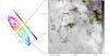 |
Fig. 1 Right: positions (J2000) observed in CO in the central part of M 31.
The circles indicate 1-mm (green) and 3-mm (red) beams of the 10 positions observed
superimposed on the AB extinction map
obtained in Melchior et al. (2000). As
discussed in this paper, the extinction with the central 2 arcsec is not well-defined
on this map. The (blue) cross indicates the centre of M 31 ( |
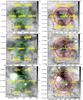 |
Fig. 2 Small maps performed at in CO(2 − 1) (left panels) and CO(1−0) (right panels) for the positions A, D and G. The green (resp. red) circles correspond to the FWHM of the CO(2−1) (resp. CO(1−0)) beams at the various positions observed. The corresponding offsets are: (0, 0), (+5, 0), (+2, +4) (−2, +4), (−5, 0), (−2, −4), (+2, −4). The spectra are superimposed on the corresponding AB maps. They are positioned arbitrarily close to the beam corresponding to the observations. |
The observations were carried out on 1999 June 13−15 and 2000 July 14−17 with the IRAM 30-m telescope. Most of the observations was made in the symmetrical wobbler switching mode, in which the secondary mirror nutates up to a maximum limit of ±240 arcsec in azimuth. The beam throw was determined as a function of the hour angle in a way that the OFF positions lay in extinction-free regions, as described in Melchior et al. (2000). It nevertheless occurred in two positions (M 31D and M 31G) that some signal was detected in the wobbler throw positions. As discussed in the Appendix A and indicated in Table 1, this corresponds to some azimuth angles for M 31G where one of the beam throws was close to the inner spiral arm in the north/north-western part of the field. For M 31Dthe configuration could be more subtle andthe OFF signal might have been caused by gas located on the far side, which was not detected in extinction. In the reduction process, the OFF signal is smeared out in the averaging process because equal weights are taken to reduce the observations to an equivalent beam of 24′′. It is still noticeable in M 31G because the OFF signal was also present in the 2000 observations. Near transit we had to use position-switching mode, taking an extinction-free OFF position located at a given position from the nucleus as indicated in the last column of Table 1. We found the OFF signal for M 31C for position-switch observations, while no ON signal has been detected. These OFF detections are presented in Appendix A.
During the second epoch of observations small maps of seven points with a spacing of 5′′ were made for positions (A, C, D and G) to sample the CO(1−0) beam in CO(2−1) and to compute the CO(2−1)/CO(1−0) line ratio. Pointing and focus calibration were regularly checked. In total, 10 ON positions in the inner disc of M 31 were observed in this way, as summarised in Table 1 and presented in Fig. 1. Table 1 provides (1) the name of the position observed, as used throughout the article, (2) the position angle in degrees of this position, (3) the offset in arcsec of the ON position with respect to the centre of M 31, (4) the distance R of this position with respect to the centre of M 31, (5) the right ascension, (6) the declination of this ON position, (7) the dates when the observations were made, (8) the total integration time on the source Texp, (9) if a small map (seven pointings) was made for this position, (10) if some signal was detected in the OFF position, if yes, WSW (resp. PSW) indicates that some OFF signal was detected in the wobbler (resp. position) switch scans performed for this position, (11) the offsets in arcsec used for position-switch observations made near transit.
We used four receivers simultaneously, two for 12CO(1 − 0) at 115 GHz and two for 12CO(2 − 1) at 230 GHz. At 115 GHz each receiver was connected to two autocorrelator sub-bands (shifted by 40 MHz from each other) and each sub-band consisted of 225 channels separated by 1.25 MHz. At 230 GHz each receiver was connected to a filter-bank consisting of 512 channels of 1 MHz width.
Characteristics of the CO lines. CO(2 − 1) (resp. CO(2 − 1)) spectra are reduced to a 2.6 kms-1 (resp. 3.2 kms-1) resolution.
3. Data reduction
The class1 package was used for the data reduction. After checking the quality of each single spectra, the data were averaged with inverse variance weights. A first-order baseline was fitted to the resulting spectrum and subtracted. For a few spectra, a higher-order polynomial was carefully subtracted. Finally, the spectra were smoothed to a velocity resolution of 3.2 kms-1 (resp. 2.6 kms-1) in CO(1 − 0) (resp. CO(2 − 1)).
The maps are presented in Fig. 2 and illustrate the observing procedure. The spectra are located arbitrarily close to the beam position they correspond to. Spatial variations in the spectra agree relatively well with the extinction distribution. For M 31G the CO intensity is clearly stronger in the area where the extinction is stronger. For M 31A and M 31D the intensity of the lines does not follow the intensity of the extinction exactly but we cannot exclude that some pointing errors and/or a clumpy distribution of the underlying gas explains the spatial variations of the CO distribution.
The results of the fitting are presented in Table 2. A Gaussian function is fitted to each line to determine its area, central velocity V0, width σ, and peak temperature Tpeak. The baseline RMS is provided for each line. We provide main-beam temperatures (unless specified otherwise) throughout this paper with Beff = 64.2 ± 3 and Feff = 91 ± 2 (resp. Beff = 42. ± 3 and Feff = 86 ± 2) at 115 GHz (resp. 230 GHz). For the positions for which maps have been observed, the spectra were convolved to obtain an 24″ beam  for both lines, enabling a direct computation of the line ratio.
The spectra are displayed in Fig. 3. In the final spectra, the signal present in the OFF positions is mainly visible for the position M 31G. It is at the systemic velocity and probably corresponds to the gas in the main disc along the minor axis in the north of the M 31G position (because the OFF positions are symmetric in azimuth with respect to the ON position). We use probably throughout this paper except for the Saglia et al. (2010) data, whose velocities are formally in LSR, but the difference (~5 km s-1) is negligible here.
 |
Fig. 3 Spectra with a detected signal. M 31A, M 31D and M 31G (resp. M 31E, M 31F, M 31I and M 31J) spectra are reduced to a 24″ beam (resp. with the original beam) in CO(2 − 1) and CO(1 − 0). The y-axis provides the antenna temperature in K. |
4. Analysis
4.1. Characteristics of the CO emission and gas-dust connection
The CO gas, which we searched for and discuss in this paper, is located mainly around the minor axis of the main disc of M 31. The detected molecular gas complexes correspond to the strongest AB extinction complexes that we observed. For the positions without extinction (M 31GB), we detected no signal, while no line was detected in the centre either. For M 31E where the extinction is weak, we have a tentative detection at 4σ. The extinction was computed assuming a fraction of foreground light of x = 0 (see Melchior et al. 2000), which is probably correct for the north-western part, where we observed, because an inclination of 45 deg is usually assumed for the nuclear spiral (Ciardullo et al. 1988). We also computed the near-UV and far-UV extinction maps from archive GALEX data with the same method and found the same structures. In addition, we subtracted from the original GALEX images the bulge emission modelled in this way, and found no trace of UV emission in the inner ring.
The position M 31F, which exhibits a weak CO(1 − 0) signal with no detection in CO(2 − 1), corresponds to a position with low AB extinction. The other positions are detected with high signal-to-noise (S/N) ratios at least in CO(1 − 0). We computed the AB extinction values for each position convolved with the different beams, as provided in Table 3, and there is no one-to-one correspondence with the intensity of the detected CO. Figure 1 also shows that M 31D has a much stronger signal in CO than M 31A while its AB extinction is weaker. One plausible explanation could be that the dust clumps corresponding to M 31D do not lie in the same plane as M 31A: if the foreground light (x) exceeds 0, we have underestimated the extinction. Assuming the ICO/AB ratio measured for M 31A applies to M 31D, one would expect a peak intensity  for M 31D, but it is measured
  . This configuration corresponds to a fraction of light in front of the dust x = 0.72, meaning that M 31D lies on the back side of the bulge. It is also probable that the gas is very clumpy and that the non-linearity of the extinction somehow biases our AB estimate.
Our detections are concentrated in an area2 of 415 pc × 570 pc (in projection), located in the north-western part of the M 31 within 3.8 arcmin from the centre, corresponding to 880 pc (resp. 1.2 kpc if deprojected for a 45 deg inclination). While the area explored is quite localised, the detected velocities span from − 73 to − 413 kms-1, while velocities along the minor axis of a rotating disc are expected to be at the systemic velocity. M 31K is the only position exhibiting this expected velocity, as well as a component for M 31G, M 31I and M 31J, and possibly M 31D. Figure 4 shows a superimposition of the spectra obtained for M 31G, M 31I and M 31J (and reduced to a 24′′ beam): the various velocity patterns appear in each spectra with different relative intensities. Besides the velocity line detected at − 145 kms-1, a broadband signal is detected with velocities between − 450 and − 250 kms-1. As discussed below, this range of velocities cannot be explained by a single disc inclined at 45 deg in regular rotation, and they are the signature of a peculiar structure. The line widths of the detected lines are quite different from one location to another, suggesting a spatial extension of the emitting areas. We assume a Galactic XCO = NH2/ICO = 2.3 × 1020 cm-2 (K kms-1)-1 following Strong et al. (1988). For the positions where we did not detect any signal, we provide a 3σ upper limit based on the dispersion (rms) computed on the baseline. Some CO(2 − 1) measurements (M 31I, M 31J, M 31K) are at the limit of detection and are provided for a rough comparison with CO(1 − 0) measurements.
AB extinction derived from the map based on the Ciardullo et al. (1988) data as obtained in Melchior et al. (2000).
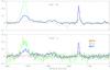 |
Fig. 4 Superimposition of the G, I, and J spectra at the nominal spatial resolution, namely 21″ for CO(1−0) and 11″ for CO(2−1). The y-axis provides the antenna temperature in K. |
In the centre (<2″), our AB map does not measure the extinction (owing to the method, which is based on ellipse fitting). The map of 8 μm emission (after subtraction of the scaled stellar continuum at 3.6 μm) also displays a defect in the central part, so it is difficult to be conclusive about the extinction in the inner arcseconds. However, Garcia et al. (2000), relying on simple modelling of Chandra data, have estimated AV = 1.5 ± 0.6 in the central 3-arcsec region. Our millimetre observations exclude the presence of CO(1−0) (resp. CO(2−1)) at the 1σ level of 3.7 mK (resp. 7.8 mK). On the basis of this upper limit, the gas present within 80 pc from M 31’s centre does not exceed 43 M⊙/pc-2 (3σ), assuming a conservative value for XCO typical of the Galactic disc. This is an extremely small amount compared to the gas mass computed in the central region of the Milky Way (Oka et al. 1998b).
Line ratios of the complexes reduced to a 24″ beam.
We used the three positions with observations reduced to a 24′′ beam to compute the CO(2 − 1) to CO(1 − 0) line ratio. As displayed in Table 4, we computed both the ratio of the integrated intensities and the ratio of the peak temperatures, which are compatible within error bars. M 31G exhibits a line ratio comparable with the mean value found for the Milky Way spiral arms (Sakamoto et al. 1997).
M 31A and M 31D exhibits CO line ratios higher than 1. Given the NH2 column densities computed (respectively 5.6 × 1020 cm-2 and 1.7 × 1020 cm-2), the gas is probably not optically thin. In addition, the velocity dispersion of CO(2 − 1) is systematically smaller than that of CO(1 − 0), suggesting that these complexes are probably externally heated and composed of dense gas. This hypothesis is compatible, as discussed below, with the combined presence of an intense stellar radiation field caused by bulge stars (Stephens et al. 2003), the outflow detected in X-ray in this area (Bogdán & Gilfanov 2008), and the ionised gas (Jacoby et al. 1985). This supports the view that no star formation is currently happening inside the inner ring of M 31.
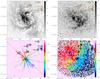 |
Fig. 5 Hα+[NII] (left) and [NII] (right) intensities from Ciardullo et al. (1988) and Boulesteix et al. (1987) are displayed with an arbitrary normalisation in the top panels. The bottom left panel presents the CO velocities measured in this paper, superimposed on the gas kinematics based on (1) Hβ and [Oiii] lines measured in slits by Saglia et al. (2010), (2) [Oii] and [Neiii] measured in slits by Ciardullo et al. (1988) and (3) Hα and [Nii] measured in slits by Rubin & Ford (1971). The bottom right panel displays the velocity field obtained with [Nii] λ6584 Ȧ observations (cf. top right panel) based on a Fabry-Perot device by Boulesteix et al. (1987). On each panel, the positions of our CO observations are indicated with circles corresponding to the beams. |
4.2. Ionised gas
The ionised gas in the central regions of M 31 has been mapped by Ciardullo et al. (1988), who produced the highest S/N ratio map of Hα+[NII] based on the compilation of a five-year nova survey published so far. It exhibits, as displayed in the top left panel of Fig. 5, a turbulent spiral, which appears more face-on than does the main disc. These authors described it as lying in a disc, warped in a way that the gas south of the nucleus is viewed closer to face-on than the gas in the northern half of the galaxy. As discussed in Block et al. (2006), this arc feature corresponds to the south-west part of the offset ring detected with Spitzer-IRAC data. Rubin & Ford (1971) measured that in this area [NII] is three times stronger than Hα, which supports the shock hypothesis as also discussed by Jacoby et al. (1985). According to Liu et al. (2010), half of the kinematic temperature of hot gas in the central bulge is accounted for by the stellar dispersion, but additional heating is expected from type-Ia supernovae, even though the question of the iron enrichment is not entirely clear. A head-on collision with M 32 suggested by Block et al. (2006) could account for the additional heating and at least contribute to it.
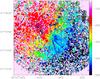 |
Fig. 6 6.7′ × 6.7′ ionised gas velocity field centred on M 31. Superimposition of the various gas velocities (see Fig. 5 bottom left) on the Boulesteix et al. (1987) Fabry-Perot-derived velocity map. |
In parallel, Boulesteix et al. (1987) observed this same area with a Fabry-Perot spectrograph to map the velocity field, and produced an [NII] map, which is displayed in the top right panel of Fig. 5. The centre has been masked for technical reasons. Besides the lower resolution and lower S/N ratio than for the Ciardullo et al. (1988) map (because of a smaller integration time), it is instructive to observe that it exhibits different patterns compared with the Hα+[NII] map. It is striking that the filament, which crosses the position M 31A, is not clearly detected in [NII], so it should be mainly associated to Hα component. The comparison of these two maps enhances the fact that obviously forbidden lines and Balmer lines do not sample exactly the same regions: (1) the gas does not have the same Hα/[NII] ratio everywhere; (2) the extinction additionally complicates the analysis.
4.2.1. Velocity field of the central bulge (1.5 kpc × 1.5 kpc)
To compare the ionised gas with our molecular detections, we tried to reconstruct the ionised gas velocity field from data published in the literature. Various lines have been used, but only a single velocity has been measured for each spectrum. In the bottom right panel of Fig. 5 we display the velocity map of Boulesteix et al. (1987). The best S/N ratio is of course observed where the [NII] intensity is strongest (cf. top right panel of Fig. 5). It exhibits an irregular disc in rotation, with obvious perturbations along the minor axis. Planetary nebulae are numerous in this field (537 detected by Merrett et al. 2006) and add noise to this velocity field. As discussed below (see Table 7), we estimate here a position angle of 70 deg ( − 20 deg for the kinematic minor axis) compared to 40 deg claimed by Boulesteix et al. (1987). Saglia et al. (2010) interpreted these perturbations as counter-rotations. In the bottom left panel of Fig. 5, we display the slit measurements we gathered from the literature, using Dexter3 when necessary, namely Hβ and [Oiii] from Saglia et al. (2010); [Oii] and [Neiii] from Ciardullo et al. (1988); Hα and [Nii] from Rubin & Ford (1971). We also superimpose our CO velocities, and find a very marginal agreement. In Fig. 6 we superimpose the two figures. We find a good overall agreement for the various ionised gas measurements with complicated features in the central part and along the minor axis, with the most striking discrepancy at position angles of 128 deg and 142 deg.
It is difficult to understand the discrepancies observed in the ionised gas velocity field, as the techniques are quite different and the Boulesteix et al. (1987) data suffers relatively low resolution (even though excellent given the fact that it has been obtained in 1985!). We can consider several explanations: (1) the various lines might have different relative ratios from one region to another (as seen in the top panels of Fig. 5) and might be affected differently by extinction (see Fig. 1); (2) it is possible that the ionised gas, like the molecular gas, exhibits several velocity components, and it has been not explored so far, but by Boulesteix et al. (1987), who mentioned line splittings greater than 30 kms-1 in the central region.
In addition, the CO velocities do not follow the regular pattern. M 31A and M 31D do not really match the ionised gas velocities. However, some CO positions might have a velocity (or at least one component) compatible with the ionised gas, namely M 31E, M 31F, M 31K, M 31I, M 31J and M 31G. This suggests that only part of the molecular gas is kinetically decoupled from the ionised gas.
Also, we wanted to figure out whether similar line splittings were present in the ionised data. As discussed by Saglia et al. (2010), the intrinsic velocity dispersions of the gas is smaller than 80 kms-1, while the instrumental resolution achieved by these authors is 57 kms-1. Boulesteix et al. (1987), who detected line splittings larger than 30 kms-1 in the central area, reached a spectral resolution of 14 kms-1. It is thus challenging to detect line splittings of this order of magnitude, but such splittings might be underlying and explain part of the discrepancies. As we observe large ( > 200 kms-1) line splittings in CO, we try to investigate if such double components can be detected from the ionised gas.
Line splittings detected on [Oiii] and Hβ lines from Saglia et al. (2010).
Optical spectra of M 31 are heavily dominated by the stellar continuum of its bulge. Therefore, in order to study emission lines in that spectral region we approximated the calibrated sky subtracted spectra of M 31 kindly provided by R. Saglia by stellar population models using the NBursts full spectral fitting technique (Chilingarian et al. 2007b,a). We excluded narrow regions around Hβ, [Oiii] , and [Ni] lines from the fitting. Then we subtracted the best-fitting stellar population models from the original spectra and analysed the fitting residuals. This allowed us to reliably measure parameters of these rather faint emission lines which are barely visible in the original data. We then inspect visually the spectra to determine the positions where high S/N line splittings is present. We then fit a two Gaussian functions with the CLASS package on the [Oiii] 5007 Ȧ line. Template mismatch and the relative low S/N affect the measurement of the Hβ, which is weaker and not always detected. For none of our measurements (but one), the [NI] line is detected. Our detection are summarised in Table 5 and Fig. 7. We identify 14 positions with a double component detected in [Oiii] and also in Hβ, within 23′′ (~86 pc) from the centre, but we do not detect any line splittings close to our CO observations or at a similar radial distance.
4.2.2. Velocity field of the circumnuclear region (150 pc × 150 pc)
Figure 7 displays the velocity field measured in ionised gas of the circumnuclear region. This includes slit data from Saglia et al. (2010) as well as two-dimensional spectroscopy of del Burgo et al. (2000) for the measurements of single velocity components, and our line splitting measurements based on Saglia et al. (2010) data. It is striking that unlike Fig. 6 this velocity field does not exhibit any clear rotation pattern in the central field. While the centre presents a spot at the systemic velocity, the whole area has velocities smaller than the systemic velocity and is approaching the observer. This coherent flow of ionised gas is decoupled from the stellar kinematics (e.g., Bender et al. 2005; del Burgo et al. 2000; Saglia et al. 2010), and resembles an ionised gas outflow. This is confirmed by the fact that the two independent data sets are in good agreement. We should stress that the Saglia et al. (2010) data are characterised by an instrumental resolution of 57 km s-1, and their systemic velocity is shifted by + 23 km s-1 with respect to the other studies. However, we checked that this cannot account for the systematic blue shift observed with respect to the centre. The mechanisms that rule the feed-back from the AGN are still largely unknown and in the case of M 31, we are only tracing a relic activity of its known black hole. Considering that M 31’s black hole is not active, two main mechanisms can be considered to explain this outflow. (1) It could be directly associated to the past stellar activity detected in the central regions: a 200 Myr old stellar disc with a 2400 M⊙ mass has been detected by Bender et al. (2005) within a fraction of arcsec from the centre. Inside a 2′′ disc, Saglia et al. (2010) has also detected a stellar component younger than 600 Myr corresponding to a mass smaller than 2 × 10⁶ M⊙: it could be compatible with a 100 Myr component with a mass of 106 M⊙. However, we lack of constraints to conclude for a star formation origin with a typical dynamic time τdyn = size/velocity of this outflow. The typical velocity of an outflow (e.g., Rupke et al. 2005) is about 400 km s-1, a τdyn = 100 Myr old starburst would then correspond to a size of the emitting area of 40 kpc. It might correspond to the X-ray outflow detected by Bogdán & Gilfanov (2008) (see Fig. 11, left panel). (2) As discussed by various authors (e.g., David et al. 2006; Ho 2009), the ionised gas in galaxy bulges can be accounted for by mass loss of evolved stars and SNIa could play a key role. The prompt SNIa component (which represents 50% of the SNIa population) discussed by Mannucci et al. (2006) could hence be indirectly linked to the 100 − 200 Myr star formation episodes quoted aboveand contribute to this outflow.
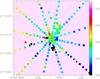 |
Fig. 7 40′′ × 40′′ ionised gas velocity field centred on M 31. Line splittings detected in [Oiii] 5007 Ȧ are superimposed on the velocity field measured on ionised gas by Saglia et al. (2010) and by del Burgo et al. (2000). This velocity field is quite unexpected and do not display any clear rotation pattern. |
As discussed in the following, a possible collision with M 32 can explain the ring structures of M 31 where the CO has been detected, and such an event could have triggered a star formation activity in the central part and support the SNIa explanation for the outflow. In addition, this inner outflow could be connected with the outflow detected in X-ray by (Bogdán & Gilfanov 2008) on a larger scale and discussed in Sect. 4.4.
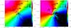 |
Fig. 8 Superposition of the various gas velocities (see Fig. 5 bottom left) (left:) on a simple model of a galactic disc with an inclination of 45 deg, a position angle of 40 deg and a systemic velocity of − 310 kms-1; (right:) similar disc with variable position angles. |
Several (8/14) of the positions with line splittings have a component with a large [Oiii] /Hβ ratio. Such a large ionisation is compatible with planetary nebulae. del Burgo et al. (2000) observed several high-ionisation “clouds” in this area. These authors discussed that the intensity of 3 of these sources is much larger than those of planetary nebulae detected in M 31 by Ciardullo et al. (2002). However, in this central region, it might be possible that these sources are multiple. Interestingly, one of the sources (D) detected by del Burgo et al. (2000) exhibits a line splitting ( − 270, − 527) km s-1 with an amplitude comparable with ours but very close to the centre, even though none of the velocities really match. Also, the strongest component we detect in the inner arcsec region matches in first approximation with the source A of del Burgo et al. (2000).
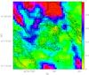 |
Fig. 9 Image of the HI emission in the very centre, avoiding ± 100 km s-1 around the systemic velocity of − 310 km s-1. This cut has been made to subtract the large-scale HI emission seen in projection superposed to the centre, expected near the systemic velocity. The contours are the dust emission from Spitzer-IRAC (8 μm image where a scaled version of the 3.6 μm image has been subtracted to remove the stellar photospheres emission) (Block et al. 2006). The HI cube is from Braun et al (2009). |
A comparison with SAURON data (M. Sarzi, priv. comm.) taken in this region of M 31 has shown that our multiple lines detections are compatible with planetary nebulae. The slit most probably biases the line ratio determination, as different parts of the PSF are sampled.
4.2.3. Modelling of a tilted inclined disc
We create a velocity field map with the CCDVEL task within the NEMO software package (Teuben 1995). Following Ciardullo et al. (1988), we consider a tilted ring model with an inclination of 45 deg, a position angle of 40 deg (Boulesteix et al. 1987) and a systemic velocity of − 310 kms-1. In order to understand the behaviour of the gas in the central part of M 31, we superimpose the velocities measured in this paper (ionised gas and CO gas) on this modelling in Fig. 8 (left panel). Even though there is a velocity field, as shown with ionised gas by Boulesteix et al. (1987) and displayed in the bottom right panel of Fig. 6, it is not regular and does not exhibit a well-defined zero-velocity curve. In addition, the velocities of the CO measurements do not fit with such a regular speed pattern. Varying the velocity angle in the centre, as displayed in the right panel of Fig. 8, mimics the velocity pattern in the inner region (<10 arcsec) but does not explain the minor axis configuration.
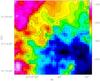 |
Fig. 10 Velocity field of the HI emission, corresponding to Fig. 9, avoiding large-scale HI emission. |
4.3. HI emission
The detailed maps from Braun et al. (2009) have revealed clearly the HI deficiency in the central parts of M 31. There is, however, some HI emission in the central kiloparsec, but most of it comes near the systemic velocity, and is likely to be projected emission from the external tilted gas orbits, which are warped to an almost edge-on inclination (e.g., Corbelli et al. 2010). To subtract this projected large-radii emission, and better see the residual coming from the actual centre, with a large velocity gradient, we have summed all channels avoiding ± 100 km s-1 around the systemic velocity of − 310 km s-1. A weak signal can then be distinguished, with a morphology of an incomplete ring (Fig. 9), with emission corresponding to the east side of the inner ring delineated by the dust emission revealed in the8 μm Spitzer-IRAC map. Figure 9 shows the dust contours superposed on the residual high-velocity central HI emission. In this picture, we can see that the main HI residual component still follows the large-scale (NE-SW) arms seen in projection, and coinciding with the dust features, in the direction of the major axis of M 31. However, there remains a weak component perpendicular (NW-SE) to it. The main concentration of this residual HI emission is well aligned with the north-east part of the dust ring and it could correspond to the weak component seen by Brinks (1983) on the minor axis position velocity diagram (his Fig. 1b). However, the remaining parts of the ring is devoid of HI emission; the atomic gas must have been transformed into the molecular phase in the dense parts of the ring. As discussed in Appendix B, Fig. B.1 reveals that most of the CO strong emission at high velocity in the centre has no HI counterpart.
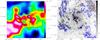 |
Fig. 11 Left: superposition of the Hα+ [Nii] map (upper left panel of Fig. 5) of Ciardullo et al. (1988) on the Chandra soft X-ray emission from Bogdán & Gilfanov (2008, see their Fig. 7). The Hα+ [Nii] map has been smoothed with the same smoothing lengths as those used for the Chandra map (A. Bogdan, priv. comm.). Right: superposition of the AB extinction on the 8 μm Spitzer-IRAC map after subtraction of a scaled version of the 3.6 μm image(Block et al. 2006). The AB contours are fixed to 0.05 (blue) and 0.15 (white). |
The HI component associated to the dust ring is, however, too weak to be seen in the velocity map, as shown from Fig. 10. The velocity field in the HI selected with high speed with respect to the systemic velocity, is still compatible to the “normal” main disc, and similar to the velocity field found with the ionised gas in Hα, although with possible perturbations in the vicinity of the ring. It is difficult to determine an accurate position angle of the HI isovelocity map (Fig. 10) to discriminate between the nuclear disc and the main disc, but the intensity map (Fig. 9) does not really favour a nuclear disc component.
4.4. Other wavelengths information
While the centre of M 31 hosts a massive black hole with a mass of 0.7 − 1.4 × 10⁸ M⊙ (Bacon et al. 2001; Bender et al. 2005), it is one of the most underluminous supermassive black hole (Garcia et al. 2010). The A-star cluster, detected in thethird component (P3) of M 31’s nucleus by Bender et al. (2005), can be associated to a recent star formation episode,typically a single burst, which occurred 200 Myr ago, with a total mass in the range 104 − 106 M⊙, corresponding to an accretion rate of 10-4 − 10-2 M⊙ yr-1. It might be triggered by the possible frontal collision with M 32 (Block et al. 2006). The detection of an ionised gas outflow in X-rays along the minor axis of the galaxy by Bogdán & Gilfanov (2008), perpendicular to the main disc, could be linked to this recent star formation activity and to the possible outflow detected in the optical (Fig. 7). However, this is still controversial as such a burst does not have enough energy to power the galactic wind required (Bogdán & Gilfanov 2008). In the left panel of Fig. 11, Hα + [Nii] contours are superimposed (with the same resolution) on the Chandra soft X-ray emission map from Bogdán & Gilfanov (2008). The relative intensity of the outflow on both sides is compatible with the intensity of AB extinction: the NW side is more extinguished than the SE side. This is compatible with the modelling described in the next section. Last, the right panel of Fig. 11 displays superimposition of the contours of the AB extinction map on the PAH-dust emission at 8 μm detected by Spitzer. The extinction features match exactly the ring detected at 8 μm.
5. Interpretation
The molecular, atomic and ionised gas exhibit different radial distributions in disc galaxies as first discussed by Kennicutt (1989; see also Bigiel et al. 2008, for a recent review). The HI gas is known to extend at much larger radius. M 31 has HI gas extending at least up to 40 kpc (Corbelli et al. 2010; Chemin et al. 2009) with high velocity clouds up to 50 kpc (Westmeier et al. 2008). As discussed below, the projected warp dominates the HI emission in the central part (see also B). The CO and ionised gas are usually more concentrated. In M 31, while CO is known to be depleted in its centre (Nieten et al. 2006), the ionised gas is detected in the inner parts (Ciardullo et al. 1988; Boulesteix et al. 1987) and is strongest there (Devereux et al. 1994).
While the atomic and ionised gas exhibit the presence a perturbed disc, the molecular gas detected in CO displays unexpected kinematic signatures, with significant line splits close to the minor axis and a very weak when present signal close to the systemic velocity. Several scenarios could be invoked to explain the existence of two well separated high S/N velocity components (ΔV = 260 kms-1 on a scale of 40 pc) traced by the molecular component (CO emission) in the centre of M 31. One component is in the sense of the expected rotation, the other component is counter-rotating. The widths of these two components are also very different, as displayed in Figs. 3 and 4.
The ionised gas also exhibits unexpected kinematic features with a face-on outflow in the circumnuclear region (detected in the optical), extending (in X-ray) to the 1.5 kpc × 1.5 kpc region studied in this paper.
In the following, we explore several possible scenarios to explain the observations. In Sect. 5.1, we discuss the expected effects of a large scale warp. In Sect. 5.2, we summarise the expected signatures of a bar and demonstrate that they fail to match the CO observations. In Sect. 5.3, we remind the scenario of a head-on collision with M 32 as proposed by Block et al. (2006) and show with a simple modelling that it can account for the various observables.
5.1. Scenario 1: large scale structures warp and tidal streams
We discuss the arguments that the second velocity component detected in CO could be due to the superimposition of gas at large scale onto the central regions. These possible configurations are not related to the outflows detected there in the ionised gas.
5.1.1. Large scale warp
We could think that the second component, the counter-rotating one, is just observed in projection, and comes from the external warp observed in the outer parts of the M 31 disc, with a different inclination and position angle than the normal M 31 disc. The warp is visually conspicuous, and remarkable in HI (Corbelli et al. 2010). Farther in the north-east disc (beyond 10 kpc), Casoli Combes (1988) already noted that CO emission could come from the main disc and the warped component, both on the same line of sight. In that case, the CO emission ( mK) was coming from material distant by more than 16 kpc from the centre.
This scenario is, however, impossible, because (1) the expected molecular gas has negligible emission at the large radii where this warped component should be (e.g., Neininger et al. 1998); (2) the corresponding projected velocity on the line of sight close to the centre is expected around the systemic velocity. It is likely that the gas at long distance (16 − 30 kpc) is on nearly circular orbits and has no radial velocity when projected to the centre. Accordingly, the corresponding warped material was always found at systemic velocity. Whatever inclination it has, the gradient in velocity across a small region of 40 pc should be negligible. Ad hoc hypotheses with HI infall/outflow with important radial velocity are then required, which are incompatible with the HI observations (e.g., Corbelli et al. 2010). We therefore think that, unless the gas is completely out of equilibrium (which is not really supported by the observations of Corbelli et al. 2010; Casoli Combes 1988), the peculiar component cannot come from the outer warp. However, we have some tentative detections close to the systemic velocity (M 31K, M 31I, M 31G, M 31J), which could be accounted for by the external warp. Some positions (e.g., M 31G) suffer from signal subtraction caused by the off positions (wobbler mode of observation), and we cannot exclude that the real signal could be a bit larger.
5.1.2. Large-scale tidal streams
The velocity range measured in CO is comparable with the measurements performed by Ibata et al. (2004); Chapman et al. (2008) for stellar streams and for extra-planar gas and high-velocity clouds detected in HI outside the disc (Braun & Thilker 2004; Westmeier et al. 2008). Casoli Combes (1988) have detected CO up to 16 kpc. Braun & Thilker (2004) detected a faint bridge of HI emission which appears to join the systemic velocities of M 31 with that of M 33 and continues beyond M 31 to the north-west. Davies’s cloud (Westmeier et al. 2008) lies in the north-west part of M 31’s disc and could belong to this bridge. Similarly to the stellar streams observed in the south-east part of M 31’s disc (Ibata et al. 2007), the HI gas exhibits large design loop-like features (e.g., the Magellanic stream, Kalberla & Haud 2006). The second component detected in the molecular gas we have detected could be associated to the M 31 − M 33 bridge or any gaseous-loop relics. It would then correspond to some accretion of gas onto the disc, generating an inner polar ring and leading to compression and excitation of the CO. This configuration can be compared to the inner polar gaseous disc discussed by Sil’chenko et al. (2011) in NGC 7217, where the disc is face-on.
While HI studies mention contamination by the Galaxy (Westmeier et al. 2008), our CO detections are related to extinction patterns that are clearly associated to M 31. The CO detected for M 31D has a mean velocity of − 74 kms-1 is typically below the limit for Galactic contamination used for HI. However, the typical velocity dispersion of HVC in the Galaxy is 8.5 kms-1, while the dispersion measured for M 31D is 24 kms-1. Furthermore, it exhibits a higher than expected ICO/E(B − V) ratio, rather suggesting that it lies behind the bulge and not in front of it. Finally, no CO from the Milky Way has been detected by Dame et al. (2001) in the vicinity of M 31.
Last, we cannot exclude that some non-circular velocities detected in CO result from relics of M 31’s formation: scattered debris or other extra-planar gas.
5.2. Scenario 2: a possible bar
Another a priori plausible scenario could be that the second velocity component is associated to a possible bar. Bars are frequent in spiral galaxies (60 to 75% are barred according to the bar strength; e.g., Verley et al. 2007), and it is likely that M 31 is barred or has been barred, because of its triaxial boxy bulge (Beaton et al. 2007). However, up to now, the bar is not visible in the gas in either the morphological or kinematical data.
5.2.1. Previous bar propositions in M 31
There have been several propositions of bar models for M 31. However, they are all contradictory (orientation of the bar along the minor axis or the major axis), and there is no coherent model that fits the observations. Stark & Binney (1994) assume the existence of a Ferrers bar potential in the centre to explain some non-circular motions there, but there was no complete velocity field, and they do not try to fit the observed stellar distribution with a bar. Their main point is to propose that the morphology of the gas in the centre of M 31 looks round,in spite of the bar, because of the high (77°) inclination of M 31: the bar would be aligned along the minor axis. The x1 orbits, elongated along the bar, i.e. the minor axis, are then projected as almost round, because their axis ratio could be as high as 4.44 = 1/cos(77°). The authors propose x1 orbits between 0.7 and 3 kpc in radius, and perpendicular x2 orbits inside 0.7 kpc. The gas would be shocked at the transition between x1 and x2 orbits, in a ring of 0.7 kpc radius. However, as is demonstrated below in Sect. 5.2.2, this scenario cannot account for the large observed velocity splitting along a single line of sight on the minor axis, at ~3.5 kpc from the centre.
Athanassoula & Beaton (2006) investigate the twist of isophotes of the NIR 2MASS image, which shows a boxy shape bulge. They compare this morphology with simulated stellar models with bars, without gas. They conclude that the NIR morphology of M 31 in the centre favours a bar, seen almost side-on, i.e. the angle between the bar and the major axis of the galaxy is between 20 and 30°. The size of the boxy-bulge is 1.4 kpc in radius, and the total length of the bar would be 4 kpc in radius, because a thin bar is identified beyond the boxy bulge (Beaton et al. 2007).
Let us note that in these two above propositions, the bar almost end-on, or almost side-on, there is no large angle between the bar and the symmetry axes of the projected galaxy (major or minor axis). This is required because of the morphological symmetry of the disc (no bar is obvious in the gas), and also because of the fairly regular velocity field. If the bar were inclined by ~45° with respect to the major axis, strongly skewed (S-shape) isovelocities should be seen in the gas, i.e. the kinematical minor axis would not be perpendicular to the major axis, as in N2683 (Kuzio de Naray et al. 2009), which has been compared to M 31. In the latter, owing to the relative deficiency of gas in the centre (Brinks & Shane 1984; Nieten et al. 2006), it is difficult to trace isovelocities, but Figs. 6 and 10 reveal that there is no strong skewness.
Athanassoula & Beaton (2006) also present a 2D gaseous velocity field in an analytical bar potential (not fitted to M 31) and project it edge-on, i.e. all regions of the galaxy up to 20 kpc can thus be seen artificially on the same line of sight, which makes a big difference from a 77° projection corresponding to M 31’s real configuration. The model 2D gas morphology clearly shows a bar, with emptied regions that are not similar to the de-projected view of M 31 gaseous disc (e.g., Braun 1991). The authors compare the position-velocity diagrams parallel to the major axis that they derived from the 2D-edge-on model to those observed in HI. The latter reveal conspicuous figure-eight shapes that turn at the end of the HI extent (R = 70′ ~ 15 kpc), and have been interpreted as caused by the warp (Henderson 1979; Brinks & Burton 1984). These features are much larger than the (3 − 4 kpc) bar extent. Note that in the galaxy NGC 2683, as inclined on the sky plane as M 31, the position-velocity diagram along the major axis is not a figure-eight shape, but a parallelogram that ends at a certain radius, precisely the radius of the bar R = 2.2 kpc = 45″ (Kuzio de Naray et al. 2009). The situation is completely different in M 31.
5.2.2. Special case of M 31
Is it possible to obtain two velocity components on each side of the systemic velocity along the same line of sight, near the minor axis (position of M 31-I and J), at a distance of 210 arsec, i.e. 3.5 kpc from the centre (if the points are in the main inclined plane)? The possibility to gather several components in the same beam strongly depends on the spatial resolution. Here, the CO(2 − 1) beam is 12″ ~ 40 pc on the major axis, however, the inclination of the plane limits the resolution. Typically, gaseous discs in the centre of galaxies have a characteristic scale-height of 50 pc, as determined in the Milky Way (e.g., Sanders et al. 1984). The inclined line of sight across the disc of M 31 encompasses a region of size = tan(77°) × 50 pc = 216 pc in the direction parallel to the minor axis (while it is the size of the beam, 40 pc, in the perpendicular direction). The region explored in one line of sight then goes along the minor axis from 3.4 kpc to 3.6 kpc, and only 40 pc in the perpendicular direction. The only place where it would be possible to have two velocity components on each side of the systemic velocity is the very centre, because the 216 pc region explored would encompass the two sides of an elongated orbit. Assuming that the bar is inclined with some angle with respect to the major axis, the elongated orbits will provide red- and blue-shifted velocities on each side of the centre. This is the case in NGC 2683 for instance, which is revealed by a long slit exactly along the major axis. It is possible in the centre, because the bar is inclined with respect to the symmetry axes. However, at a distance of 3.5 kpc from the centre ( ± 100 pc), it is impossible to obtain these two V-components, with the same category of orbits, either x1 or x2. The only other possibility so far from the centre would be to consider a change of orientation in the orbits, or a sudden shock, as occurs from x1 to x2, or crossing an arm. However, the amplitude of the shock, 260 km s-1, and the positions of the two components on the two sides of Vsys is unrealistic, especially for a possible weak bar.
5.2.3. Examples of bar shocks
Several strongly barred galaxies have been studied in Hα spectroscopy, determining the kinematics with high spatial resolution, comparable to what we have in the CO gas towards M 31. NGC 1365 is the prototype of a very strong bar. The position angle of the bar does not coincide with the symmetry axis of the projection, so that the bar signatures are obvious. With an inclination of i = 42°, and a distance of D = 20 Mpc, the observed velocity gradient across the bar dust lanes is determined to be at maximum 40 kms-1, with a spatial resolution below 100 pc (Lindblad et al. 1996). If deprojected, the maximum would be 60 kms-1. NGC 1300 is another remarkable and strongly barred spiral galaxy, where the kinematics has been studied in detail in Hα, on scales smaller than 100 pc. Lindblad et al. (1997) present a projected velocity gradient across the dust lanes with shocks of 20−30 kms-1 projected on the sky. When deprojected, this becomes a maximum of 35−50 kms-1. To reach these strong velocity gradients, a highly contrasted gas structure must be found, which is not the case for the M 31 central region.
In the molecular component, interferometric observations of nearby barred galaxies can now yield sub-arcsec resolution, corresponding to scales smaller than 100 pc, therefore comparable to the single-dish resolution towards M 31. García-Burillo et al. (2005) have presented non-circular motions caused by bars, which are of the same orders of magnitude ~60−70 kms-1. More recently, with even higher sensitivity and resolution, van der Laan et al. (2011) have for the first time seen dedoubled velocity profiles in the CO data towards the barred galaxy NGC 6951. If interpreted in terms of crowding of orbits, they reveal velocity differences of 80 kms-1 (within 500 pc), which in deprojection would amount to 110 kms-1. The CO velocity profiles are, however, very broad in the centre of this galaxy, showing a starburst ring, and it is not sure what is caused by turbulence or by the bar. The molecular gas surface density in the centre is on average 100 M⊙/pc2 (corresponding to a total mass of 1.5 × 10⁹ M⊙ inside 2 kpc), which may explain the unstable and turbulent gas-forming stars, while in M 31 the surface density is at least one order of magnitude lower. The velocity dispersion in the distinct velocity components observed in CO is quite low (15 kms-1), which corresponds to a stable gas layer. We conclude that the bar is not a likely explanation for the special kinematical phenomenon observed towards the M 31 centre.
5.2.4. Other interpretations
From the HI-derived gas morphology, Braun (1991) suggests a two-armed trailing density wave with a pattern speed of 15 kms-1 kpc-1, leading to a corotation at 16 kpc, an ILR at 5 kpc, and an OLR at 22 kpc. He proposes as the driver of the spiral structure the collision with M 32, which could also be responsible for the many tilts of the M 31 plane. The nearly head-on collision with M 32 has been developed in detail by Block et al. (2006), which allows them to account for the two off-centred gas rings observed in M 31 at 0.7 kpc and 10 kpc radius. Indeed, these authors note that the gas morphology in M 31 does not show the usual signatures of the response to a bar. Although it is possible that the galaxy disc possesses a stellar bar, aligned with the triaxial bulge, oriented roughly along the major axis, the observed 0.7 kpc dust ring is aligned almost along the minor axis, and not aligned with the potential bar along the major axis. The size of the inner ring does not correspond to a possible inner Lindblad resonance, nor the outer ring at 10 kpc radius to a correlated outer resonance. Moreover, the inner disc appears highly inclined with respect to the main disc, and the inner ring is off-centred by 40% of its radius, which is not expected in barred galaxies. This offset centre and the tilted plane of the inner disc strongly point towards a perturbed origin of the inner features of M 31.
5.3. Scenario 3: head-on collision with M 32
Jacoby et al. (1985) have shown that the inner disc of M 31 is tilted with respect to the main disc. While the inclination of the large-scale disc is 77°, the nuclear disc, of size ~1 kpc, is inclined by only about 40° on the sky plane. Block et al. (2006) discovered in the Spitzer-IRAC maps an inner dust disc of scale 1 kpc by 1.5 kpc, which also appears with this low inclination. The ring morphology of this tilted structure together with the ring (10 kpc) morphology of the large-scale disc led these authors to propose a head-on collision with a small companion, with a probable candidate being M 32.
In this scenario, we assume that the peculiar component comes from a tilted ring-like material, likely coming from the perturbed gas from the recent M 32 collision. The collision might have perturbed the nuclear disc, which was already tilted, and produced some local warp before the annular density wave propagated outwards. Besides its interest for the inner configuration of M 31, this scenario also proposes an explanation for the 10 kpc ring, resulting from the propagation of the initial annular wave.
The resulting configuration is similar to the scenario proposed in Sect. 5.1.2. Below, we discuss some modelling that enables one to explain the observations. We stress that this modelling is meant to be schematic rather than reproducing the observations in a fully self-consistent manner.
We used a model for the gas, through static simulations of dynamical components represented by particles, with different geometrical orientations on the sky, but embedded in a gravitational potential representing the observed rotation curve of M 31.
We represent the gaseous disc of M 31 by a fairly homogeneous Miyamoto-Nagai disc of particles (with radial scale of 1 kpc, and height of 0.2 kpc) to be able to vary easily the inclination and position angle as a function of radius. We used typically half a million particles to have sufficient statistics. We plunged the gas disc into a potential made of a stars and a dark matter halo. The stellar component is composed of a bulge and a disc. The bulge is initially distributed as a Plummer sphere, with a potential  (1)where Mb and rb are the mass and characteristic radius of the bulge, respectively (see Table 6).
The stellar disc is initially a Kuzmin-Toomre disc of surface density  (2)with a mass Md, and characteristic radius rd.
The dark matter halo is also a Plummer sphere, with mass MDM and characteristic radius rDM. A summary of the adopted parameters is given in Table 6. The resulting rotational velocity curve is rising until a maximum of 300 kms-1, reached at 3 kpc, and then slightly decreases, remaining close to 300 kms-1 in the central regions of interest here. This corresponds to the rotational velocity observed (e.g., Carignan et al. 2006). All molecular clouds we aim to reproduce are inside the radius of maximum rotational velocity.
The gas particles are distributed in this potential, with the velocity dispersion corresponding to a Toomre Q parameter of 1.3.
Model parameters.
To reproduce the observations, we adopted an inclination of 43° for the gaseous nuclear disc, inside the 1.5 kpc radius. At the boundary of this disc, we assumed a progressive warping of the disc plane, so that the inclination on the sky grows from 43 to 77 degrees, over 300 pc. The details of this transition, however, are not constrained by the observations, because the latter are all inside the 1 kpc radius. As for the position angle on the sky, the nuclear disc has PA = 70°, unlike the main disc, which has PA = 35°. In projection on the sky, the nuclear gas disc model gives velocities that agree with the observations, at least with the main velocity component. In many observed points only this main component is observed, with a broad line-width (FWHM = 50−70 kms-1), located on the blueshifted side in the SW and on the redshifted side in the NE of the major axis. In some of the points there is an additional peculiar velocity component, located on the opposite side (redshifted in the SW), and narrower (20 kms-1).
Trying several parameters, we found that material on a ring-like orbit, with 40° inclination, and PA = −35° gives kinematical features compatible with the observations (cf. Figs. 12−15). The modelled ring has a width of 0.4 kpc, and a mean radius of 0.6 kpc, coinciding with the observed dust ring. The adopted position angle and inclination of the various components are displayed in Table 7.
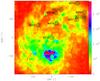 |
Fig. 12 Mean density of CO emission from the homogeneous nuclear disc plus tilted ring of the model. The field of view is 200 arcsec in radius, or 0.76 kpc in radius. The density scale, indicated in the wedge, is in arbitrary units. The positions of our CO observations are indicated with circles corresponding to the beams. |
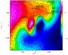 |
Fig. 13 Density-weighted mean velocity (first moment) of the simulated nuclear region in the same field of view as Fig. 12. Signatures of the tilted ring can be seen at the boarder of the field. The wedge gives the velocity scale inkms-1. |
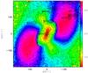 |
Fig. 14 Density-weighted velocity dispersion (second moment of the simulated velocity field). The wedge gives the velocity scale in kms-1. The locations of double components with counter-rotating features correspond to the blue and purple regions. |
Geometrical parameters.
To draw these maps, we built data cubes corresponding to the observations, with a pixel of 6 arcsec, and channels of 12 kms-1, and the data smoothed to a beam of 12′′. The pixel size of the cubes are therefore (60, 60, 40) to describe the inner parts studied here in CO lines and dust extinction. To take into account that the gas and dust distribution is not homogeneous, but patchy, we smoothed the dust map obtained by Block et al. (2006) from Spitzer-IRAC images (the 8 μm map with the 3.6 μm contribution subtracted) to the same spatial resolution, and used it as a multiplicative filter for our homogeneous disc map. This takes into account that the dust inner ring is offset by 0.5 kpc (131′′) from the centre of the galaxy.
Typical spectra were extracted in the zone where double features are expected at the offset indicated in Fig. 15 in arcseconds. On the one hand, the broad characteristics of the blue-shifted velocity component is caused by beam smearing of the velocity gradient, as illustrated here with a 12″ beam. On the other hand, because the ring is narrow in radius (~170 pc) and in a region of a flat rotation curve, the velocity gradient in the beam is very flat and a narrow line is observed in the redshifted component.
In addition, some emission at the systemic velocity is expected because of the inclination of the 77 deg main disc. It is therefore not necessary to evoke the large-scale warp to explain the weak emission at the systemic velocity, which can be accounted for by the inner main disc. For positions like M 31I/M 31J/M 31G located in the north-west ring, main disc regions at 3.5 kpc project in the same beam.
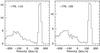 |
Fig. 15 Spectra extracted from the simulated cube at the (RA, Dec) offset in arcseconds indicated in each panel. The vertical scale is in arbitrary units. The velocities are centred at the systemic velocity. These offsets correspond the M 31G and M 31I positions. The clumpiness of the gas (not included in the modelling proposed here) is expected to modulate the relative intensity of the various components additionally. |
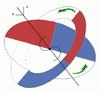 |
Fig. 16 Schematic view of the interpretation proposed for the CO velocities observed. The inner disc is presented with a PA of 70 deg and an inclination of 43 deg. The inner ring is superimposed with a similar inclination but a position angle of −35 deg. The straight line indicates the position of the major axis of the main disc inclined by 77 deg with a PA of 35 deg. The bars labelled “N” and “E” have a length of 150 pc. The near (resp. far) sides of the two components are coloured (resp. kept white). The red (resp. blue) colours correspond to the redshift (resp. blueshift) relative to the systemic velocity. |
6. Discussion and conclusions
We have detected CO emission, tracing the presence of molecular gas in several positions in the central kpc of M 31, corresponding to dust extinction. We have also shown that there is an excellent correspondence between the dust extinction measured in the optical and the dust emission in the near-infrared at 8 μm (right panel of Fig. 11). Some of the observed positions correspond to the conspicuous inner ring, detected in dust emission by IRAC on Spitzer (Block et al. 2006). This ring was also present in ISO data studied by Willaime et al. (2001) and in ionised gas maps as proposed by (Jacoby et al. 1985). The velocity information brought by the CO lines reveals a complex kinematical structure, different from the ionised and atomic gas dynamics. In the NW inner ring positions, two main high S/N velocity components are detected on each side of the systemic velocity. The component with the expected velocity, according to the rotation curve and the positive position angle, is broad, and is likely to correspond to the nuclear disc. Exploring a wide region of the strong central rotational gradient, the beam-averaged spectrum may be 100 km s-1 broad. The second component, redshifted on the other side of the systemic velocity, has a small velocity width, because it is not a full disc, but a relatively narrow ring. We used radii from 0.4 to 0.8 kpc for the model.
We summarise in Fig. 16 the geometry of the two components we propose in our modelling. The peculiar component appears to be counter-rotating, because the gas is in a tilted ring, almost perpendicular to that of the inner disc. Its inclination on the plane of the sky is similar, which explains why the amplitude of the projected rotation is the same as for the regular component. In the figure the arrows indicate the apparent sense of rotation. The two discs appear to rotate in the same direction, which is also that of the main M 31 disc. The apparent counter-rotation appears only in the NW (and SE) regions, where blue and red regions superpose. The winding sense of the spiral structure in the observations is also sketched. It is possible to see that the arms are trailing, exactly like the M 31 main disc.
In summary, the apparent counter-rotation is only caused by a warping and distortion of the central components, possibly triggered the proposed head-on collision with M 32, but is not a true counter-rotation.
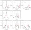 |
Fig. B.1 HI spectra obtained with a 1 arcmin resolution for the CO positions discussed in this paper. In each spectrum the velocity of the CO emission is indicated in red. |
Continuum and Line Analysis Single-dish Software, http://www.iram.fr/IRAMFR/GILDAS
As in Melchior et al. (2000), we assume a distance of M 31 of 780 kpc i.e. 1 arcsec = 3.8 pc.
Acknowledgments
We are most grateful to F. Viallefond, who designed the observing procedures and to M. Marcelin, who retrieved for us old kinematical [Nii] data. We thank R. Saglia who has kindly provided the slit spectra he took in the bulge, enabling us to search for double components and Á Bogdán for providing their reduced XMM-Newton and Chandra maps of the bulge exhibiting an X-ray outflow and helpful comments. We acknowledge I. Chilingarian for his help in the spectra reduction and M. Sarzi for helpful comments. We are very grateful to Robert Braun for his constructive comments, and for having provided the HI data, in order to check the HI correlation with the CO data. We thank the anonymous referee for his constructive remarks, which helped us to improve the manuscript. This paper is based on observations carried out with the IRAM 30 m telescope. IRAM is supported by INSU/CNRS (France), MPG (Germany) and IGN (Spain). The authors are grateful to the IRAM staff for their support.
References
- Appleton, P. N., & Struck-Marcell, C. 1996, FCPh, 16, 111 [Google Scholar]
- Arp, H. 1964, ApJ, 139, 1045 [NASA ADS] [CrossRef] [Google Scholar]
- Athanassoula, E., & Beaton, R. L. 2006, MNRAS, 370, 1499 [NASA ADS] [CrossRef] [Google Scholar]
- Azimlu, M., Marciniak, R., & Barmby, P. 2011, AJ, 142, 139 [NASA ADS] [CrossRef] [Google Scholar]
- Bacon, R., Emsellem, E., Monnet, G., & Nieto, J. L. 1994, A&A, 281, 691 [NASA ADS] [Google Scholar]
- Bacon, R., Emsellem, E., Combes, F., et al. 2001, A&A, 371, 409 [NASA ADS] [CrossRef] [EDP Sciences] [Google Scholar]
- Barmby, P., Ashby, M. L. N., Bianchi, L., et al. 2006, ApJ, 650, L45 [NASA ADS] [CrossRef] [Google Scholar]
- Beaton, R. L., Majewski, S. R., Guhathakurta, P., et al. 2007, ApJ, 658, L91 [NASA ADS] [CrossRef] [Google Scholar]
- Bender, R., Kormendy, J., Bower, G., et al. 2005, ApJ, 631, 280 [NASA ADS] [CrossRef] [Google Scholar]
- Bigiel, F., Leroy, A., Walter, F., et al. 2008, AJ, 136, 2846 [NASA ADS] [CrossRef] [Google Scholar]
- Block, D. L., Bournaud, F., Combes, F., et al. 2006, Nature, 443, 832 [NASA ADS] [CrossRef] [Google Scholar]
- Bogdán, Á., & Gilfanov, M. 2008, MNRAS, 388, 56 [NASA ADS] [CrossRef] [MathSciNet] [Google Scholar]
- Boulesteix, J., Georgelin, Y. P., Lecoarer, E., Marcelin, M., & Monnet, G. 1987, A&A, 178, 91 [NASA ADS] [Google Scholar]
- Boulesteix, J., Coarer, E. L., Marcelin, M., & Monnet, G. 1995, Astrophys., 38, 345 [NASA ADS] [CrossRef] [Google Scholar]
- Braun, R. 1991, ApJ, 372, 54 [NASA ADS] [CrossRef] [Google Scholar]
- Braun, R., & Thilker, D. A. 2004, A&A, 417, 421 [NASA ADS] [CrossRef] [EDP Sciences] [Google Scholar]
- Braun, R., Thilker, D. A., Walterbos, R. A. M., & Corbelli, E. 2009, ApJ, 695, 937 [Google Scholar]
- Brinks, E. 1983, IAUS, 100, 27 [NASA ADS] [Google Scholar]
- Brinks, E., & Burton, W. B. 1984, A&A, 141, 195 [NASA ADS] [Google Scholar]
- Brinks, E., & Shane, W. W. 1984, A&AS, 55, 179 [NASA ADS] [Google Scholar]
- Carignan, C., Chemin, L., Huchtmeier, W. K., & Lockman, F. J. 2006, ApJ, 641, L109 [NASA ADS] [CrossRef] [Google Scholar]
- Casoli, F., & Combes, F. 1988, A&A, 198, 43 [NASA ADS] [Google Scholar]
- Chapman, S. C., Ibata, R., Irwin, M., et al. 2008, MNRAS, 390, 1437 [NASA ADS] [Google Scholar]
- Chemin, L., Carignan, C., & Foster, T. 2009, ApJ, 705, 1395 [NASA ADS] [CrossRef] [Google Scholar]
- Chilingarian, I., Prugniel, P., Sil’chenko, O., & Koleva, M. 2007a, in Stellar Populations as Building Blocks of Galaxies, ed. A. Vazdekis & R. R. Peletier (Cambridge, UK: Cambridge University Press), IAU Symp., 241, 175 [Google Scholar]
- Chilingarian, I. V., Prugniel, P., Sil’chenko, O. K., & Afanasiev, V. L. 2007b, MNRAS, 376, 1033 [NASA ADS] [CrossRef] [Google Scholar]
- Ciardullo, R., Rubin, V. C., Ford, W. K., Jr., Jacoby, G. H., & Ford, H. C. 1988, AJ, 95, 438 [NASA ADS] [CrossRef] [Google Scholar]
- Ciardullo, R., Feldmeier, J. J., Jacoby, G. H., et al. 2002, ApJ, 577, 31 [NASA ADS] [CrossRef] [Google Scholar]
- Corbelli, E., Lorenzoni, S., Walterbos, R., Braun, R., & Thilker, D. 2010, A&A, 511, A89 [NASA ADS] [CrossRef] [EDP Sciences] [Google Scholar]
- Crane, P. C., Dickel, J. R., & Cowan, J. J. 1992, ApJ, 390, L9 [NASA ADS] [CrossRef] [EDP Sciences] [Google Scholar]
- Dame, T. M., Hartmann, D., & Thaddeus, P. 2001, ApJ, 547, 792 [NASA ADS] [CrossRef] [Google Scholar]
- David, L. P., Jones, C., Forman, W., Vargas, I. M., & Nulsen, P. 2006, ApJ, 653, 207 [NASA ADS] [CrossRef] [Google Scholar]
- del Burgo, C., Mediavilla, E., & Arribas, S. 2000, ApJ, 540, 741 [NASA ADS] [CrossRef] [Google Scholar]
- Devereux, N. A., Price, R., Wells, L. A., & Duric, N. 1994, AJ, 108, 1667 [NASA ADS] [CrossRef] [Google Scholar]
- Garcia, M. R., Murray, S. S., Primini, F. A., et al. 2000, ApJ, 537, L23 [NASA ADS] [CrossRef] [Google Scholar]
- Garcia, M. R., Hextall, R., Baganoff, F. K., et al. 2010, ApJ, 710, 755 [NASA ADS] [CrossRef] [Google Scholar]
- García-Burillo, S., Combes, F., Schinnerer, E., Boone, F., & Hunt, L. K. 2005, A&A, 441, 1011 [NASA ADS] [CrossRef] [EDP Sciences] [Google Scholar]
- Gordon, K. D., Bailin, J., Engelbracht, C. W., et al. 2006, ApJ, 638, L87 [Google Scholar]
- Haas, M., Lemke, D., Stickel, M., et al. 1998, A&A, 338, L33 [NASA ADS] [Google Scholar]
- Helfer, T. T., Thornley, M. D., Regan, M. W., et al. 2003, ApJS, 145, 259 [NASA ADS] [CrossRef] [Google Scholar]
- Helmi, A. 2008, A&AR, 15, 145 [NASA ADS] [Google Scholar]
- Henderson, A. P. 1979, A&A, 75, 311 [NASA ADS] [Google Scholar]
- Ho, L. C. 2009, ApJ, 699, 638 [NASA ADS] [CrossRef] [Google Scholar]
- Horellou, C., & Combes, F. 2001, Ap&SS, 276, 1141 [NASA ADS] [CrossRef] [Google Scholar]
- Ibata, R., Chapman, S., Ferguson, A. M. N., et al. 2004, MNRAS, 351, 117 [Google Scholar]
- Ibata, R., Martin, N. F., Irwin, M., et al. 2007, ApJ, 671, 1591 [NASA ADS] [CrossRef] [Google Scholar]
- Jacoby, G. H., Ford, H., & Ciardullo, R. 1985, ApJ, 290, 136 [NASA ADS] [CrossRef] [Google Scholar]
- Kalberla, P. M. W., & Haud, U. 2006, A&A, 455, 481 [NASA ADS] [CrossRef] [EDP Sciences] [Google Scholar]
- Kennicutt, R. C., Jr. 1989, ApJ, 344, 685 [NASA ADS] [CrossRef] [Google Scholar]
- Klimentowski, J., Łokas, E. L., Knebe, A., et al. 2010, MNRAS, 402, 1899 [NASA ADS] [CrossRef] [Google Scholar]
- Kuzio de Naray, R., Zagursky, M. J., & McGaugh, S. S. 2009, AJ, 138, 1082 [NASA ADS] [CrossRef] [Google Scholar]
- Li, Z., Wang, Q. D., & Wakker, B. P. 2009, MNRAS, 397, 148 [NASA ADS] [CrossRef] [Google Scholar]
- Li, Z., Garcia, M. R., Forman, W. R., et al. 2011, ApJ, 728, L10 [NASA ADS] [CrossRef] [Google Scholar]
- Lindblad, P. O., Hjelm, M., Hoegbom, J., et al. 1996, A&AS, 120, 403 [NASA ADS] [CrossRef] [EDP Sciences] [Google Scholar]
- Lindblad, P. A. B., Kristen, H., Joersaeter, S., & Hoegbom, J. 1997, A&A, 317, 36 [NASA ADS] [Google Scholar]
- Liu, J., Wang, Q. D., Li, Z., & Peterson, J. R. 2010, MNRAS, 404, 1879 [NASA ADS] [Google Scholar]
- Mannucci, F., Della Valle, M., & Panagia, N. 2006, MNRAS, 370, 773 [NASA ADS] [CrossRef] [Google Scholar]
- McConnachie, A. W., Irwin, M. J., Ibata, R. A., et al. 2009, Nature, 461, 66 [NASA ADS] [CrossRef] [PubMed] [Google Scholar]
- Melchior, A.-L., Viallefond, F., Guélin, M., & Neininger, N. 2000, MNRAS, 312, L29 [NASA ADS] [CrossRef] [Google Scholar]
- Merrett, H. R., Merrifield, M. R., Douglas, N. G., et al. 2006, MNRAS, 369, 120 [NASA ADS] [CrossRef] [Google Scholar]
- Metzger, M. R., Tonry, J. L., & Luppino, G. A. 1993, Astronomical Data Analysis Software and Systems II, 52, 300 [NASA ADS] [Google Scholar]
- Neininger, N., Guélin, M., Ungerechts, H., Lucas, R., & Wielebinski, R. 1998, Nature, 395, 871 [NASA ADS] [CrossRef] [Google Scholar]
- Nieten, C., Neininger, N., Guélin, M., et al. 2006, A&A, 453, 459 [NASA ADS] [CrossRef] [EDP Sciences] [Google Scholar]
- Oka, T., Hasegawa, T., Sato, F., Tsuboi, M., & Miyazaki, A. 1998a, ApJS, 118, 455 [NASA ADS] [CrossRef] [Google Scholar]
- Oka, T., Hasegawa, T., Hayashi, M., Handa, T., & Sakamoto, S. 1998b, ApJ, 493, 730 [NASA ADS] [CrossRef] [Google Scholar]
- Olsen, K. A. G., Blum, R. D., Stephens, A. W., et al. 2006, AJ, 132, 271 [NASA ADS] [CrossRef] [Google Scholar]
- Rubin, V. C., & Ford, W. K., Jr. 1971, ApJ, 170, 25 [NASA ADS] [CrossRef] [Google Scholar]
- Rupke, D. S., Veilleux, S., & Sanders, D. B. 2005, ApJS, 160, 115 [NASA ADS] [CrossRef] [Google Scholar]
- Saglia, R. P., Fabricius, M., Bender, R., et al. 2010, A&A, 509, A61 [NASA ADS] [CrossRef] [EDP Sciences] [Google Scholar]
- Sakamoto, S., Hasegawa, T., Handa, T., Hayashi, M., & Oka, T. 1997, ApJ, 486, 276 [NASA ADS] [CrossRef] [Google Scholar]
- Sanders, D. B., Solomon, P. M., & Scoville, N. Z. 1984, ApJ, 276, 182 [NASA ADS] [CrossRef] [Google Scholar]
- Sil’chenko, O., Chilingarian, I., Sotnikova, N., & Afanasiev, V. 2011, MNRAS, 414, 3645 [NASA ADS] [CrossRef] [Google Scholar]
- Stark, A. A., & Binney, J. 1994, ApJ, 426, L31 [NASA ADS] [CrossRef] [Google Scholar]
- Stephens, A. W., Frogel, J. A., DePoy, D. L., et al. 2003, AJ, 125, 2473 [NASA ADS] [CrossRef] [Google Scholar]
- Strong, A. W., Bloemen, J. B. G. M., Dame, T. M., et al. 1988, A&A, 207, 1 [NASA ADS] [Google Scholar]
- Struck-Marcell, C., & Higdon, J. L. 1993, ApJ, 411, 108 [NASA ADS] [CrossRef] [Google Scholar]
- Tabatabaei, F. S., & Berkhuijsen, E. M. 2010, A&A, 517, A77 [NASA ADS] [CrossRef] [EDP Sciences] [Google Scholar]
- Teuben, P. 1995, Astronomical Data Analysis Software and Systems V, 77, 398 [Google Scholar]
- van der Laan, T. P. R., Schinnerer, E., Boone, F., et al. 2011, A&A, 529, A45 [NASA ADS] [CrossRef] [EDP Sciences] [Google Scholar]
- Verley, S., Combes, F., Verdes-Montenegro, L., Bergond, G., & Leon, S. 2007, A&A, 474, 43 [NASA ADS] [CrossRef] [EDP Sciences] [Google Scholar]
- Westmeier, T., Brüns, C., & Kerp, J. 2008, MNRAS, 390, 1691 [NASA ADS] [Google Scholar]
- Willaime, M.-C., Lequeux, J., Melchior, A.-L., & Hanus, M. 2001, The Promise of the Herschel Space Observatory, 460, 519 [NASA ADS] [Google Scholar]
Appendix A: CO signal detected in the OFF positions
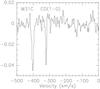 |
Fig. A.1 Signal detected in 2000 at the J2000 coordinates RA 00:43:18.5 Dec +41:17:06, in the OFF signal of position switch observations of M 31C. This spectrum, corresponding to an exposure time of 80 min, was reduced to a 24′′ beam. The y axis displays antenna temperature |

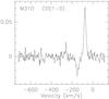 |
Fig. A.2 Signal detected in the OFF positions of M 31D observations, with the wobbler switch observing mode, in 1999 (wobbler throw: 157′′ − 165′′). The y axis displays antenna temperature |
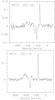 |
Fig. A.3 Signal detected in the OFF positions of M 31G observations, with the wobbler switch observing mode, in 1999 (top: wobbler throw 75′′ − 90′′) and in 2000 (bottom: wobbler throw 94′′ − 104′′). The 2000 observations (bottom panel) was reduced to a 24′′ beam. The y axis displays antenna temperature |
We provide here a short description of the CO signal detected in the OFF positions of the IRAM observations presented in this paper. Their interpretation is beyond the scope of this paper, because they explore a larger area than the ON positions and are only partial.
OFF position of M 31C (position switch)
A clear signal was detected at V0 = −402.3 km s-1 (σ = 12.5 km s-1, ICO = 0.85 K km s-1) and V0 = −320 km s-1 (σ = 5.7 km s-1, ICO = 0.36 K km s-1) in the OFF position of the position switch observations of M 31C, as displayed in Fig. A.1.
OFF position of M 31D (wobbler switch)
For M 31D no OFF signal was detected in the position switch scans performed at the OFF position 122′′, 321′′. However, there is a detectable OFF signal for the scans obtained in wobbler switch mode in 1999, as displayed in Fig. A.2. This signal corresponds to a wobbler throw centred with 157′′ and 165′′ from the ON position. Because the observing procedure was designed to avoid extincted areas and the area surrounding M 31D was not crowded, we suspect that this OFF signal close in velocity to the ON signal is caused by gas on the back side (not detected in extinction). However, complementary observations are required to confirm this hypothesis. The detected signal is at V0 = −147.7 km s-1 (σ = 31.42 km s-1, ICO = 1.12 K km s-1) with an exposure time of 162 min.
OFF position of M 31G (wobbler switch)
No OFF signal was detected in the position switch scans observed for M 31G in 2000 and only wobbler mode has been used in 1999. However, a signal was observed in the OFF positions obtained with the wobbler switch mode, as displayed in Fig. A.3. The throw positions were different in 1999 and 2000 and the OFF signal detected was also different. In 1999 the detected signals are at V0 = −204.5 km s-1 (σ = 17.5 km s-1, ICO = 2.07 K km s-1) and V0 = −242.6 km s-1 (σ = 23.2 km s-1, ICO = 1.42 K km s-1) corresponding to an exposure time of 180 min. In 2000 the OFF signal is detected at V0 = −303.3 km s-1 (σ = 17.6 km s-1, ICO = 1.36 K km s-1), corresponding to an exposure time of 142 min. As discussed in the paper, these OFF positions superimpose on a wide ON signal. Because we do not know the position of the wobble throw (only its distance from the ON position), we can only argue that these OFF signals detected within 1.8 arcmin from the ON position can be associated to the same structure.
Appendix B: HI spectra
Figure B.1 displays the HI velocities obtained for the different positions observed in CO. The positions M 31I and M 31J exhibit one possible component compatible with the disc component detected in CO. There is no clear HI counter-part for the ring component.
All Tables
Characteristics of the CO lines. CO(2 − 1) (resp. CO(2 − 1)) spectra are reduced to a 2.6 kms-1 (resp. 3.2 kms-1) resolution.
AB extinction derived from the map based on the Ciardullo et al. (1988) data as obtained in Melchior et al. (2000).
All Figures
|
Fig. 1 Right: positions (J2000) observed in CO in the central part of M 31.
The circles indicate 1-mm (green) and 3-mm (red) beams of the 10 positions observed
superimposed on the AB extinction map
obtained in Melchior et al. (2000). As
discussed in this paper, the extinction with the central 2 arcsec is not well-defined
on this map. The (blue) cross indicates the centre of M 31 ( |
| In the text | |
|
Fig. 2 Small maps performed at in CO(2 − 1) (left panels) and CO(1−0) (right panels) for the positions A, D and G. The green (resp. red) circles correspond to the FWHM of the CO(2−1) (resp. CO(1−0)) beams at the various positions observed. The corresponding offsets are: (0, 0), (+5, 0), (+2, +4) (−2, +4), (−5, 0), (−2, −4), (+2, −4). The spectra are superimposed on the corresponding AB maps. They are positioned arbitrarily close to the beam corresponding to the observations. |
| In the text | |
|
Fig. 3 Spectra with a detected signal. M 31A, M 31D and M 31G (resp. M 31E, M 31F, M 31I and M 31J) spectra are reduced to a 24″ beam (resp. with the original beam) in CO(2 − 1) and CO(1 − 0). The y-axis provides the antenna temperature in K. |
| In the text | |
|
Fig. 4 Superimposition of the G, I, and J spectra at the nominal spatial resolution, namely 21″ for CO(1−0) and 11″ for CO(2−1). The y-axis provides the antenna temperature in K. |
| In the text | |
|
Fig. 5 Hα+[NII] (left) and [NII] (right) intensities from Ciardullo et al. (1988) and Boulesteix et al. (1987) are displayed with an arbitrary normalisation in the top panels. The bottom left panel presents the CO velocities measured in this paper, superimposed on the gas kinematics based on (1) Hβ and [Oiii] lines measured in slits by Saglia et al. (2010), (2) [Oii] and [Neiii] measured in slits by Ciardullo et al. (1988) and (3) Hα and [Nii] measured in slits by Rubin & Ford (1971). The bottom right panel displays the velocity field obtained with [Nii] λ6584 Ȧ observations (cf. top right panel) based on a Fabry-Perot device by Boulesteix et al. (1987). On each panel, the positions of our CO observations are indicated with circles corresponding to the beams. |
| In the text | |
|
Fig. 6 6.7′ × 6.7′ ionised gas velocity field centred on M 31. Superimposition of the various gas velocities (see Fig. 5 bottom left) on the Boulesteix et al. (1987) Fabry-Perot-derived velocity map. |
| In the text | |
|
Fig. 7 40′′ × 40′′ ionised gas velocity field centred on M 31. Line splittings detected in [Oiii] 5007 Ȧ are superimposed on the velocity field measured on ionised gas by Saglia et al. (2010) and by del Burgo et al. (2000). This velocity field is quite unexpected and do not display any clear rotation pattern. |
| In the text | |
|
Fig. 8 Superposition of the various gas velocities (see Fig. 5 bottom left) (left:) on a simple model of a galactic disc with an inclination of 45 deg, a position angle of 40 deg and a systemic velocity of − 310 kms-1; (right:) similar disc with variable position angles. |
| In the text | |
|
Fig. 9 Image of the HI emission in the very centre, avoiding ± 100 km s-1 around the systemic velocity of − 310 km s-1. This cut has been made to subtract the large-scale HI emission seen in projection superposed to the centre, expected near the systemic velocity. The contours are the dust emission from Spitzer-IRAC (8 μm image where a scaled version of the 3.6 μm image has been subtracted to remove the stellar photospheres emission) (Block et al. 2006). The HI cube is from Braun et al (2009). |
| In the text | |
|
Fig. 10 Velocity field of the HI emission, corresponding to Fig. 9, avoiding large-scale HI emission. |
| In the text | |
|
Fig. 11 Left: superposition of the Hα+ [Nii] map (upper left panel of Fig. 5) of Ciardullo et al. (1988) on the Chandra soft X-ray emission from Bogdán & Gilfanov (2008, see their Fig. 7). The Hα+ [Nii] map has been smoothed with the same smoothing lengths as those used for the Chandra map (A. Bogdan, priv. comm.). Right: superposition of the AB extinction on the 8 μm Spitzer-IRAC map after subtraction of a scaled version of the 3.6 μm image(Block et al. 2006). The AB contours are fixed to 0.05 (blue) and 0.15 (white). |
| In the text | |
|
Fig. 12 Mean density of CO emission from the homogeneous nuclear disc plus tilted ring of the model. The field of view is 200 arcsec in radius, or 0.76 kpc in radius. The density scale, indicated in the wedge, is in arbitrary units. The positions of our CO observations are indicated with circles corresponding to the beams. |
| In the text | |
|
Fig. 13 Density-weighted mean velocity (first moment) of the simulated nuclear region in the same field of view as Fig. 12. Signatures of the tilted ring can be seen at the boarder of the field. The wedge gives the velocity scale inkms-1. |
| In the text | |
|
Fig. 14 Density-weighted velocity dispersion (second moment of the simulated velocity field). The wedge gives the velocity scale in kms-1. The locations of double components with counter-rotating features correspond to the blue and purple regions. |
| In the text | |
|
Fig. 15 Spectra extracted from the simulated cube at the (RA, Dec) offset in arcseconds indicated in each panel. The vertical scale is in arbitrary units. The velocities are centred at the systemic velocity. These offsets correspond the M 31G and M 31I positions. The clumpiness of the gas (not included in the modelling proposed here) is expected to modulate the relative intensity of the various components additionally. |
| In the text | |
|
Fig. 16 Schematic view of the interpretation proposed for the CO velocities observed. The inner disc is presented with a PA of 70 deg and an inclination of 43 deg. The inner ring is superimposed with a similar inclination but a position angle of −35 deg. The straight line indicates the position of the major axis of the main disc inclined by 77 deg with a PA of 35 deg. The bars labelled “N” and “E” have a length of 150 pc. The near (resp. far) sides of the two components are coloured (resp. kept white). The red (resp. blue) colours correspond to the redshift (resp. blueshift) relative to the systemic velocity. |
| In the text | |
|
Fig. B.1 HI spectra obtained with a 1 arcmin resolution for the CO positions discussed in this paper. In each spectrum the velocity of the CO emission is indicated in red. |
| In the text | |
|
Fig. A.1 Signal detected in 2000 at the J2000 coordinates RA 00:43:18.5 Dec +41:17:06, in the OFF signal of position switch observations of M 31C. This spectrum, corresponding to an exposure time of 80 min, was reduced to a 24′′ beam. The y axis displays antenna temperature |
| In the text | |
|
Fig. A.2 Signal detected in the OFF positions of M 31D observations, with the wobbler switch observing mode, in 1999 (wobbler throw: 157′′ − 165′′). The y axis displays antenna temperature |
| In the text | |
|
Fig. A.3 Signal detected in the OFF positions of M 31G observations, with the wobbler switch observing mode, in 1999 (top: wobbler throw 75′′ − 90′′) and in 2000 (bottom: wobbler throw 94′′ − 104′′). The 2000 observations (bottom panel) was reduced to a 24′′ beam. The y axis displays antenna temperature |
| In the text | |
Current usage metrics show cumulative count of Article Views (full-text article views including HTML views, PDF and ePub downloads, according to the available data) and Abstracts Views on Vision4Press platform.
Data correspond to usage on the plateform after 2015. The current usage metrics is available 48-96 hours after online publication and is updated daily on week days.
Initial download of the metrics may take a while.