| Issue |
A&A
Volume 535, November 2011
|
|
|---|---|---|
| Article Number | A123 | |
| Number of page(s) | 8 | |
| Section | The Sun | |
| DOI | https://doi.org/10.1051/0004-6361/200911924 | |
| Published online | 23 November 2011 | |
High time resolution observations of solar Hα flares
II. Search for signatures of electron beam heating
1 Astronomical Institute of Wrocław University, 51-622 Wrocław, ul. Kopernika 11, Poland
e-mail: [radziszewski;rudawy]@astro.uni.wroc.pl
2
Mullard Space Science Laboratory, Holmbury St Mary, Dorking, Surrey RH5 6NT, UK
e-mail: kjhp@mssl.ucl.ac.uk
Received: 23 February 2009
Accepted: 13 September 2011
Aims. The Hα emission of solar flare kernels and associated hard X-ray (HXR) emission often show similar time variations but their light curves are shifted in time by energy transfer mechanisms. We searched for fast radiative response of the chromosphere in the Hα line as a signature of electron beam heating.
Methods. We investigate the time differences with sub-second resolution between the Hα line emission observed with a Multi-channel Subtractive Double Pass (MSDP) spectrograph on the Large Coronagraph and Horizontal Telescope at Białków Observatory, Poland, and HXR emission recorded by the RHESSI spacecraft during several flares, greatly extending our earlier analysis (Paper I) to flares between 2003 and 2005.
Results. For 16 Hα flaring kernels, observed in 12 solar flares, we made 72 measurements of time delays between local maxima of the RHESSI X-ray and Hα emissions. For most kernels, there is an excellent correlation between time variations in the Hα line emission (at line centre and in the line wings) and HXR (20–50 keV) flux, with the Hα emission following features in the HXR light curves generally by a short time lapse Δt = 1–2 s, sometimes significantly longer (10–18 s). We also found a strong spatial correlation.
Conclusions. Owing to our larger number of time measurements than in previous studies, the distribution of Δt values shows a much clearer pattern, with many examples of short (1–2 s) delays of the Hα emission, but with some flares showing longer (10–18 s) delays. The former are consistent with energy transfer along the flaring loop legs by non-thermal electron beams, the latter to the passage of conduction fronts.
Key words: Sun: flares / Sun: X-rays, gamma rays / Sun: activity / Sun: chromosphere
© ESO, 2011
1. Introduction
In Radziszewski et al. (2007) (hereafter Paper I), we discussed high time resolution observations of Hα solar flares made at Białkow Observatory, Poland, and in hard X-rays in the 20–50 keV energy range, as observed with the Reuven Ramaty High-Energy Solar Spectroscopic Imager (RHESSI). Our aim was to establish time correlations between features in the Hα and RHESSI light curves in the flare impulsive stage that will help us to distinguish between mechanisms of energy transfer between the flare energy release site in the corona and the source of Hα emission in the chromosphere. These mechanisms are likely to be either in the form of electron beams or conduction fronts from hot plasmas.
Theoretical investigations (Canfield & Gayley 1987) indicate that intense electron beams travelling from the energy release site to the chromosphere would give rise to explosive evaporation in which heated plasma pushes down on the chromosphere, leading to increases in the Hα line emission in the line centre and its red wing after only ~2 s. Similar results were obtained by Heinzel (1991), though he predicts dips before the main rise in emission, both at the Hα line centre and in the wings (Hα ± 1 Å). On the other hand, Smith & Lilliequist (1979) did calculations for a HXR loop-top source that they had assumed to be thermal rather than non-thermal, deducing that conduction fronts moving at approximately the local ion sound speed (~200 km s-1) would move towards the chromosphere, so enhancing the Hα emission. The travel time for such a conduction front with a typical loop size of a few thousand km would be about 10 s or more.
Flares analysed in this paper.
Observations in Hα have been made over the flare impulsive stage by Kaempfer & Magun (1983), Kurakawa & Takakura (1988), Trottet et al. (2000), Wang et al. (2000), and Kasparova et al. (2005). These observations were made of single flares either over the entire Hα line profile or at specific wavelengths (e.g. at Hα − 1.0 Å in the case of Kurakawa & Takakura 1988). Observations by Hanaoka et al. (2004) and Graeter (1990) at three positions across the Hα profile, including the line centre, were made with time resolutions ranging from 0.033 s to 1.4 s. A comparison of the Hα light curves with emission in either hard X-rays or microwave radio emission in many of these investigations leads to values of Δt (delays in the Hα emission compared with either HXR or microwave radio emission) of between a fraction of a second and several seconds. Our own observations reported in Paper I found that the Hα emission is delayed with respect to HXR observed by RHESSI by 2–3 s for two flares, and up to 17 s for a third.
For a more systematic study of the delay times, many more high time resolution Hα flare observations with simultaneous HXR observations are needed. While three flares were discussed in Paper I, in the present paper we include observations of 12 flares containing one or more small bright regions (called here kernels) in their Hα emission, whose GOES X-ray importance ranges from B to X. These observations, made at nine wavelengths across the Hα line profile and with high time resolution (0.04–0.075 s), represent a considerable improvement over previous investigations, most of which discuss single flares with more modest time resolution and wavelength discrimination. They allow us to compare, for the first time, the distribution of delay times of recognizable features in the Hα light curves with those in hard X-ray light curves. From these data, we are able to state much more definitively than hitherto the origin of the Hα emission features.
2. Observational data and data analysis
Our Hα observations were taken with either the Large Coronagraph (LC) or Horizontal Telescope (HT) using both the Multi-channel Subtractive Double Pass (MSDP) spectrograph (Mein 1991; Rompolt et al. 1994) and fast CCD cameras, all instruments and telescopes being located at Białkow Observatory, University of Wrocław, Poland. The CCD cameras form part of the Solar Eclipse Coronal Imaging System (SECIS: Phillips et al. 2000; Rudawy et al. 2004, 2010), used during solar eclipses. Our objective was to compare Hα flare observations with those of the X-ray emission made with RHESSI. Owing to spacecraft night and SAA passages, RHESSI data were available for only selected Hα observations from the full set of high-cadence observations with the MSDP-SECIS instrument of solar flares or chromospheric brightenings over three summer seasons, 2003–2005. This resulted in 12 flares having MSDP-SECIS observations of Hα kernels that displayed brightness variations apparently similar to those in HXRs (investigated in detail here and indicated in bold type in Table 1), though some others were not. Details are given in Table 1, while information about all our Hα observations (including those with no RHESSI data available) are given in Table 3. The numbering scheme of the kernels follows the notation of this table.
 |
Fig. 1 Hα line centre images of the solar flares on 2004 May 3 and 2005 July 12 observed with the LC-MSDP-SECIS or HT-MSDP-SECIS systems at Białków Observatory. The Hα emission sources (Hα kernels) are marked: K9, K10, K19, K20, K25 and K26, while relevant reference quiet-chromosphere regions are labelled Q. The field of view in these images is 325 × 41 arcsec2 (for top panel) and 942 × 119 arcsec2 (for middle and bottom panels), respectively. Main characteristics of all the analysed flares are given in Table 1. |
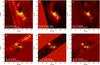 |
Fig. 2 Hα and RHESSI HXR images (reconstructed using the PIXON method, detectors: 3, 4, 5, 6, 8, 9) co-aligned as described in the text. North is towards the top. The RHESSI images are shown as contours (at 50%, 70%, and 90% of maximum of signal). Panels: a), b), c) C8.3 flare – 2005 July 12, 08:00:52–08:00:56 UT (RHESSI 20–50 keV contours), 08:00:54 UT Hα image. Panels: d), e), f) C1.2 flare – 2003 July 16, 16:03:44–16:03:52 UT (RHESSI 12–25 keV contours), 16:03:46 UT Hα image. The dimensions of the areas shown are 128 × 128 arcsec2. |
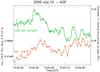 |
Fig. 3 Time variations in the RHESSI HXR (20–50 keV) solar integrated flux (green histogram) and HT-MSDP-SECIS Hα fluxes (red histogram) of the K25 flaring kernel recorded during the M1.0 flare in NOAA 10 786 active region on 2005 July 12. The Hα flux were taken − 0.8 Å from the line centre and are on a linear scale. The RHESSI data are count rates (per second per detector) on a logarithmic scale. The vertical scales indicate the units of each. The integration times are 0.25 s for the demodulated HXR data, and 0.05 s for Hα data. The data were smoothed using a 1-s box-car filter for HXR flux and 0.5-s box-car filter for Hα light curves. The error bars indicate the standard deviations calculated for both light curves. Here and in the next two figures the error bars in the X-ray light curves are plotted on the left, while the error bars of the Hα light curves are plotted on the right. |
The instrumentation has already been described in Paper I so we give only a brief summary here. The MSDP spectrograph has a rectangular entrance window covering an area 325 × 41 arcsec2 on the Sun. A nine-channel prism-box enables data to be collected in the range ± 1.6 Å centred on the Hα line centre, resulting in either quasi-monochromatic images in several wavelengths across the Hα line profile (line centre ± 1.2 Å with a band-width of 0.06 Å for each channel) or complete Hα line profiles for all pixels in the field of view. The images are recorded by one of the two CCD cameras of the SECIS system. The other CCD camera is used to record the precise time from the DCF77 long-wavelength transmitter (the signal of which is generated by a caesium clock). The two SECIS cameras have 512 × 512 pixel2 CCD image sensors (the photometric characteristics of the cameras were discussed by Rudawy et al. 2010) with an image scale ~1 arcsec per pixel. Up to 10 000 images can be taken and stored using a specially adapted computer with proprietary software.
We observed several Hα flares having one or more kernels with time cadences of between 0.04 s (25 images s-1) and 0.075 s (~13 images s-1), depending on the brightness of the observed features. Corrections for small image displacements caused by atmospheric seeing were made by a two-dimensional cross-correlation of well-defined features (e.g. a sunspot visible in far wings of the Hα line), giving a positional accuracy of ~1 pixel. Light curves of the emission of small rectangular areas enclosing each kernel at 13 wavelengths (line centre ± 1.2 Å) across the Hα profile were constructed (see Fig. 1). A small but generally negligible amount of non-flaring chromospheric emission was included in each area. To compensate for brightness changes caused by seeing effects, the flare kernel emission was normalized to the emission observed in a neighbouring region of the quiet chromosphere. These areas are indicated by “Q” in Fig. 1.
Light curves of the flare X-ray emission, generally in the energy range 20–50 keV, were obtained from RHESSI data. (Detectors 1, 3, 4, 5, 6, 7, 8 and 9 were used.) The time resolution of RHESSI is normally determined by the spacecraft spin period (4 s), which is rather too poor for detailed comparison of the flare impulsive stage with the Hα data. However, using a demodulation procedure written by G. Hurford (2004, priv. comm.), the time resolution was improved to 0.25 s. For weaker flares, the RHESSI X-ray emission had poor statistical quality at this demodulation level, thus a box-car smoothing to a 1-s time resolution was applied.
The reality of variations in the Hα emission was established by whether they significantly exceeded the standard deviation in random variations in the amount of emission in the non-flaring areas (marked Q) in Fig. 1. The standard deviations σ are indicated by error bars in the Hα light curves in Figs. 3–5. The uncertainties in the RHESSI light curves are not simply given by those in the count rates assuming Poissonian distributions because of the use of the demodulation technique and (for weaker flares) subsequent smoothing, so we estimated uncertainties in portions of the light curve for each flare showing random variations observed during the pre-flare phase. The combined uncertainties in the RHESSI and Hα emission were then used as a guide to identifications of real features in the light curves. A feature was deemed real if it was at least 3σ above neighbouring emission. Estimations of time lags Δt between the HXR and Hα emission of features were then made by eye. This procedure was found to be a far more sensitive means of evaluating the time differences Δt than using cross-correlation methods. Cross-correlation coefficients r were evaluated, however, as an indication of the degree of similarity between the Hα and RHESSI light curves. These are indicated in Fig. 4.
The connection between the RHESSI and Hα emission for particular events from their relative timings was further confirmed by using RHESSI imaging data for the particular time interval. Data from RHESSI detectors 3, 4, 5, 6, 8, and 9 were used for this, with the PIXON method of image re-construction (Hurford et al. 2002), which is the method that constructs the simplest model of a RHESSI image consistent with the data. The positions of the RHESSI flare emission are obtained in standard solar coordinates, but the precise positions of the Hα emission require the scale and rotation of the Hα images to be determined. This was done by comparing our Hα images with data from the SOHO MDI continuum channel, where sunspots common to both images allow co-alignment to be established and therefore standard solar coordinates of the Hα flare emission with an estimated accuracy of 2 arcsecs. Examples of co-aligned Hα and RHESSI images are shown for two flares in Fig. 2.
3. Results
For 12 flares, we analysed 16 Hα kernels suitable for measuring Δt defined by the time difference between a recognizable local maximum in the Hα light curve (at line centre or the blue or red wings) and the time of a corresponding feature in the RHESSI light curve during the flare impulsive stage. In total, 72 measurements of time delays Δt were made.
We describe the evolution of three flares in particular. All these flares have a wide range of GOES importance, and our results reflect the methods we used to evaluate the Hα delay times Δt. We then discuss the measured delay times for all the analysed flares and the flare number distributions.
3.1. M1 flare of 2005 July 12 (13:02–13:10 UT)
The RHESSI light curve and corresponding Hα light curve of flaring kernel K25 in this M1 flare in NOAA active region 10 768 are shown in Fig. 3. The Hα image of this kernel and K26 is shown in Fig. 1 (bottom panel). The Hα data were taken in the blue wing (−0.8 Å) of the line and are on a linear scale. The integration time was 0.05 s. The RHESSI HXR (20–50 keV) data are photon count rates on a logarithmic scale. We used the Hurford (2004, priv. comm.) demodulation procedure, but as the resulting light curve was somewhat noisy, we applied smoothing with a 1-s box-car filter. This is the light curve shown in Fig. 3.
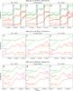 |
Fig. 4 The RHESSI HXR (20–50 keV) and HT-MSDP-SECIS Hα light curves of the K19 and K20 flaring kernels recorded during the C8.3 on 2005 July 12. The Hα light curves are measured at line centre and ± 0.8 Å from the line centre and plotted using a linear scale. The RHESSI data are count rates (per second per detector) on a logarithmic scale. The integration times are 0.25 s for the demodulated HXR data, and 0.05 s for Hα data. The data were smoothed using a 1-s box-car filter for the HXR flux and 0.5-s box-car filter for the Hα light curves. The vertical grey strips in the upper panel (labelled a–f) are magnified in the middle and lower panels of this figure. The error bars indicate the standard deviations calculated for Hα and HXR light curves, except panels b, d, and f where the uncertainties in the HXR curves could not be easily established because of the RHESSI A1 attenuator insertion at 07:59:56 UT. The cross-correlation coefficients r (between HXR and Hα fluxes) are shown in panels a–f. All light curves are normalized to enhance the variations in intensity. The Hα and RHESSI HXR energy flux ranges are defined in Table 2. |
As can be seen in this figure, between 13:03:50 and 13:04:25 UT up to five peaks in the RHESSI (20–50 keV) light curve can be recognized, all with corresponding features in the Hα − 0.8 Å light curve. The Hα peaks have a significance of several standard deviations (indicated in the figure). This allows us to make five separate estimations of Δt, the time that the Hα peak is delayed with respect to the HXR peak, ranging from 1 to 4 s.
3.2. C8.3 flare of 2005 July 12 (07:53–08:10 UT)
For this flare, two bright Hα kernels (K19, K20) exhibited significant time variations that are in some way similar to those in the RHESSI 20–50 keV emission. The light curves of each are shown in Fig. 4, while Fig. 1 (middle panel) shows our measurements for the two regions and the neighbouring emission of active region 10 786 that was to produce the M1 flare discussed in Sect. 3.1 a few hours later.
In the top panel of Fig. 4, the Hα fluxes are for line centre and both wings, ±0.8 Å from the line centre, on a linear scale, while the RHESSI (20–50 keV) data are plotted logarithmically; otherwise the figure is similar to Fig. 3. The time intervals in the vertical grey strips (upper panel, labelled a to f) are shown magnified in the middle and bottom panels. For this flare, the K19 and K20 kernels were observed simultaneously. The brightness of K19 increases in all parts of the Hα profile simultaneously with the HXR (20–50 keV) flux increase, with several statistically significant (>3σ) features present in all light curves. In contrast, the brightness of the K20 kernel in the Hα line blue wing (−0.8 Å from line centre) only starts to increase some 70 seconds after the K19 increase (see Fig. 4, top-left panel). However, the small variations in both the K19 and K20 light curves between 07:59:35 UT and 07:59:52 UT in the Hα blue wing (−0.8 Å) as well as in the red wing (+0.8 Å) were almost simultaneous (Fig. 4, left and right plots of the middle panel). Both of these kernels display very similar variations in the Hα line wings and line centre. During the main increase in the flare (between 08:00:39 UT and 08:00:53 UT), the correlation between the X-ray and Hα light curves measured at the Hα line centre as well as in both wings (at ±0.8 Å) was maintained (see Fig. 4, panels b, d, and f in bottom panel). Almost all the small structures of the HXR (20–50 keV) light curve have corresponding features in the Hα light curves, with very short time delays.
3.3. B2.5 flare of 2004 May 3 (07:24–07:34 UT)
The correlation of the time variations in the HXR integrated flux and Hα light curves for separate flaring kernels are evident even for relatively small flaring events, as in this B2.5 GOES-class solar flare observed on 2004 May 3 (NOAA 10 601). The flare had two clearly separated Hα flaring kernels (K9 and K10, Fig. 1, top panel). However, unlike the C8.3 flare of 2005 July 12, the time variations in the Hα emission of the K9 kernel, in various parts of the line, were different (Fig. 5: Hα light curves at line centre and in both wings at ± 0.6 Å).
During the impulsive stage of the flare (up to 07:25:20 UT), the Hα light curves taken at the line centre and in both the line wings display time variations similar to those of the X-ray (10–20 keV) flux (the increase of HXR emission above 20 keV was too weak to be recorded by RHESSI). Unexpectedly, after 07:25:20 UT the intensities of the Hα light curves taken in both line wings dropped suddenly, roughly to the pre-flare level, and did not reveal any similarities to the X-ray light curve. During the maximum and late phases of the flare, Hα line-centre emission was recorded only, showing a maximum ~20 s after maximum of the X-ray (10–20 keV) emission. This implies that there is a rather slow transport of energy to the chromosphere that is more consistent with the travel time of a conduction front moving at the ion sound speed than electron beam travel times.
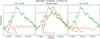 |
Fig. 5 The RHESSI (10–20 keV) and LC-MSDP-SECIS Hα light curves of the K9 flaring kernel during the B2.5 flare on 2004 May 3. The Hα light curves are shown for line centre and ± 0.6 Å from the line centre. The data in the upper panel were smoothed using a 4-s box-car filter for the RHESSI light curve and a 1-s box-car filter for the Hα light curves. The RHESSI light curves in the bottom panel were smoothed using a 0.5-s box-car filter (thin curves) and a 4-s box-car filter (thick curves), while the Hα light curves shown are unsmoothed (thin curves) and smoothed using a 1-s box-car filter (thick curves). The vertical grey strips (labelled a–c) are shown magnified in the bottom panel. The error bars indicate the standard deviations calculated for Hα and X-ray light curves. The Hα and RHESSI HXR energy flux ranges are defined in Table 2. |
The Hα and RHESSI HXR energy flux ranges in Figs. 4 and 5.
Full list of high cadence LC-MSDP-SECIS and HT-MSDP-SECIS Hα observations made in 2003–2005 at the Białków Observatory (Wrocław University, Poland).
3.4. Time delays of Hα features in flares
We selected 12 solar flares observed in MSDP-SECIS Hα and RHESSI HXR (20–50 keV) ranges and investigated 16 kernels, suitable for measurements of the time delays Δt between HXR and Hα local maxima in the light curves. We were able to make 72 measurements of the time delays Δt consisting of 26 measurements for Hα light curves taken in the line centre, 24 measurements for light curves taken in blue wing, and 22 measurements for light curves taken in the red wing.
The histograms of the time delays Δt between HXR (20–50 keV) and Hα local maxima of emission are shown in Fig. 6. The three panels of this figure show relevant time delays between local peaks of: HXR emission and emission measured in the blue wing of the Hα line (panel a), HXR emission and Hα line centre emission (panel b), and HXR emission and emission measured in the red wing of the Hα line (panel c). All histograms show two clearly distinct groups of time delays: many short delays Δt ~ 1–6 s, and a smaller number of features with longer delays, Δt ~ 10–18 s.
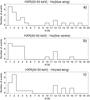 |
Fig. 6 Distribution of all 72 measurements of the time delays Δt between RHESSI HXR (20–50 keV) and MSDP-SECIS Hα localised maxima measured at the line centre a), blue wing b), and red wing c), respectively. |
For all flares with short time delays between HXR and Hα (Δt < 6 s), the cross-correlation coefficients were relatively high, from 0.7 up to 0.9. Over some short time periods for certain flares, such as for the K19 kernel during the impulsive stage of the 2005 July 12 (~08:00 UT) flare, the cross-correlation coefficients were as high as 0.96 (Fig. 4 – panel d).
4. Discussion and conclusions
The histograms of the time-delays show two clearly distinct groups of time delays: many flares have short-time delays Δt ~ 1–6 s, and a few have Δt ~ 10–18 s. The short time delays are consistent with the HXR and Hα source regions being closely separated, with energy transfer by non-thermal electrons from the primary energy source to the chromosphere. The time delays are comparable to those in the model calculations of Heinzel (1991) and Kasparova et al. (2009); however, we did not detect any reduction in Hα emission immediately after the HXR emission as Heinzel (1991) predicts. The longer lasting time delays (10–18 s) may be explained by a slower energy transfer mechanism, perhaps a conduction front moving with the ion sound speed (~200 km s-1) down the flaring loop legs, as discussed in Paper I and by Trottet et al. (2000).
The Hα light curves during the C8.3 solar flare on 2005 July 12 are particularly interesting. Although a brightening in the K20 kernel, which is conspicuous in the Hα blue (0.8 Å) wing, started about 70 s after an increase in the K19 light curve, smaller variations in the K19 and K20 light curves measured in both the blue and red Hα wings (line centre ± 0.8 Å) were similar and almost simultaneous. In addition, the RHESSI 20–50 keV emission was highly correlated with the Hα emission from at least the K19 flaring kernel over the period 08:00:39–08:00:53 UT, having a cross-correlation coefficient of 0.96 (Fig. 4 – panel d). This is consistent with the K19 and K20 kernels being excited simultaneously by non-thermal electron beams travelling down the flaring loop legs if K19 and K20 are the footpoints of the flaring loop, perhaps asymmetrically since the Hα response of the K19 kernel was greater than that of K20. The delayed response of the K20 kernel to the X-ray emission might have been due to chromospheric evaporation at this location (e.g. Falewicz et al. 2009), though in the absence of either X-ray or ultraviolet line profile data we are unable to confirm this.
The time variations of the Hα and X-ray (10–20 keV) light curves recorded during the B2.5 solar flare on 2004 May 3 may be interpreted as energy transfer by electron beams before 07:25:20 UT when the time delays of the Hα variations are very short (Δt < 2 s) relative to the 10–20 keV X-ray emission. These electron beams apparently reach deep into the chromosphere where the Hα line wings are formed. However, after 07:25:20 UT, the Hα line centre light curve appears to be delayed by ~20 s relative to the X-ray, suggesting a more gradual energy transfer, perhaps by conduction which reaches only to the upper chromosphere where the Hα line centre is formed. We note that similar impulsive variations in the soft X-ray emission (at even lower energies, 0.6–3 keV) were recorded by Hudson et al. (1994).
The Hα and RHESSI imaging data illustrates yet more clearly the connection between the chromospheric and X-ray emission; in particular, the images show the very close
correspondence between the hard X-ray and Hα emission for flares that have very small values of Δt.
In summary, the results presented here illustrate how hard X-ray and Hα observations with high time resolution offer much insight into the mechanism whereby energy is transferred from the energy release site in the corona to the chromosphere where the Hα line is formed. The analysis reported here should provide impetus for future observations with fast-frame CCD camera systems on solar telescopes with spectral capabilities such as the system we have been using at Białków Observatory, and the ROSA imaging system currently installed at the National Solar Observatory at Sacramento Peak (Jess et al. 2010).
References
- Canfield, R. C., & Gayley, K. G., 1987, ApJ, 322, 999 [NASA ADS] [CrossRef] [Google Scholar]
- Falewicz, R., Rudawy, P., & Siarkowski, M. 2009, A&A, 508, 971 [NASA ADS] [CrossRef] [EDP Sciences] [Google Scholar]
- Graeter, M. 1990, Sol. Phys., 130, 337 [NASA ADS] [CrossRef] [Google Scholar]
- Hanaoka, Y., Sakurai, T., Noguchi, M., & Ichimoto, K. 2004, Adv. Space Res., 34, 2753 [NASA ADS] [CrossRef] [Google Scholar]
- Heinzel, P. 1991, Sol. Phys., 135, 65 [NASA ADS] [CrossRef] [Google Scholar]
- Hudson, H. S., Strong, K. T., Dennis, B. R., et al. 1994, ApJ, 422, L25 [NASA ADS] [CrossRef] [Google Scholar]
- Hurford, G. J., Schmahl, E. J., Schwartz, R. A., et al. 2002, Sol. Phys., 210, 61 [NASA ADS] [CrossRef] [Google Scholar]
- Jess, D. B., Mathioudakis, M., Christian, D. J., et al. 2010, Sol. Phys., 261, 363 [NASA ADS] [CrossRef] [Google Scholar]
- Kaempfer, N., & Magun, A. 1983, ApJ, 274, 910 [NASA ADS] [CrossRef] [Google Scholar]
- Kasparova, J., Karlicky, M., Kontar, E. P., Schwartz, R. A., & Dennis, B. R. 2005, Sol. Phys., 232, 63 [NASA ADS] [CrossRef] [Google Scholar]
- Kasparova, J., Varady, M., Heinzel, P., Karlicky, M., & Moravec, Z. 2009, A&A, 499, 923 [NASA ADS] [CrossRef] [EDP Sciences] [Google Scholar]
- Kurakawa, H., & Takakura, T. 1988, PASJ, 40, 357 [NASA ADS] [Google Scholar]
- Mein, P. 1991, A&A, 248, 669 [NASA ADS] [Google Scholar]
- Phillips, K. J. H., Read, P. D., Gallagher, P. T., et al. 2000, Sol. Phys., 193, 259 [NASA ADS] [CrossRef] [Google Scholar]
- Radziszewski, K., Rudawy, P., & Phillips, K. J. H. 2007, A&A, 461, 303 (Paper I) [NASA ADS] [CrossRef] [EDP Sciences] [Google Scholar]
- Rompolt, B., Mein, P., Mein, N., et al. 1994, in JOSO Annual Report, ed. A. V. Alvensleben, 87 [Google Scholar]
- Rudawy, P., Phillips, K. J. H., Gallagher, P. T., et al. 2004, A&A, 416, 1179 [NASA ADS] [CrossRef] [EDP Sciences] [Google Scholar]
- Rudawy, P., Phillips, K. J. H., Buczylko, A., Williams, D. R., & Keenan, F. P. 2010, Sol. Phys., 267, 305 [NASA ADS] [CrossRef] [Google Scholar]
- Smith, D. F., & Lilliequist, C. G. 1979, ApJ, 232, 582 [NASA ADS] [CrossRef] [Google Scholar]
- Trottet, G., Rolli, E., Magun, A., et al. 2000, A&A, 356, 1067 [NASA ADS] [Google Scholar]
- Wang, H., Qiu, J., Denker, C., et al. 2000, ApJ, 542, 1080 [NASA ADS] [CrossRef] [Google Scholar]
All Tables
Full list of high cadence LC-MSDP-SECIS and HT-MSDP-SECIS Hα observations made in 2003–2005 at the Białków Observatory (Wrocław University, Poland).
All Figures
|
Fig. 1 Hα line centre images of the solar flares on 2004 May 3 and 2005 July 12 observed with the LC-MSDP-SECIS or HT-MSDP-SECIS systems at Białków Observatory. The Hα emission sources (Hα kernels) are marked: K9, K10, K19, K20, K25 and K26, while relevant reference quiet-chromosphere regions are labelled Q. The field of view in these images is 325 × 41 arcsec2 (for top panel) and 942 × 119 arcsec2 (for middle and bottom panels), respectively. Main characteristics of all the analysed flares are given in Table 1. |
| In the text | |
|
Fig. 2 Hα and RHESSI HXR images (reconstructed using the PIXON method, detectors: 3, 4, 5, 6, 8, 9) co-aligned as described in the text. North is towards the top. The RHESSI images are shown as contours (at 50%, 70%, and 90% of maximum of signal). Panels: a), b), c) C8.3 flare – 2005 July 12, 08:00:52–08:00:56 UT (RHESSI 20–50 keV contours), 08:00:54 UT Hα image. Panels: d), e), f) C1.2 flare – 2003 July 16, 16:03:44–16:03:52 UT (RHESSI 12–25 keV contours), 16:03:46 UT Hα image. The dimensions of the areas shown are 128 × 128 arcsec2. |
| In the text | |
|
Fig. 3 Time variations in the RHESSI HXR (20–50 keV) solar integrated flux (green histogram) and HT-MSDP-SECIS Hα fluxes (red histogram) of the K25 flaring kernel recorded during the M1.0 flare in NOAA 10 786 active region on 2005 July 12. The Hα flux were taken − 0.8 Å from the line centre and are on a linear scale. The RHESSI data are count rates (per second per detector) on a logarithmic scale. The vertical scales indicate the units of each. The integration times are 0.25 s for the demodulated HXR data, and 0.05 s for Hα data. The data were smoothed using a 1-s box-car filter for HXR flux and 0.5-s box-car filter for Hα light curves. The error bars indicate the standard deviations calculated for both light curves. Here and in the next two figures the error bars in the X-ray light curves are plotted on the left, while the error bars of the Hα light curves are plotted on the right. |
| In the text | |
|
Fig. 4 The RHESSI HXR (20–50 keV) and HT-MSDP-SECIS Hα light curves of the K19 and K20 flaring kernels recorded during the C8.3 on 2005 July 12. The Hα light curves are measured at line centre and ± 0.8 Å from the line centre and plotted using a linear scale. The RHESSI data are count rates (per second per detector) on a logarithmic scale. The integration times are 0.25 s for the demodulated HXR data, and 0.05 s for Hα data. The data were smoothed using a 1-s box-car filter for the HXR flux and 0.5-s box-car filter for the Hα light curves. The vertical grey strips in the upper panel (labelled a–f) are magnified in the middle and lower panels of this figure. The error bars indicate the standard deviations calculated for Hα and HXR light curves, except panels b, d, and f where the uncertainties in the HXR curves could not be easily established because of the RHESSI A1 attenuator insertion at 07:59:56 UT. The cross-correlation coefficients r (between HXR and Hα fluxes) are shown in panels a–f. All light curves are normalized to enhance the variations in intensity. The Hα and RHESSI HXR energy flux ranges are defined in Table 2. |
| In the text | |
|
Fig. 5 The RHESSI (10–20 keV) and LC-MSDP-SECIS Hα light curves of the K9 flaring kernel during the B2.5 flare on 2004 May 3. The Hα light curves are shown for line centre and ± 0.6 Å from the line centre. The data in the upper panel were smoothed using a 4-s box-car filter for the RHESSI light curve and a 1-s box-car filter for the Hα light curves. The RHESSI light curves in the bottom panel were smoothed using a 0.5-s box-car filter (thin curves) and a 4-s box-car filter (thick curves), while the Hα light curves shown are unsmoothed (thin curves) and smoothed using a 1-s box-car filter (thick curves). The vertical grey strips (labelled a–c) are shown magnified in the bottom panel. The error bars indicate the standard deviations calculated for Hα and X-ray light curves. The Hα and RHESSI HXR energy flux ranges are defined in Table 2. |
| In the text | |
|
Fig. 6 Distribution of all 72 measurements of the time delays Δt between RHESSI HXR (20–50 keV) and MSDP-SECIS Hα localised maxima measured at the line centre a), blue wing b), and red wing c), respectively. |
| In the text | |
Current usage metrics show cumulative count of Article Views (full-text article views including HTML views, PDF and ePub downloads, according to the available data) and Abstracts Views on Vision4Press platform.
Data correspond to usage on the plateform after 2015. The current usage metrics is available 48-96 hours after online publication and is updated daily on week days.
Initial download of the metrics may take a while.