| Issue |
A&A
Volume 534, October 2011
|
|
|---|---|---|
| Article Number | A84 | |
| Number of page(s) | 15 | |
| Section | Extragalactic astronomy | |
| DOI | https://doi.org/10.1051/0004-6361/201116765 | |
| Published online | 07 October 2011 | |
A nearby GRB host galaxy: VLT/X-shooter observations of HG 031203⋆
1
Max-Planck-Institut für Radioastronomie, Auf dem Hügel 69, 53121 Bonn, Germany
2
Main Astronomical Observatory, Ukrainian National Academy of Sciences, Zabolotnoho 27, Kyiv 03680, Ukraine
e-mail: guseva@mao.kiev.ua
3
Institut für Astrophysik, Göttingen Universität, Friedrich-Hund-Platz 1, 37077 Göttingen, Germany
Received: 22 February 2011
Accepted: 5 August 2011
Context. Long-duration gamma-ray bursts (LGRBs), which release enormous amounts of energy into the interstellar medium, occur in galaxies of generally low metallicity. For a better understanding of this phenomenon, detailed observations of the specific properties of the host galaxies (HG) and the environment near the LGRBs are mandatory.
Aims. We aim at a spectroscopic analysis of HG 031203, the host galaxy of a LRGB burst, to obtain its properties. Our results will be compared with those of previous studies and the properties of a sample of luminous compact emission-line galaxies (LCGs) selected from SDSS DR7.
Methods. Based on VLT/X-shooter spectroscopic observations taken from commissioning mode in the wavelength range ~λλ3200–24 000 Å, we use standard direct methods to evaluate physical conditions and element abundances. The resolving power of the instrument also allowed us to trace the kinematics of the ionised gas. Furthermore, we use X-shooter data together with Spitzer observations in the mid-infrared range for testing hidden star formation.
Results. We derive an interstellar oxygen abundance of 12 + log O/H = 8.20 ± 0.03 for HG 031203. The observed fluxes of hydrogen lines correspond to the theoretical recombination values after correction for extinction with a single value C(Hβ) = 1.67. We produce the CLOUDY photoionisation H ii region model that reproduces observed emission-line fluxes of different ions in the optical range. This model also predicts emission-line fluxes in the near-infrared (NIR) and mid-infrared (MIR) ranges that agree well with the observed ones. This implies that the star-forming region observed in the optical range is the only source of ionisation and there is no additional source of ionisation seen in the NIR and MIR ranges that is hidden in the optical range. We find the composite kinematic structure from profiles of the strong emission lines by decomposing them into two Gaussian narrow and broad components. These components correspond to two H ii regions, separated by ~34 km s-1, and have full widths at half maximum (FWHM) ~ 115 and ~270 km s-1, respectively. We find that the heavy element abundances, extinction-corrected Hα luminosity L(Hα) = 7.27 × 1041 erg s-1, stellar mass M∗ = 2.5 × 10⁸ M⊙, star-formation rate SFR(Hα) = 5.74 M⊙ yr-1 and specific star-formation rate SSFR(Hα) = 2.3 × 10⁻⁸ yr-1 of HG 031203 are in the range that is covered by the LCGs. This implies that the LCGs with extreme star-formation that also comprise green pea galaxies as a subclass may harbour GRBs.
Key words: galaxies: ISM / galaxies: abundances / galaxies: fundamental parameters / galaxies: starburst
© ESO, 2011
1. Introduction
GRB 031203 is one of the two closest (z < 0.2) long-duration gamma-ray bursts (LGRB) known apart from the exceptional GRB 980425.
Most soft-spectrum LGRBs are accompanied by massive stellar explosions (the GRB-supernovae (SNe) connection, see van Paradijs 1999; Woosley & Bloom 2006; Soderberg 2006; Hjorth & Bloom 2011). This and other evidence links LGRBs to ongoing star formation and consequently to the most massive stars as possible progenitors of LGRBs and X-ray flares (XRFs) (Bloom et al. 2002; Le Floc’h et al. 2003; Christensen et al. 2004; Fruchter et al. 2006). Wolf-Rayet (WR) spectral features were found in the spectra of several LGRB host galaxies (HGs) (Hammer et al. 2006; Han et al. 2010). Savaglio et al. (2009) present an extensive study of the most extensive sample of HGs to date, encompassing 46 targets. The authors conclude that there is no compelling evidence that HGs are peculiar galaxies and that they are instead similar to normal star-forming galaxies in the local and distant universe. Accordingly, HGs are proposed to be used as tracers of star formation. Spectroscopic studies of HGs give information on LGRB progenitors and on the physical properties of regions hosting LGRBs. Investigations of HGs have been performed for many galaxies (Christensen et al. 2004; Prochaska et al. 2004; Stanek et al. 2006; Sollerman et al. 2005; Wiersema et al. 2007; Margutti et al. 2007; Thöne et al. 2007; Hammer et al. 2006; Kewley et al. 2007; Thöne et al. 2008; Christensen et al. 2008; Savaglio et al. 2009; Han et al. 2010; Svensson et al. 2010; Watson et al. 2010; Levesque et al. 2010a,b, 2011; Schady et al. 2010; Vergani et al. 2011; Wiersema 2011). However, to date spatially resolved studies have been performed only for several low-redshift HGs (Hammer et al. 2006; Thöne et al. 2008; Christensen et al. 2008; Sollerman et al. 2005; Levesque et al. 2011). For more distant emission-line galaxies at redshifts z ≳ 0.1, the properties of the LGRB environment can be retrieved only from the interstellar medium (ISM) of the entire galaxy, as is the case for HG 031203.
Svensson et al. (2010), Levesque et al. (2010a), Savaglio et al. (2009), Kewley et al. (2007) and Wiersema et al. (2007) found that HGs are relatively low-mass galaxies with a low-metallicity ISM and intense star formation. For a given mass (or luminosity) HGs are systematically offset towards lower metallicities in luminosity-metallicity (L − Z) (Margutti et al. 2007; Stanek et al. 2006; Kewley et al. 2007; Levesque et al. 2010a) or mass-metallicity (M − Z) (Savaglio et al. 2009; Svensson et al. 2010; Levesque et al. 2010b; Vergani et al. 2011) relations as compared to dwarf irregulars and normal star-forming emission-line galaxies (Lequeux et al. 1979; Skillman et al. 1989; Richer & McCall 1995; Kobulnicky & Zaritsky 1999; Melbourne & Salzer 2002; Lee et al. 2004; Pilyugin et al. 2004; Kong 2004; Shi et al. 2005; Lee et al. 2006). Moreover, Levesque et al. (2010b) obtained the offset between nearby HGs with z < 0.3 and nearby SDSS star-forming galaxies as well as between HGs with intermediate-redshift (0.3 < z < 1) and emission-line galaxies from the DEEP2 survey ( ⟨ z ⟩ = 0.8). It was also established that LGRB HGs have lower metallicities than SN HGs without accompanying LGRBs (Fruchter et al. 2006; Modjaz et al. 2008; Levesque et al. 2010a). Kobulnicky (2003) and Savaglio et al. (2005) have found a temporal evolution of emission-line galaxies in L − Z and M − Z diagrams, respectively. Higher redshift galaxies are more metal-poor at a fixed mass or luminosity than local emission-line galaxies. Host galaxies (HGs) are characterised by high star-formation rates (SFRs) and high specific star-formation rates (SSFRs) (Savaglio et al. 2009; Svensson et al. 2010; Levesque et al. 2010a,b).
The metallicities of most HGs are obtained using empirical strong-line methods, such as R23, O3N2, mass-metallicity relation and other calibrations (Savaglio et al. 2005, 2009; Levesque et al. 2010a,b; Svensson et al. 2010; Vergani et al. 2011) and are somewhat uncertain. This is because of a well-known offset between the metallicity obtained by the direct Te-method and empirical strong-line methods. Oxygen abundances obtained by empirical methods are by ~ 0.2–0.6 dex higher than those obtained with the Te-method (Guseva et al. 2009; Hoyos et al. 2005; Shi et al. 2005). Moreover, the luminosity-metallicity relation is also blurred because the metallicity determinations of various galaxy samples do not employ a unique technique. Therefore, we use only a comparison sample of HGs for which the metallicity is derived using the Te-method.
The metallicity of the ISM in the region around the LGRB site may be different from that averaged over the whole galaxy. However, oxygen abundance variations over dwarf compact galaxies are small (~0.1 dex), that is, in the range of errors of abundance determinations (see, e.g. Papaderos et al. 2006; Izotov et al. 2006b). Therefore, the average metallicity of the dwarf HG is comparable to that of the LGRB environment. Thus, in low-mass galaxies the metallicity of an entire galaxy can be a proxy of an LGRB environment.
Therefore, a comprehensive study of HGs that exhibit bright H ii region features is essential for a better understanding of LGRBs and needs to investigate the physical conditions, chemical abundances, extinction, and kinematic structure of their environment.
The long-duration (~30 s) GRB 031203 was discovered in 2003 with INTEGRAL (Götz et al. 2003). A compact dwarf galaxy coinciding with the X-ray source (Hsia et al. 2003) was later identified as the GRB host HG 031203 at redshift z = 0.1055 (Prochaska et al. 2004). Monitoring of the galaxy to search for SNe events led to the discovery of SN2003lw (Tagliaferri et al. 2004). The proximity of the galaxy (it is one of the closest known long-duration GRB host galaxies) allows us to perform a detailed analysis of its properties.
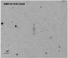 |
Fig. 1 X-shooter acquisition image of HG 031203 [ESO program 60.A-9442(A)] showing the slit location. The galaxy has a compact, slightly elongated shape and likely consists of two H ii regions. North is up and East is to the left. |
An oxygen abundance 12 + log O/H = 7.96 (Te-method) and high reddening E(B − V) = 1.17 corresponding to C(Hβ) = 1.72 were obtained by Levesque et al. (2010a) from Keck I LRIS observations. Based on optical VLT spectra Margutti et al. (2007) derived an oxygen abundance 12 + log O/H = 8.12 ± 0.04. Prochaska et al. (2004) from Magellan/IMACS optical spectroscopy obtained an oxygen abundance 12 + log O/H = 8.02 ± 0.15. This galaxy is located at low galactic latitude, therefore the extinction by the Milky Way is high. Special attention is needed to derive background and intrinsic extinction in HG 031203, which can affect the abundance determination. Margutti et al. (2007) and Prochaska et al. (2004) analysed both the Milky Way and the intrinsic extinction in HG 031203 and derived intrinsic extinction coefficients C(Hβ) = 0.59 and C(Hβ) = 0.46, respectively. Their intrinsic host-galaxy extinctions seem higher that usually obtained in star-forming compact dwarf galaxies. This is mainly because the authors assumed a lower value of the Galactic reddening than that given by Schlegel et al. (1998). On the other hand, the available literature data show no evidence for substantial extinction in any comprehensively studied HGs (Sollerman et al. 2005; Savaglio et al. 2009). Nine out of eleven well-studied GRB HGs collected by Savaglio et al. (2009) have A(V) in the range ~0–0.6 [or C(Hβ) ~ 0–0.3] as derived from the Balmer decrement. For HG 030329 and HG 980425 Sollerman et al. (2005) derived C(Hβ)HG of 0.06 and 0.10, respectively. Therefore, it is likely that Margutti et al. (2007) and Prochaska et al. (2004) overestimated the intrinsic reddening in HG 031203.
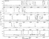 |
Fig. 2 Flux-calibrated VLT/X-shooter near-UV and optical range (UVB + VIS arms) spectrum of the GRB 031203 host galaxy corrected for a redshift of z = 0.1055 (upper spectrum in each panel). The lower spectrum is the upper spectrum downscaled by a factor of 100. The scale of the ordinate is that of the upper spectrum. |
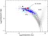 |
Fig. 4 Baldwin-Phillips-Terlevich (BPT) diagram (Baldwin et al. 1981) for luminous compact galaxies (LCGs) from SDSS DR7 (Izotov et al. 2011a) (small blue circles). HG 031203 (this paper) is shown by a large filled red star. The five low-metallicity AGNs from Izotov & Thuan (2008) and Izotov et al. (2010) are indicated by large filled black circles. Host galaxy (HG) 031203 for any data is shown by a star. Other HGs are denoted as follows (see text for details): Savaglio et al. (2009): filled green squares, Levesque et al. (2010a): filled light blue squares, (Christensen et al. 2008): violet asterisks, Hammer et al. (2006): large green open circles, (Wiersema et al. 2007): filled purple triangle, Han et al. (2010): purple diamonds, Margutti et al. (2007): filled purple star, Prochaska et al. (2004): open blue star, Watson et al. (2010): open yellow star. All HGs with emission line fluxes lower than 2 × 10-17 erg s-1 cm-2 are shown by small symbols. Also, the 100 000 emission-line galaxies from SDSS DR7 selected by Izotov et al. (2011a) are shown by grey dots. The dashed line represents the empirical line of Kauffmann et al. (2003) that separates galaxies dominated either by star formation or by an AGN. The continuous line shows the upper limit for purely star-forming galaxies (SFGs) from Stasińska et al. (2006). (A colour version of this figure is available in the online journal.) |
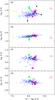 |
Fig. 5 Abundance ratios log N/O a), log Ne/O b), log S/O c) and log Ar/O d) vs. oxygen abundance 12 + log O/H for HG 031203 (this paper) and for LCGs from SDSS DR7 (Izotov et al. 2011a) are shown by large red filled stars and small blue filled circles, respectively. Data from the literature and recalculated from published emission line fluxes are shown by filled and open symbols, respectively. All data for HG 031203 are shown by stars of different colours. Specifically, Margutti et al. (2007): filled and open purple stars, Hammer et al. (2006): filled and open black circles, Wiersema et al. (2007): filled yellow triangles, Levesque et al. (2010a): open light blue squares, Han et al. (2010): open blue rhombs, Prochaska et al. (2004): filled green stars (see text). The solar abundance ratios by Asplund et al. (2009) are indicated by the large purple open circles and the associated error bars. (A colour version of this figure is available in the online journal.) |
We here present high-quality archival VLT/X-shooter spectroscopic observations of HG 031203 over a wide wavelength range, which allows us to derive physical conditions, intrinsic reddening and element abundances in the ionised interstellar medium of the galaxy. The same observations were discussed by Watson et al. (2010). However, they did not draw any conclusions on extinction and heavy element abundances. The observations encompass the near-infrared (NIR) range that allows us to find out whether hidden star formation is present in this galaxy. Such a broad wavelength range extending to the NIR range permits us to derive a more reliable stellar mass (and consequently SSFR) of the galaxy. This is because cool low-mass stars mainly contribute to the stellar mass and they also emit mainly in the NIR range. We note, however, that in low-metallicity compact dwarf galaxies with high SFR the presence of strong ionised gaseous emission complicates the stellar mass determination. We also use the Spitzer observations of Watson et al. (2010) for testing more hidden star formation in the mid-infrared (MIR) range.
The observations are described in Sect. 2. In Sect. 3 we present the main properties of the host galaxy. In particular, the diagnostic diagram is given in Sect. 3.1. The element abundances in HG 031203 are presented in Sect. 3.2. The extinction and hidden star formation are discussed in Sect. 3.3, the CLOUDY modelling and the comparison of the observed and predicted emission-line fluxes in the MIR range are discussed in Sect. 3.4, the kinematic structure in Sect. 3.5, the luminosity-metallicity relation in Sect. 3.6 and the star-formation rate in Sect. 3.7. Our conclusions are summarised in Sect. 4.
2. Observations
A new spectrum of the GRB 031203 host galaxy was obtained during the commissioning of the VLT X-shooter on 2009 March 17 [ESO program 60.A-9024(A)]. In Fig. 1 the acquisition image of HG 031203 with the slit location is shown. The galaxy presents itself as a slightly elongated source with major axis ~1″, which is comparable to the slit width of 0 9–1″. Two H ii regions are present in the galaxy, one brighter than the other. The observations were performed in the wavelength range ~λ3200–24 000 Å at the airmass 1.037 using the three-arm echelle X-shooter spectrograph mounted at the UT2 Cassegrain focus. In the UVB, VIS and NIR arms the total exposure time of 4800 s were broken into four equal subexposures of 1200 s each. Nodding along the slit was performed according to the scheme ABBA with the object positions A or B differing by 5″ along the slit. In the UVB arm with wavelength range λ3233–5600 Å a slit of 1″ × 11″ was used. In the VIS and NIR arms with wavelength ranges λ5475–10 206 Å and λ11 100–23 985 Å, respectively, a slit of 09 × 11″ were used. The binning factor along the spatial and dispersion axes in the UVB and VIS arms was 1, except for the UVB arm where the binning factor along the dispersion axis was 2. The above instrumental set-up resulted in resolving powers λ/Δλ of 10 200, 8800, and 5100 for the UVB, VIS, and NIR arms, respectively. The seeing was ~1″. All observations were obtained at low airmass of ~1.03–1.06, therefore the effect of the atmospheric dispersion is low. The correction for this effect was applied to the UBV and VIS arm spectra during observations. We used the spectrum of the spectrophotometric standard star GD 153 for the flux calibration. The absolute synthetic fluxes for this star were taken from the Space Telescope Science Institute web site1. Spectra of thorium-argon (Th-Ar) comparison arcs were used for wavelength calibration of the UVB and VIS arm observations. For the wavelength calibration of the NIR spectrum we used night-sky emission lines.
In a first step cosmic ray hits of all UVB, VIS, and NIR spectra were removed using the routine CRMEDIAN. The remaining hits were subsequently removed manually after background subtraction. The two-dimensional UVB and VIS spectra were bias-subtracted and flat-field corrected using IRAF2. The two-dimensional NIR spectra were corrected for dark current and divided by the flat frames to correct for the pixel sensitivity variations. For each of the UVB, VIS, and NIR arms we separately coadded spectra with the object at the position A and spectra with the object at the position B. Then, the coadded spectrum at the position B was subtracted from the coadded spectrum at the position A. This resulted in a frame with subtracted background. We used the IRAF software routines IDENTIFY, REIDENTIFY, FITCOORD, and TRANSFORM to perform wavelength calibration and correct for distortion and tilt for each frame. The one-dimensional wavelength-calibrated spectra were then extracted from the two-dimensional frames using the APALL routine. We adopted extraction apertures of 1″ × 25, 09 × 25 and 09 × 25 for the UVB, VIS and NIR spectra, respectively. Before extraction, the spectra at the positions A and B in the two-dimensional background-subtracted frames were carefully aligned with the routine ROTATE and co-added. For the flux calibration we adopted an atmospheric extinction curve for the Cerro Tololo Observatory, which is very similar to that for Cerro Paranal (Patat et al. 2011). Although telluric standards were also observed, no attempts were made to correct for telluric absorption. This is because this correction resulted in very noisy spectra in the regions of strong absorption and does not help much in the determination of the reliable fluxes of the lines that fall in those wavelength ranges. Fortunately, there are many strong lines in regions of low or no telluric absorption. The number of these lines is sufficient for our analysis. In particular, the redshifted strongest NIR emission line Paα is in the region without telluric absorption. The resulting flux-calibrated continuum in all orders is monotonic over the entire range of the spectrum. Therefore, no adjustment of the UVB, VIS, and NIR spectra were needed.
The resulting flux-calibrated and redshift-corrected UVB and VIS spectra of HG 031203 are shown in Fig. 2 and the resulting flux-calibrated and redshift-corrected NIR spectrum is shown in Fig. 3.
3. Results
3.1. Diagnostic diagram
The position of HG 031203 in the [O iii] λ5007/Hβ vs. [N ii] λ6583/Hα Baldwin-Phillips-Terlevich (BPT) diagram (Baldwin et al. 1981) is shown in Fig. 4 by a large filled red star. Luminous compact emission-line galaxies (LCGs) from SDSS DR7 (Izotov et al. 2011a) are shown by small blue circles. The global properties of LCGs are similar to those of the green pea galaxies, which were recently discovered by Cardamone et al. (2009) as a new class of luminous compact galaxies at redshift z ~ 0.1−0.3 with a peculiar bright green colour. Based on the photometrically selected sample of 251 galaxies, Cardamone et al. (2009) found that green pea galaxies have some of the highest specific star-forming rates seen in the local Universe and are similar in size, mass, luminosity, and metallicity to luminous blue compact galaxies and to high-redshift ultraviolet luminous galaxies (Lyman-break galaxies and Ly-α emitters). Izotov et al. (2011a) constructed and studied an extensive sample of 803 star-forming LCGs in a wider redshift range z = 0.02−0.63, selected from SDSS DR7 with the use of spectroscopic and photometric criteria. The five low-metallicity AGN candidates from Izotov & Thuan (2008) and Izotov et al. (2010) are shown by large filled black circles. Data of other authors for HG 031203 are shown by stars in different colours. Other HGs are denoted as follows: Savaglio et al. (2009): filled green squares (031203, 020903 and 060505), Levesque et al. (2010a): filled light blue squares (030329, 020903 and 060218), (Christensen et al. 2008): violet asterisks (980425 – WR, SN regions and entire host galaxy), Hammer et al. (2006): large green open circles (020903 and 980425 (WR and SN regions)), (Wiersema et al. 2007): filled purple triangle (060218), Han et al. (2010): purple diamonds (020903, 030329, 031203, 060218, 060505 GRB site and entire galaxy), Margutti et al. (2007): filled purple star (031203), Prochaska et al. (2004): open blue star (031203), Watson et al. (2010): open yellow star (031203). All HGs with emission line fluxes lower than 2 × 10-17 erg s-1 cm-2 are shown by small symbols. Also, the 100 000 emission-line galaxies from SDSS DR7 are seen as a cloud of grey dots. The dashed line represents the empirical line of Kauffmann et al. (2003), which separates star-forming galaxies and AGNs. The continuous line delineates the upper limit for pure star-forming galaxies from Stasińska et al. (2006).
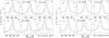 |
Fig. 6 Left panel. Decomposition of strong emission-line profiles into two Gaussian components in the spectrum of HG 031203 for: a) Hβλ4861; b) [O iii] λ4959; c) [O iii] λ5007; d) Hαλ 6563; e) [S iii] λ9532 and f) Paαλ18756. The observed spectrum and the fit are shown by black solid and red dashed lines. The two Gaussian components and residual spectra are shown by blue dashed and black dotted lines. For convenience the observed spectra, Gaussians, and residual are shifted. Right panel. The same as in left panel, but the strong emission line profiles fitted by the single Gaussian. |
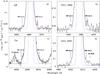 |
Fig. 7 Velocity excess in emission line profiles of a) Hβλ4861; b) [O iii] λ4959; c) Hαλ 6563 and d) [O iii] λ5007. Observational data are shown by solid lines and fits by dotted lines (narrow and broad components of lines in blue and summed fits in red). The positions of the blue-shifted v = 400 km s-1 and red-shifted v = 350 km s-1 broad components are shown by straight lines. |
In Fig. 4 almost all LCGs lie in the low-metallicity part of what is usually considered as the region of star-forming galaxies. HG 031203 is situated on the border between SFG and AGN regions and is close to the region of very low-metallicity AGNs. Photoionisation models of AGN show that lowering their metallicity moves them to the left of BPT diagram, so that they end up in the SFG region (Stasińska et al. 2006). Izotov & Thuan (2008) have concluded that the BPT diagram is unable to distinguish between SFGs and low-metallicity AGNs. The five low-metallicity AGN candidates (Izotov & Thuan 2008; Izotov et al. 2010) also contain the broad components of strong emission lines Hα and Hβ with high luminosities and very steep Balmer decrement. The position of AGN candidates in BPT diagram can be accounted for by the models with the non-thermal radiation contributing less than ~10% to the total radiation (Izotov & Thuan 2008). In particular, the pure photoionisation model without nonthermal radiation agrees quite well with observations (see Sect. 3.4 in this paper). Watson et al. (2010) rule out the presence of an AGN in HG 031203 based on flux ratios of optical emission lines (X-shooter data) and mid-IR spectrum. The authors confirm the previous conclusions of Prochaska et al. (2004) and Margutti et al. (2007). On the other hand, Levesque et al. (2010a), using line-flux ratios from the Keck I LRIS spectrum, concluded that HG 031203 shows evidence of AGN activity.
Overall, HGs including HG 031203 as well as the five low-metallicity candidate AGNs from Izotov & Thuan (2008) and Izotov et al. (2010) lie in the region occupied by LCGs, implying the similarity of their properties. The location of HG 031203 in the upper left region of BPT diagram can be accounted for by the young age of the starburst. Starbursts with older age are instead located in the right lower part of the SFG region.
3.2. Element abundances
Emission-line fluxes
We derived element abundances from emission-line fluxes using a classical semi-empirical method. These lines trace the ISM of HG 031203. The fluxes in all spectra were measured using Gaussian fitting with the IRAF SPLOT routine. The line flux errors include statistical errors derived with SPLOT from non-flux-calibrated spectra, in addition to errors introduced by the absolute flux calibration, which we set to 1% of the line fluxes, according to the uncertainties of absolute fluxes of relatively bright standard stars (Oke 1990; Colina & Bohlin 1994; Bohlin 1996; Izotov & Thuan 2004). These errors will be propagated below into the calculation of the electron temperatures, the electron number densities, and the ionic and total element abundances. Given a function f(x,y,...,z), the uncertainty σ(f) is calculated as  (1)The fluxes were corrected for extinction, using the reddening curve of Cardelli et al. (1989), and for underlying hydrogen stellar absorption (Izotov et al. 1994). The equivalent width of the Hβ emission line is EW(Hβ) = 134 Å corresponding to an age of 3–4 Myr. At this age the predicted equivalent width of the Balmer absorption lines is EW(abs) ~ 2–3 Å (González Delgado et al. 1999; Guseva et al. 2003) with relatively small variations between different hydrogen lines. Therefore we assume that EW(abs) is the same for all hydrogen lines in the same galaxy but varies from galaxy to galaxy. This assumption is justified by the evolutionary stellar population synthesis models of González Delgado et al. (1999, 2005). We also note that 20–30% uncertainties in the EW(abs) for the 3–4 Myr starburst result in <0.2% uncertainties in the fluxes of the strongest emission lines Hβ and Hα, which are most important for the determination of the extinction coefficient. The extinction coefficient C(Hβ) and equivalent widths of the hydrogen absorption lines EW(abs) are calculated simultaneously, which minimises the deviations of corrected fluxes I(λ)/I(Hβ) of all hydrogen Balmer lines from their theoretical recombination values as
  Here f(λ) is the reddening function normalised to the value at the wavelength of the Hβ line, F(λ)/F(Hβ) are the observed hydrogen Balmer emission line fluxes relative to that of Hβ, EW(λ) and EW(Hβ) the equivalent widths of emission lines, and EW(abs) the equivalent widths of hydrogen absorption lines. The extinction-corrected fluxes of emission lines other than those of hydrogen are derived from the equation
 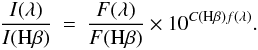 The derived C(Hβ) is applied for correction of all emission-line fluxes in the entire wavelength range λλ3200–24 000 Å.
We varied RV, the ratio of total to selective extinction, in the range from 2.5 to 4.0 and found that these variations change the relative line fluxes by less than ~2%. In the following we adopt RV = 3.2. The extinction-corrected relative fluxes 100 × I(λ)/I(Hβ) of the lines, the extinction coefficient C(Hβ), the equivalent width of the Hβ emission line EW(Hβ), the Hβ observed flux F(Hβ), and the equivalent width of the underlying hydrogen absorption lines EW(abs) are given in Table 1. We note that fluxes of Balmer hydrogen emission lines corrected for extinction and underlying hydrogen absorption (Col. 3 in Table 1) are close to the theoretical recombination values of Hummer & Storey (1987) (Col. 4 of the table), suggesting that the extinction coefficient C(Hβ) is derived reliably.
The physical conditions and the ionic and total heavy element abundances in the ISM of the GRB 031203 host galaxy were derived following Izotov et al. (2006a, Table 2). In particular, we adopt the temperature  (O iii) for O2+, Ne2+, and Ar3+, which is directly derived from the [O iii] λ4363/(λ4959 + λ5007) emission-line ratio. The electron temperatures Te(O ii) and Te(S iii) were derived from the empirical relations by Izotov et al. (2006a) based on a photoionisation model of H ii regions. We also derive (O ii) = (5211 ± 32) K with direct methods based on extinction-corrected fluxes of emission lines from the [O ii]λ(3726+3729)/λ(7320+7330) emission-line ratio, (S iii) = (9488 ± 821) K from the [S iii]λ9069/λ6312 emission-line ratio and (S iii) = (13 282 ± 449) K from the [S iii]λ(9069+9532)/λ6312 emission-line ratio. We used Te(O ii) for the calculation of O+, N+ and S+ abundances and Te(S iii) for the calculation of S2+ and Ar2+ abundances. The electron number densities
  (O ii) = 223 ± 12 and (S ii) = 234 ± 65 were obtained from the [O ii]λ3726/λ3729 and [S ii]λ6717/λ6731 emission-line ratios, respectively. Therefore, the low-density limit holds for the H ii regions that exhibit the narrow line components considered here. Then, the element abundances do not depend sensitively on Ne. The electron temperatures (O iii), Te(O ii), Te(S iii), (S iii) and (O ii), the electron number densities (O ii) and (S ii), the ionisation correction factors (ICFs), and the ionic and total O, N, Ne, S and Ar abundances derived from the forbidden emission lines are given in Table 2.
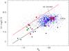 |
Fig. 8 Luminosity-metallicity relation for LCGs from SDSS DR7 (Izotov et al. 2011a) (small blue circles). The location of HG 031203 is shown by the large filled red star. By filled squares are denoted the three most metal-poor BCDs (SBS 0335–052E, SBS 0335–052W and I Zw 18) (Guseva et al. 2009), the intermediate-redshift (z < 1) extremely low-metallicity emission-line galaxies studied by Kakazu et al. (2007), and luminous metal-poor star-forming galaxies at z ~ 0.7 studied by Hoyos et al. (2005). The position of the Lyman-break galaxies at z ~ 3 of Pettini et al. (2001) is marked as LBG with a dotted-line rectangle in the upper right. The emission-line galaxies studied by Guseva et al. (2009) are shown by dots (red dots are data from our observations and black dots are SDSS data). The best linear-likelihood fit to the strongly star-forming galaxies derived by Izotov et al. (2011a) is shown by the black straight line. The fit to emission-line galaxies studied by Guseva et al. (2009) is shown by the red line. Local (z < 0.2) HGs compiled by Margutti et al. (2007) are shown by filled red circles. Data from Levesque et al. (2010a), Hammer et al. (2006) and Han et al. (2010) are shown by green, light blue and purple circles, respectively. (A colour version of this figure is available in the online journal.) |
Physical conditions and element abundances.
Our oxygen abundance of HG 031203 12+logO/H = 8.20 ± 0.03 generally agrees with previous direct determinations of 12 + log O/H in the range ~8.0–8.2 (Prochaska et al. 2004; Hammer et al. 2006; Margutti et al. 2007; Wiersema et al. 2007; Levesque et al. 2010a; Han et al. 2010) (Fig. 5). In particular, the oxygen abundance 12 + logO/H = 8.20 ± 0.03 is consistent with 8.19 estimated by Sollerman et al. (2005) from the thorough analysis presented by Prochaska et al. (2004). On the other hand, our value is slightly higher than the 12 + log O/H = 8.12 ± 0.04 obtained by Margutti et al. (2007) (VLT optical spectra), 8.14 ± 0.07 by Han et al. (2010) and higher than the 12 + log O/H = 8.02 ± 0.15 derived by Prochaska et al. (2004) (Magellan/IMACS optical spectra) and 7.96 derived by Levesque et al. (2010a).
We also recalculated 12 + log O/H with emission-line fluxes given by Margutti et al. (2007), Han et al. (2010), Prochaska et al. (2004) and Levesque et al. (2010a) and obtained 8.22 ± 0.03, 8.15 ± 0.01, 8.06 ± 0.08 and 8.02, respectively, which are higher by ~0.01–0.10 dex that the values in the original papers.
Abundance ratios log N/O, log Ne/O, log S/O and log Ar/O vs. oxygen abundance 12 + log O/H for HG 031203 (this paper) and for LCGs from SDSS DR7 (Izotov et al. 2011a) are shown in Fig. 5 by large red filled stars and small blue filled circles, respectively. We also plot the available abundance ratios from the literature and recalculated values from published emission-line fluxes by filled and open symbols, respectively. Data for HG 031203 are shown by stars of different colours. Specifically, we label data of Margutti et al. (2007) by filled and open purple stars (HG 031203), Hammer et al. (2006) by filled and open black circles (HG 980425, SN and WR regions, HG 020903), Wiersema et al. (2007) by filled yellow triangles (HG 060218), Levesque et al. (2010a) by open light blue squares (HGs 031203, 030329 and 060218), Han et al. (2010) by open blue rhombs (HGs 031203, 030329, 020903 and 060218). Data for HG 031203 from Prochaska et al. (2004) (using solar relative abundances by Grevesse et al. 1996; or by Holweger 2001) are shown by filled green large and small stars, respectively. Abundance ratios obtained by Prochaska et al. (2004), Margutti et al. (2007), Hammer et al. (2006) and our redetermined data obtained from their emission line fluxes are connected by straight lines. The solar abundance ratios by Asplund et al. (2009) are indicated by the large purple open circles and the associated error bars. We use only those data where Te-sensitive [O iii]λ4363 Å emission line is measured.
Wiersema et al. (2007) found the enhanced N/O ratio for several HGs as compared to that in emission-line galaxies. However, our value of log N/O for HG 031203 (Fig. 5a) is lower by 0.3–0.4 dex than log N/O = –0.74 ± 0.20 by Wiersema et al. (2007) and log N/O = –0.83 ± 0.20 by Prochaska et al. (2004), but it is by 0.4 dex higher than log N/O = –1.54 ± 0.08 by Margutti et al. (2007). For HG 060218 Wiersema et al. (2007) obtained log N/O = –1.0 ± 0.4 (our recalculation gives log N/O = –1.19 ± 0.88). As Fig. 5a shows the larger sample of HGs overlaps emission-line galaxies from SDSS DR7. For HG 031203 and HG 060218 and for some emission-line galaxies from SDSS DR7 N/O ratio is higher. This may be owing to local enrichment of the ISM by GRB progenitors or SN remnants.
From the observed spectrum of HG 031203 we derived log Ne/O = –1.15 ± 0.06, using the [Ne iii]λ3868 Å emission line, which is too low compared to the log Ne/O abundance ratio in other emission-line galaxies. This is because the flux ratio [Ne iii]λ3868/λ3967 of 1.13 is very low because the [Ne iii]λ3868Å line is located in a very noisy part of the spectrum which renders its flux uncertain. For comparison, the CLOUDY-predicted line ratio for [Ne iii]I(λ3868)/I(λ3967) is ~3.32 (or F(λ3868)/F(λ3967) ~2.93, if C(Hβ) = 1.67 and the reddening function of Cardelli et al. (1989) are used). Therefore, we use F(3868) = F(3967) × 2.93 for the Ne abundance determination. Then log Ne/O = –0.68 ± 0.05 (see Table 2), which is consistent with the data for LCGs (Izotov et al. 2011a).
Margutti et al. (2007) do not describe how they derived the sulphur abundance. We suspect that their very low sulphur abundance shown in Fig. 5c may have been derived because the [S iii]λ6312 Å emission line was not included for the sulphur abundance determination. To demonstrate this suspicion we show by smaller open symbols in Fig. 5c a sulphur abundance without the [S iii]λ6312 Å emission line. These determinations result in low log S/O ≲ –2.0 and are out of the general relation. Note that our recalculated S/O abundance ratios (in galaxies with detected [S iii]λ6312 Å line (Margutti et al. 2007; and Prochaska et al. 2004, for HG 031203 and Hammer et al. 2006, for HG 980425) are consistent with the S/O determinations for other emission-line galaxies.
Overall, element abundance ratios for a sample of HGs and our log N/O = –1.12 ± 0.04, log Ne/O = –0.68 ± 0.05, log S/O = –1.60 ± 0.05 and log Ar/O = –2.57 ± 0.04 for HG 031203 agree well with the abundance ratios obtained for a large sample of 803 spectra of LCGs (Izotov et al. 2011a).
3.3. Extinction and hidden star formation
That the spectrum of HG 031203 has been obtained simultaneously over the entire optical and near-infrared wavelength ranges eliminates uncertainties introduced by the use of different apertures in the separate optical and NIR observations. In all previous studies of low-metallicity emission-line galaxies except for that of Mrk 59 in Izotov et al. (2009), II Zw 40, Mrk 71, Mrk 996, SBS 0335–052E in Izotov & Thuan (2011) and PHL 293B in Izotov et al. (2011b) the NIR spectra were obtained in separate JHK observations, and there was no wavelength overlap between the optical and NIR spectra. The elimination of these adjusting uncertainties permits us to compare directly the extinctions derived from the optical and NIR spectra.
In the second column of Table 1 we show the observed fluxes F(λ) of the emission lines. The extinction coefficient C(Hβ) and the equivalent width EW(abs) of hydrogen lines are derived from the decrement of hydrogen Balmer lines in the UVB and VIS spectra. The extinction coefficient C(Hβ) = 1.67 is adopted for correction of emission line fluxes in all UVB, VIS, and NIR ranges. In the third column of the same table the corrected fluxes I(λ) are shown. In the fourth column of the table the theoretical recombination fluxes for hydrogen lines calculated by Hummer & Storey (1987) are shown. The relative intensities of hydrogen recombination lines (Hummer & Storey 1987) are calculated for an electron temperature Te = 12 500 K, an electron number density Ne = 100 cm-3, and the case B theory.
Note that the comparison of the observed fluxes of Balmer, Paschen, and Brackett hydrogen lines after correction for extinction with a single value C(Hβ) = 1.67 and the equivalent width EW(abs) of hydrogen lines of 2.0 Å and the theoretical recombination values (Hummer & Storey 1987) shows an agreement within 2–5% for strongest Hδ, Hγ, Hα, and Paα lines. On the other hand, the differences between extinction-corrected and predicted intensities for some lines are high (e.g., for Paβ line) because of the strong telluric absorption. The good agreement implies that a single C(Hβ) can be used over the whole ~λλ3200–24 000 Å range to correct line fluxes for extinction. That the extinction coefficient C(Hβ) does not increase when moving from the optical to the NIR wavelength ranges implies that the NIR emission lines arise in the regions where extinction is not as high and that the NIR emission does not have a hidden star formation compared to the optical emission lines. This appears to be a general result for low-metallicity emission-line galaxies (e.g. Vanzi et al. 2000, 2002; Izotov et al. 2009, 2011b; Izotov & Thuan 2011).
To estimate the intrinsic host-galaxy extinction we used the far-IR map by Schlegel et al. (1998), from which we inferred the reddening value for the Milky Way, EMW(B − V) ≈ 1.037 [or C(Hβ)MW = 1.52]. We derived the estimate of the intrinsic reddening through comparison of C(Hβ)HG = 1.67 derived from Balmer decrement in the spectrum and C(Hβ)MW = 1.52 by Schlegel et al. (1998). Thus, the intrinsic C(Hβ)HG = 0.15 [or A(V)(HG) = 0.33]. This is typical for emission-line dwarf galaxies, but lower than C(Hβ)HG = 0.59 by Margutti et al. (2007) and C(Hβ)HG = 0.46 deduced by Prochaska et al. (2004). Recently Han et al. (2010) obtained C(Hβ)HG = 0.13 ± 0.01. Levesque et al. (2010a) derived the total colour excess in the direction of the galaxy C(Hβ) = 1.72. If the C(Hβ)MW = 1.52 from Schlegel et al. (1998) is adopted, C(Hβ)HG is 0.2. Both these determinations are close to our value of intrinsic extinction.
3.4. CLOUDY stellar photoionisation modelling of the H II region and mid-infrared emission lines
We next examine the excitation mechanisms of all emission lines (not only hydrogen lines) arising in the H ii region of HG 031203. For this purpose, we have constructed stellar photoionisation model for the H ii region using the CLOUDY code (version 07.02.01) of Ferland et al. (1998). We list in Table 3 the input parameters of this model. The first row gives Q(H), the logarithm of the number of ionising photons per second, calculated from the extinction-corrected Hβ luminosity. The other rows of Table 3 list starburst age with the spectral energy distribution of the ionising stellar radiation calculated with Starburst-99 models (Leitherer et al. 1999), and Ne, the electron number density, assumed to be constant with radius. The fourth row gives f, the filling factor. The remaining input parameters are the ratios of number densities of different species to hydrogen, derived from the spectroscopic observations in this paper, except for the carbon abundance. There are no strong emission lines of carbon in the optical and NIR ranges. We therefore calculated its abundance using the mean relation of C/O vs. oxygen abundance derived for low-metallicity H ii regions by Garnett et al. (1995). Parameters Q(H), Ne and chemical composition are derived from the spectra and thus are kept unchanged. The starburst age and filling factor are not constrained by the observational data. Therefore, we varied these two parameters to achieve the best agreement between observations and model predictions. Their adopted values are shown in Table 3.
The CLOUDY-predicted fluxes of the emission lines are shown in the fifth column of Table 1. Comparison of the extinction-corrected observed and predicted emission-line fluxes in both the optical and NIR ranges shows that in general, the agreement between the observations and the CLOUDY predictions is achieved. This implies that a H ii region model including only stellar photoionisation as ionising source is able to account for the observed fluxes both in the optical and NIR ranges. No additional excitation mechanism such as shocks from stellar winds and supernova remnants is needed.
We showed above that the observed emission-line fluxes in the optical and NIR ranges in HG 031203 can be satisfactorily accounted for with the same extinction coefficient C(Hβ) [or the same extinction A(V)]. In other words, there is no more hidden star formation in the NIR range as in the optical range in regions traced by emission lines, i.e. in ionised gas regions. A question then arises: would we see more hidden star formation at longer wavelengths, in the mid-infrared range? To investigate this question in the MIR range, we used the Spitzer observations of Watson et al. (2010). The MIR emission line fluxes relative to the Hβ emission line flux and CLOUDY predicted fluxes are shown in Table 1. No extinction correction was applied to the observed MIR data because it is presumably small in this wavelength range. Comparison of the MIR observed fluxes with those predicted by the pure stellar ionising radiation model shows agreement to within a factor of ~2 or better. The disagreement is the worst for the very weak low-ionisation line [Ne ii] λ12.81 μm, whose flux is predicted to be considerably lower than the observed one.
The agreement between the observed fluxes of the MIR emission-lines and the predicted ones of CLOUDY model, based on the extinction-corrected optical emission lines with C(Hβ) = 1.67, implies that there is only little more hidden star formation seen in the MIR range compared to that in the optical and NIR ranges. This implies that in HG 031203 the MIR emission lines emerge in relatively transparent regions, which are also seen in the optical and NIR ranges. The same conclusion for five other emission-line galaxies were made by Izotov et al. (2009) and Izotov & Thuan (2011).
Input parameters for stellar photoionisation CLOUDY model.
3.5. Kinematic structure
The brightest emission lines in the spectrum of HG 031203 significantly deviate from a single Gaussian line profile (Fig. 6, right panel). We rule out instrumental effects as the cause because no deviations from single Gaussian profiles were detected in night-sky line profiles. To study the kinematic structure of HG 031203 we reassembled all strong emission lines, obtaining narrow and broad components separated by ~ 34 km s-1. Decomposition of Hβ, [O iii] λ4959, λ5007, Hα, [S iii] λ9532 and Paαλ18756 emission line profiles into two Gaussian components is shown in Fig. 6, left panel. The observed spectrum and the fit are shown by black solid and red dashed lines, respectively. Two Gaussian components and residual spectra are shown by blue dashed and black dotted lines, respectively. For convenience the observed spectra, Gaussians, and residuals are shifted along the ordinate axis. Dispersions σres of residual spectra for two cases: 1) fit of observed profile by two Gaussians and 2) fit by single Gaussian, are presented in Table 4. This table and Fig. 6 show that the observed bright emission lines are fitted much better by the two Gaussians.
Dispersions of residual spectra.
In Table 5 we present observed fluxes, FWHM (in km s-1) and F(λ)/F(Hβ) ratios of the narrow and broad components for 14 strong emission lines. The velocity errors are obtained from statistical errors of FWHMs from non-flux-calibrated spectra using the IRAF SPLOT routine.
The FWHMs of the narrow-line components and broad-line components in the spectrum of HG 031203 are ~90–130 km s-1 and ~200–330 km s-1, respectively. The respective average FWHM values for narrow and broad components are ~115 and ~270 km s-1. Note that the Paα profile is likely modified by fringes showing a wavy structure (Fig. 6f). Therefore, the decomposition of the Paα line is not as accurate as that for other lines. The two velocity components of strong emission lines likely arose in two star-forming regions of the host galaxy. HG 031203 is a compact galaxy with a major axis of ~1″, which is comparable to the slit width ~1″. Therefore, it is complicated from its kinematical structure to distinguish between regular rotating disc motion and stochastic motion of H ii regions (e.g. Christensen et al. 2008; Thöne et al. 2008). A similar kinematic structure was found by Wiersema et al. (2007) from two strong emission lines [O iii] λ4959, λ5007 in HG 060218. The authors detected two components separated by ~22 km s-1 that were repeated in Na i and Ca ii absorption lines. The image of AGN candidate Tol 2240–384 (Izotov et al. 2010) also reveals the two H ii regions, separated by ~80 km s-1, if the spectral profiles of strongest emission lines are fitted by two Gaussians.
Observed fluxes of narrow and broad components of strong emission lines.
Parameters of narrow and broad components of strong Balmer lines.
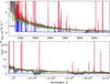 |
Fig. 9 Best-fit model SED to the redshift- and extinction-corrected observed spectrum. The contributions from the stellar and ionised gas components are shown by green and blue lines, respectively. The sum of both stellar and ionised gas emission is shown by the red line. Evidently, the spectrum in the whole wavelength range ~λλ3200–24 000 Å is fitted quite well despite the strong absorption features in the NIR caused by telluric lines. (A colour version of this figure is available in the online journal.) |
In Fig. 7 the velocity excesses in the emission line profiles of Hβλ4861, [O iii] λ4959, Hαλ 6563 and [O iii] λ5007 are shown. Observed profiles are denoted by solid lines and fits by dotted lines. Fits of the narrow and broad components are shown in blue and summed fits in red. The positions of the blue and red velocity excess, corresponding to velocities of v = −400 km s-1 and v = + 350 km s-1, respectively, are shown by vertical tick marks. The bright Paα line is not included in our analysis of the velocity excesses because it could be affected by fringes. This effect is clearly seen in the Paα profile in Fig. 6. Some traces of night-sky absorption lines at the position of Hα (the observed wavelength is 7255 Å) are seen in the blue part of the spectrum (Fig. 7).
We cannot obtain physical conditions and heavy element abundances for the narrow and broad components separately owing to the weakness of the key line [O iii]λ4363. This precludes an accurate separation of narrow and broad components of this line. There is also insufficient spectral resolution for the decomposition of the [O ii]λ3726+3729 emission lines into two pairs of narrow and broad components. An inspection of Table 5 shows that the observed flux ratios F(λ)/F(Hβ) are similar for the broad components and the entire lines but differ from those of the narrow components. Therefore, we calculated the extinction coefficient C(Hβ) of Hγ, Hβ, and Hα for the narrow-component region and obtained C(Hβ) = 1.24 (Table 6). Assuming the same extinction for the region with the broad emission, we obtain a broad Hα/Hβ flux ratio of ~4 or higher than the recombination ratio of ~2.8, suggesting either a higher density of the broad emission region or a higher extinction compared to that in the narrow-line region, or RV different from 3.2. Assuming the higher extinction C(Hβ) = 1.75 for the broad-component region, we obtain robust estimates of the Balmer-line fluxes (Table 6).
3.6. Luminosity-metallicity relation
Since the study by Lequeux et al. (1979) it was established that lower luminosity and lower stellar mass galaxies also have lower metallicities. This conclusion has been confirmed using large samples of galaxies such as those from the SDSS (e.g. Tremonti et al. 2004; Guseva et al. 2009). Nevertheless, some local low-metallicity star-forming galaxies with strong bursts of star formation (e.g. SBS 0335–052E, SBS 0335–052W) and some high-redshift galaxies, such as LBGs, deviate from the luminosity-metallicity (L − Z) relation for the bulk of emission-line galaxies, which are shifted to lower metallicities and/or to higher luminosities (Kunth & Östlin 2000; Guseva et al. 2009; Izotov et al. 2011a).
Adopting B = 22.32 mag from VLT+FORS2 observation of HG 031203 by Margutti et al. (2007) and C(Hβ) = 1.67 we obtain Bcorr = 17.66 mag. At a distance of 430 Mpc taken from the NASA/IPAC Extragalactic Database (NED)3 we derive an absolute magnitude MB = −20.50. The adopted distance was obtained from the radial velocity corrected for Virgo infall with a Hubble constant of 73 km s-1 Mpc-1. For comparison, the absolute blue magnitude MB of HG 031203 from Kewley et al. (2007) is –19.3. Savaglio et al. (2009), who estimated MB in the AB system, found –21.11. We compared the absolute magnitudes MB for HG 031203 with the SDSS g absolute magnitudes Mg for LCGs from Izotov et al. (2011a). This is possible thanks to the prescriptions of Papaderos et al. (2008), who investigated the B − g index and concluded that it is very small and varying in the range of ~0.01–0.03 mag for different star-formation histories of a galaxy.
Figure 8 shows the relation between the oxygen abundance 12 + log O/H and the absolute magnitude Mg in the SDSS g band for the extensive sample of emission-line galaxies studied by Guseva et al. (2009) (red dots for our observations and black dots for SDSS sample) and for LCGs from Izotov et al. (2011a) (small blue circles). The location of HG 031203 with absolute magnitude and oxygen abundance from this paper is denoted by a large red star. The g apparent magnitudes for LCGs and for emission-line galaxies studied by Guseva et al. (2009) are taken from the SDSS. The correction for extinction was made using extinction coefficients C(Hβ) of LCGs derived from Balmer decrement in the SDSS spectra. Distances of LCGs are calculated from redshifts, obtained from strong emission lines. With filled black squares we also show the three most metal-poor BCDs (SBS 0335–052E, SBS 0335–052W and I Zw 18) (Guseva et al. 2009), the intermediate-redshift (z < 1) extremely low-metallicity emission-line galaxies studied by Kakazu et al. (2007) and luminous metal-poor star-forming galaxies at z ~ 0.7 studied by Hoyos et al. (2005). The area occupied by the Lyman-break galaxies at z ~ 3 of Pettini et al. (2001) is denoted as LBG and is displayed as a dotted-line rectangle. The best linear-likelihood fit to the strongly star-forming galaxies derived by Izotov et al. (2011a) is shown in Fig. 8 by a black straight line. The fit to the emission-line galaxies studied by Guseva et al. (2009) is shown by red line. We also show the location of HGs (z < 0.2) compiled by Margutti et al. (2007) by filled red circles (980425, 030329, 031203 and 060218). For HG 030329 and 060218 we used the metallicity obtained from R23 estimates (Table 9 in the paper of Margutti et al. 2007) for which the metallicity calibration of Kewley & Ellison (2008) was applied. Data for HGs 031203, 030329 and 060218 (green circles) are taken from Levesque et al. (2010a); for 020903 (light blue circles) from Hammer et al. (2006), for HGs 990712, 020903, 030329, 031203 and 060218 (purple circles) from Han et al. (2010). Obviously, HG 031203 in the L − M relation is placed in the region of LCGs, which seem to form the bridge between low-mass low-metallicity BCD galaxies with extremely high star-forming activity and high-redshift LBGs (Izotov et al. 2011a).
Thus, HG 031203 is very similar in oxygen abundance and luminosity to LCGs and together with other HGs lies in the region that forms the common luminosity-metallicity relation, obtained by Izotov et al. (2011a) for low-metallicity galaxies with strong star-formation activity. Watson et al. (2010) have concluded that local BCDs (in meaning, low-metallicity galaxies with strong star-formation activity) may be considered as more reliable analogues of star-formation in the early universe than typical local starbursts. Levesque et al. (2010a) also came to conclusion that LGRB host galaxies appear to fall below L − Z relation for local emission-line galaxies, in the region occupied by metal-poor galaxies.
3.7. Star-formation rate
One of the most important characteristics of galaxy evolutionary status is the star-formation rate SFR. We derive the SFR(Hα) using the extinction-corrected luminosity L(Hα) of the Hα emission line and the relation given by Kennicutt (1998), 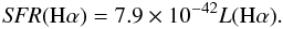 (2)In the equation, the SFR is in units of M⊙ yr-1, L(Hα) in erg s-1, corrected for extinction with C(Hβ) = 1.67 at a distance of 430 Mpc taken from the NED. This results in an extinction-corrected Hα luminosity of 7.27 × 1041 erg s-1. The star-formation rate for HG 031203 is then 5.74 M⊙ yr-1, which is very close to other determinations, for instance, 4.8 M⊙ yr-1, obtained by Levesque et al. (2010a). The star-formation rate for LCGs is in the range 0.7–60 M⊙ yr-1 with an average value of ~4 M⊙ yr-1. Thus, there is no significant difference in the SFR for HG 031203 and average value for LCGs. Along the same line the range of SFRs in LCGs is comparable to that in the intermediate-redshift star-forming galaxies (Hoyos et al. 2005; Kakazu et al. 2007) and in LBGs (Pettini et al. 2001), but is ~10–100 times higher than in typical nearby BCDs. For example, the SFR in I Zw 18 is 0.1 M⊙ yr-1 (Thuan 2008).
The Hβ luminosity of HG 031203 derived from the X-shooter spectrum and corrected for the extinction with C(Hβ) = 1.67 is 2.55 × 1041 erg s-1. Based on the extensive sample of LCGs selected from SDSS DR7, Izotov et al. (2011a) showed that there is a non-redshift-dependent upper limit of L(Hβ) ~ 2.5 × 1042 erg s-1, likely due to a self-regulating mechanism in star formation. All LCGs in Izotov et al. (2011a) range in L(Hβ) from 3 × 1040 to 2.5 × 1042 erg s-1. Thus, L(Hβ) of HG 031203 is in the range of Hβ luminosities of strongly star-forming galaxies.
We derived the stellar mass of HG 031203 by fitting its spectrum with the stellar populations of different ages. This procedure was developed by Guseva et al. (2006, 2007) and Izotov et al. (2011a). We include the ionised gas continuum emission into the fitting procedure because the neglect of this emission in actively star-forming galaxies with EW(Hβ) ≥ 100 Å leads to overestimates of galaxy stellar masses by a factor of several, as was shown in Izotov et al. (2011a).
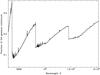 |
Fig. 10 Fraction of gaseous emission to total emission vs. wavelength for the modelled spectrum (EW(Hβ) = 134 Å). The three jumps seen at ~λ3660 Å, ~λ8200 Å and ~λ14 600 Å are caused by the hydrogen Balmer, Paschen, and Brackett discontinuities in the ionised gas emission. |
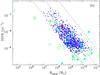 |
Fig. 11 Specific star formation rate SSFR(Hα) vs. the stellar mass M∗ is shown by filled blue circles for LCGs (Izotov et al. 2011a). The location of HG 031203 is marked by the large red star. The dashed lines correspond from left to right to loci with SFR = 1, 10 and 100 M⊙ yr-1, respectively. Data from Svensson et al. (2010) are shown by large green open circles. Open green and purple stars show the position of HG 031203 from Svensson et al. (2010) and Watson et al. (2010), respectively. Data for different HGs from Levesque et al. (2010b) are shown by large filled light-blue squares with HG 031203 shown by a light-blue open star). (A colour version of this figure is available in the online journal.) |
Each fit is performed over the whole observed spectral range ~λλ3200–24 000 Å. The shape of the SED depends on several parameters. Because each SED is the sum of both stellar and ionised gas emission, its shape depends on the relative brightness of stellar and ionised gas emission. In strongly star-forming galaxies, the contribution of the ionised gas can be very high. However, the EWs of hydrogen emission lines never attain the theoretical values for pure ionised gas emission. This implies a non-negligible contribution of stellar emission. We therefore parameterise the relative contribution of gaseous emission to the stellar one by the equivalent width EW(Hβ). The gaseous continuum emission is calculated following Aller (1984) and includes hydrogen and helium free-bound, free-free, and two-photon emission.
The shape of the spectrum also depends on reddening. We have no direct observational constraint for the reddening of the stellar component, which can be different in principle from C(Hβ) obtained from the measured hydrogen line fluxes.
Finally, the SED depends on the star-formation history (SFH) of the galaxy. We carried out a series of Monte Carlo simulations to reproduce the SED. To calculate the contribution of stellar emission to the SEDs, we adopted a grid of the Padua stellar evolution models by Girardi et al. (2000)4 with a heavy element mass fraction Z = 0.004. Using these data we calculated with the package PEGASE.2 (Fioc & Rocca-Volmerange 1997) a grid of instantaneous burst SEDs in a range of ages from 0.5 Myr to 15 Gyr. We adopted a stellar initial mass function with a Salpeter slope, an upper mass limit of 100 M⊙ and a lower mass limit of 0.1 M⊙. Then the SED with any star-formation history can be obtained by integrating the instantaneous burst SEDs over time with a specified time-varying star-formation rate. We approximated the SFH in HG 031203 by a recent short burst, which accounts for the young stellar population, and a continuous star formation responsible for the older stars. The contribution of each type of stellar population to the SED is defined by the ratio of the masses of the old to young stellar populations, b = M(old)/M(young), which we varied between 0.01 and 1000.
Then the total modelled continuum flux near Hβ for a mass of 1 M⊙ is scaled to fit the extinction-corrected luminosity of the galaxy at the same wavelength. The scaling factor is equal to the stellar mass M ∗ of the galaxy.
The flux ratio of the gaseous continuum to the total continuum depends on the adopted electron temperature Te(H+) in the H+ zone, because EW(Hβ) for pure gaseous emission decreases with increasing Te(H+). Given the Te(H+) is not necessarily equal to Te(O iii), we chose to vary it in the range (0.7–1.3)Te(O iii). We assume that the extinction coefficient C(Hβ)stars for the stellar light is the same as C(Hβ)gas for the ionised gas, and vary both in the range (0.8–1.2)C(Hβ), where C(Hβ) is derived from Balmer decrement.
We ran 5 × 10⁵ Monte Carlo models varying simultaneously t(young), t(old), b, Te(H+), C(Hβ)gas and C(Hβ)stars. The best-modelled SED is found from χ2 minimisation of the deviation between the modelled and the observed continuum in ten ranges of the spectrum that are free of the emission lines.
In Fig. 9 we show the best-fit model SED to the redshift- and extinction-corrected spectrum. The contributions from the stellar and ionised gas components are shown by green and blue lines, respectively. The sum of both stellar and ionised gas emission is shown by a red line. The spectrum in the whole range of wavelengths ~λλ3200–24 000 Å is fitted quite well despite the presence of the strong telluric absorption features in the NIR part of the spectrum. Evidently the contribution of gaseous emission is essential because of the EW(Hβ) = 134 Å for the galaxy.
The fraction of the gaseous emission as a function of wavelength in the spectrum of the galaxy is shown in Fig. 10. The three jumps at ~λ3660 Å, ~λ8200 Å and ~λ14 600 Å are caused by the Balmer, Paschen, and Brackett discontinuities of the ionised gas emission. Between these jumps, the fraction of gaseous emission increases with increasing wavelength. As Fig. 10 shows, the fraction of ionised gas continuum-emission in the galaxy with EW(Hβ) = 134 Å increases from <10% to ~25% (in the wavelength range ~4000–8000 Å), from ~14% to ~24% (in the wavelength range ~9000–15 000 Å) and from ~18% to ~26% (in the wavelength range ~15 000–20 000 Å).
The model stellar SED shown in Fig. 9 by the green line is used for the stellar mass (M ∗ ) determination. The mass of HG 031203 is M ∗ = 2.5 × 10⁸ M⊙, which is characteristic for a dwarf galaxy. Then the specific star-formation rate (SSFR) which is defined as SSFR(Hα) = SFR(Hα)/M ∗ for the galaxy, is 2.3 × 10⁻⁸ yr-1. In Fig. 11 the SSFR(Hα) vs. the stellar masses M∗ for LCGs (Izotov et al. 2011a) are shown by filled blue circles. They vary in the range ~10-9–10-7 yr-1. These values are extremely high and similar to those found in high-redshift galaxies at z = 4–6 (Stark et al. 2009) and z = 6–8 (Schaerer & de Barros 2010). The position of HG 031203 is denoted by a large red star. The dashed lines correspond from left to right to loci with SFR = 1, 10 and 100 M⊙ yr-1, respectively. Svensson et al. (2010) obtained the properties (stellar masses, SFRs and SSFRs) for 34 HGs, using a large multi-wavelength (0.45–24 μ) dataset from GOODS and PANS surveys. Data from Svensson et al. (2010) are shown Fig. 11 by large green open circles. Using an unprecedentedly wide wavelength range (~0.3–2 × 105 μm), Watson et al. (2010) have estimated a stellar mass of HG 031203 as log(M∗/M⊙) ~ 9.5. With our estimation of SFR(Hα) we denote the position of HG 031203 in Fig. 11 (using stellar mass of Watson et al. 2010) by open purple star.
There is an offset between the HG sample and LCGs to higher mass (Fig. 11) that can be explained by overestimation of the galaxy’s stellar mass if the ionised gas continuum emission is not included in the fitting of the SED. Several HGs have lower SFRs (those in the left lower part of Fig. 11). In these cases LGRBs arise in ordinary emission-line galaxies with moderate star-formation activity. For comparison, the SFR in the prototype BCD I Zw 18 is much lower, 0.1 M⊙ yr-1 (Thuan 2008).
It is interesting to note that all parameters of the HG 031203 host galaxy and other HGs put them into the class of LCGs. It is reasonable to adopt that many LGRBs occured in the most luminous compact galaxies with low metallicities, because they are characterised by the most vigorous star formation. Overall, we find no appreciable difference in heavy element abundances, elements ratios, luminosities, star-formation rates and specific star-formation rates between HG 031203 and other HGs and LCGs, implying their similar nature.
4. Conclusions
We have studied the spectrum of the GRB 031203 host galaxy (HG 031203) with the VLT/X-shooter spectroscopic observations in the wavelength range ~λλ3200–24 000 Å. These data were compared with the data obtained previously by Izotov et al. (2011a) for luminous compact emission-line galaxies (LCGs) from SDSS DR7. We have arrived at the following conclusions:
-
1.
We derive the oxygen abundance of 12 + logO/H = 8.20 ± 0.03 in the H ii region of HG 031203.The previous direct determinations (Prochaskaet al. 2004; Hammeret al. 2006; Marguttiet al. 2007; Wiersemaet al. 2007; Levesqueet al. 2010a; Hanet al. 2010) give the oxygen abun-dance 12 + log O/H in the range ~8.0–8.2.
-
2.
We find that the extinction-corrected fluxes of hydrogen Balmer, Paschen, and Brackett lines agree well with the theoretical recombination values if a single value of the extinction coefficient C(Hβ) = 1.67 is adopted. This implies that there is no additional star formation that is seen in the NIR range but is hidden in the visible range. The star-forming region observed in the optical range is the only source of ionisation.
-
3.
Using Spitzer MIR emission-line fluxes, we have also found that MIR data do not reveal an additional star formation that is hidden at shorter wavelengths. Thus, the emission-line spectrum of HG 031203 in the whole ~0.36–20 μm wavelength range originates in relatively transparent H ii regions.
-
4.
The profiles of strong emission lines are decomposed into two Gaussian narrow and broad components with FWHM ~ 115 and ~270 km s-1, respectively. These components, separated by ~34 km s-1, likely correspond to two H ii regions with different extinction, which is larger in the region with a broad component.
-
5.
We derive a stellar mass M∗ = 2.5 × 10⁸ M⊙ for HG 031203 by fitting its spectrum with the stellar populations of different ages (Izotov et al. 2011a; Guseva et al. 2006, 2007). We include the ionised gas continuum emission in the fitting procedure because the neglect of this emission in the actively star-forming galaxy with EW(Hβ) = 134 Å leads to an overestimate of the M∗ (Izotov et al. 2011a).
-
6.
We find that the heavy element abundances, element abundance ratios, extinction-corrected Hα luminosity L(Hα) = 7.27 × 1041 erg s-1, star-formation rate SFR(Hα) = 5.74 M⊙ yr-1 and specific star-formation rate SSFR(Hα) = SFR(Hα)/M∗ = 2.3 × 10⁻⁸ yr-1 of HG 031203 and other HGs are in the range occupied by the LCGs from SDSS DR7 studied by Izotov et al. (2011a). In [O iii] λ5007/Hβ vs. [N ii] λ6583/Hα diagnostic diagram (Baldwin et al. 1981) and in the luminosity-metallicity diagram the GRB host galaxy is also placed in the region of the LCGs. This implies that LCGs with extreme star formation (containing also green pea galaxies as a subclass of LCGs Cardamone et al. 2009) may predominantly harbour the long-duration GRBs.
Acknowledgments
N.G.G., Y.I.I. and K.J.F. are grateful to the staff of the Max Planck Institute for Radioastronomy for their warm hospitality and acknowledge support through DFG grant No. FR 325/59-1. This research has made use of the NASA/IPAC Extragalactic Database (NED), which is operated by the Jet Propulsion Laboratory, California Institute of Technology, under contract with the National Aeronautics and Space Administration.
References
- Aller, L. H. 1984, Physics of Thermal Gaseous Nabulae (Dordrecht: Reidel) [Google Scholar]
- Asplund, M., Grevesse, N., Sauval, A. J., & Scott, P. 2009, ARA&A, 47, 481 [NASA ADS] [CrossRef] [Google Scholar]
- Baldwin, J. A., Phillips, M. M., & Terlevich, R. 1981, PASP, 93, 5 [NASA ADS] [CrossRef] [EDP Sciences] [Google Scholar]
- Bloom, J. S., Kulkarni, S. R., & Djorgovski, S. G. 2002, AJ, 123, 1111 [NASA ADS] [CrossRef] [Google Scholar]
- Bohlin, R. C. 1996, AJ, 111, 1743 [NASA ADS] [CrossRef] [Google Scholar]
- Cardamone, C., et al. 2009, MNRAS, 399, 1199 [Google Scholar]
- Cardelli, J. A., Clayton, G. C., & Mathis, J. S. 1989, ApJ, 345, 245 [NASA ADS] [CrossRef] [Google Scholar]
- Chary, R., Becklin, E. E., & Armus, L. 2002, ApJ, 566, 229 [NASA ADS] [CrossRef] [Google Scholar]
- Christensen, L., Hjorth, J., & Gorosabel, J. 2004, A&A, 425, 913 [NASA ADS] [CrossRef] [EDP Sciences] [Google Scholar]
- Christensen, L., Vreeswijk, P. M., Sollerman, J., et al. 2008, A&A, 490, 45 [NASA ADS] [CrossRef] [EDP Sciences] [Google Scholar]
- Colina, L., & Bohlin, R. C. 1994, AJ, 108, 1931 [NASA ADS] [CrossRef] [Google Scholar]
- Fioc, M., & Rocca-Volmerange, B. 1997, A&A, 326, 950 [NASA ADS] [Google Scholar]
- Ferland, G. J., Korista, K. T., Verner, D. A., et al. 1998, PASP, 110, 761 [Google Scholar]
- Fruchter, A. S., Levan, A. J., Strolger, L., et al. 2006, Nature, 441, 463 [NASA ADS] [CrossRef] [PubMed] [Google Scholar]
- Garnett, D. R., Skillman, E. D., Dufour, R. J., et al. 1995, ApJ, 443, 64 [NASA ADS] [CrossRef] [Google Scholar]
- Girardi, L., Bressan, A., Bertelli, G., & Chiosi, C. 2000, A&AS, 141, 371 [Google Scholar]
- González Delgado, R. M., Leitherer, C., Heckman, T. M. 1999, ApJS, 125, 489 [NASA ADS] [CrossRef] [Google Scholar]
- González Delgado, R. M., Cerviño, M., Martins, L. P., Leitherer, C., & Hauschildt, P. H. 2005, MNRAS, 357, 945 [NASA ADS] [CrossRef] [Google Scholar]
- Gorosabel, J., Prez-Ramrez, D., Sollerman, J., et al. 2005, A&A, 444, 711 [NASA ADS] [CrossRef] [EDP Sciences] [Google Scholar]
- Götz, D, Mereghetti, S., Beck, M., & Borkowski, J. 2003, GCN Circ., 2459 [Google Scholar]
- Grevesse, N., Noels, A., & Sauval, A. J. 1996, in Cosmic abundances, ed. S. Holt, & G. Sonneborn (San Fransisco: ASP), ASP Conf. Ser. 99, 117 [Google Scholar]
- Guseva, N. G., Papaderos, P., Izotov, Y. I., et al. 2003, A&A, 407, 91 [NASA ADS] [CrossRef] [EDP Sciences] [Google Scholar]
- Guseva, N. G., Izotov, Y. I., & Thuan, T. X. 2006, ApJ, 644, 890 [NASA ADS] [CrossRef] [Google Scholar]
- Guseva, N. G., Izotov, Y. I., Papaderos, P., & Fricke, K. J. 2007, A&A, 464, 885 [NASA ADS] [CrossRef] [EDP Sciences] [Google Scholar]
- Guseva, N. G., Papaderos, P., Meyer, H. T., Izotov, Y. I., & Fricke, K. J. 2009, A&A, 505, 63 [NASA ADS] [CrossRef] [EDP Sciences] [Google Scholar]
- Hammer, F., Flores, H., Schaerer, D., et al. 2006, A&A, 454, 103 [NASA ADS] [CrossRef] [EDP Sciences] [Google Scholar]
- Han, X. H., Hammer, F., Liang, Y. C. et al 2010, A&A, 514, A24 [NASA ADS] [CrossRef] [EDP Sciences] [Google Scholar]
- Hjorth, J., & Bloom, J. S. 2011, in Gamma-Ray Bursts, eds. C., Kouveliotou, R. A. M. J., Wijers, & S. E. Woosley (Cambridge University Press) [arXiv:1104.2274] [Google Scholar]
- Holland, S. T., Sbarufatti, B., & Shen, R. 2010, ApJ, 717, 223 [NASA ADS] [CrossRef] [Google Scholar]
- Holweger, H. 2001, in Solar and Galactic Composition, ed. R. F. Wimmer-Schweingruber (Melville: AIP), AIP Conf. Proc., 598, 23 [Google Scholar]
- Hoyos, C., Koo, D. C., Phillips, A. C., Willmer, C. N. A., & Guhathakurta, P. 2005, ApJ, 635, L21 [NASA ADS] [CrossRef] [Google Scholar]
- Hsia, C. H., Lin, H. C., Huang, K. Y., Urata, Y., & Tamagawa, T. 2003, GCN Circ., 2470 [Google Scholar]
- Hummer, D. G., & Storey, P. J. 1987, MNRAS, 224, 801 [NASA ADS] [CrossRef] [Google Scholar]
- Izotov, Y. I., & Thuan, T. X. 2004, ApJ, 602, 200 [CrossRef] [Google Scholar]
- Izotov, Y. I., & Thuan, T. X. 2008, ApJ, 687, 133 [NASA ADS] [CrossRef] [Google Scholar]
- Izotov, Y. I., & Thuan, T. X. 2011, ApJ, 734, 82 [NASA ADS] [CrossRef] [Google Scholar]
- Izotov, Y. I., Thuan, T. X., & Lipovetsky, V. A. 1994, ApJ, 435, 647 [NASA ADS] [CrossRef] [Google Scholar]
- Izotov, Y. I., Stasińska, G., Meynet, G., Guseva, N. G., & Thuan, T. X. 2006a, A&A, 448, 955 [NASA ADS] [CrossRef] [EDP Sciences] [Google Scholar]
- Izotov, Y. I., Schaerer, D., Blecha, A., et al. 2006b, A&A, 459, 71 [NASA ADS] [CrossRef] [EDP Sciences] [Google Scholar]
- Izotov, Y. I., Thuan, T. X., & Guseva, N. G. 2007, ApJ, 671, 1297 [NASA ADS] [CrossRef] [Google Scholar]
- Izotov, Y. I., Thuan, T. X., & Wilson, J. C. 2009, ApJ, 703, 1984 [NASA ADS] [CrossRef] [Google Scholar]
- Izotov, Y. I., Guseva, N. G., Fricke, K. J., et al. 2010, A&A, 517, A90 [NASA ADS] [CrossRef] [EDP Sciences] [Google Scholar]
- Izotov, Y. I., Guseva, N. G., & Thuan, T. X. 2011a, ApJ, 728, 161 [NASA ADS] [CrossRef] [Google Scholar]
- Izotov, Y. I., Guseva, N. G., Fricke, K. J., & Henkel, C. 2011b, A&A, 533, A25 [NASA ADS] [CrossRef] [EDP Sciences] [Google Scholar]
- Kakazu, Y., Cowie, L. L., & Hu, E. M. 2007, ApJ, 668, 853 [NASA ADS] [CrossRef] [Google Scholar]
- Kauffmann, G., Heckman, T. M., Tremonti, C., et al. 2003, MNRAS, 346, 1055 [Google Scholar]
- Kennicutt, R. C. Jr. 1998, ARA&A, 36, 189 [Google Scholar]
- Kelly, P. L., Kirshner, R. P., & Pahre, M. 2008, ApJ, 687, 1201 [NASA ADS] [CrossRef] [Google Scholar]
- Kewley, L. J., & Ellison, S. L. 2008, ApJ, 681, 1183 [NASA ADS] [CrossRef] [Google Scholar]
- Kewley, L. J., Brown, W. R.,Geller, M. J., Kenyon, S. J., & Kurtz, M. J. 2007, AJ, 133, 882 [NASA ADS] [CrossRef] [Google Scholar]
- Kobulnicky, H. A. 2003, ApJ, 599, 1006 [NASA ADS] [CrossRef] [Google Scholar]
- Kobulnicky, H. A., & Zaritsky, D. 1999, ApJ, 511, 118 [NASA ADS] [CrossRef] [Google Scholar]
- Kong, X. 2004, A&A, 425, 417 [NASA ADS] [CrossRef] [EDP Sciences] [Google Scholar]
- Kunth, D., & Óstlin, G. 2000, A&AR, 10, 1 [Google Scholar]
- Lee, J. C., Salzer, J. J., & Melbourne, J. 2004, ApJ, 616, 752 [NASA ADS] [CrossRef] [Google Scholar]
- Lee, H., Skillman, E. D., Cannon, J. M., et al. 2006, ApJ, 647, 970 [NASA ADS] [CrossRef] [Google Scholar]
- Le Floc’h, E.,Duc, P.-A., Mirabel, I. F., et al. 2003, A&A, 400, 499 [NASA ADS] [CrossRef] [EDP Sciences] [Google Scholar]
- Leitherer, C., Schaerer, D., Goldader, J. D., et al. 1999, ApJS, 123, 3 [NASA ADS] [CrossRef] [Google Scholar]
- Lequeux, J., Peimbert, M., Rayo, J. F., et al. 1979, A&A, 80, 155 [NASA ADS] [Google Scholar]
- Levesque, E. M., Berger, E., Kewley, L. J., et al. 2010a, AJ, 139, 694 [NASA ADS] [CrossRef] [Google Scholar]
- Levesque, E. M., Kewley, L. J., Berger, E., & Zahid, H. J. 2010b, AJ, 140, 1557 [NASA ADS] [CrossRef] [Google Scholar]
- Levesque, E. M., Berger, E., Soderberg, A. M., & Chornock, R. 2011, ApJ, 739, 23 [NASA ADS] [CrossRef] [Google Scholar]
- Margutti, R., Chincarini, G., Covino, S., et al. 2007, A&A, 474, 815 [NASA ADS] [CrossRef] [EDP Sciences] [Google Scholar]
- Melbourne, J., & Salzer, J. J. 2002, AJ, 123, 2302 [NASA ADS] [CrossRef] [Google Scholar]
- Melbourne, J., Phillips, A., Salzer, J. J., Gronwall, C., & Sarajedini, V. L. 2004, AJ, 127, 686 [NASA ADS] [CrossRef] [Google Scholar]
- Modjaz, M., Kewley, L. J., Kirshner, R. P., et al. 2008, AJ, 135, 1136 [NASA ADS] [CrossRef] [Google Scholar]
- Oke, J. B. 1990, AJ, 99, 1621 [NASA ADS] [CrossRef] [Google Scholar]
- Papaderos, P., Izotov, Y. I., Guseva, N. G., et al. 2006, A&A, 454, 119 [NASA ADS] [CrossRef] [EDP Sciences] [Google Scholar]
- Papaderos, P., Guseva, N. G., Izotov, Y. I., & Fricke, K. J. 2008, A&A, 491, 113 [NASA ADS] [CrossRef] [EDP Sciences] [Google Scholar]
- Patat, F., Moehler, S., O’Brien, K., et al. 2011, A&A, 527, A91 [NASA ADS] [CrossRef] [EDP Sciences] [Google Scholar]
- Pettini, M., Shapley, A. E., Steidel, C. C., et al. 2001, ApJ, 554, 981 [NASA ADS] [CrossRef] [Google Scholar]
- Pilyugin, L. S., Vílchez, J. M., & Contini, T. 2004, A&A, 425, 849 [NASA ADS] [CrossRef] [EDP Sciences] [Google Scholar]
- Piran, T. 2004, Rev. Mod. Phys., 76, 4, 1143 [Google Scholar]
- Prochaska, J. X., Bloom, J., Chen, H.-W., et al. 2004, ApJ, 611, 200 [NASA ADS] [CrossRef] [Google Scholar]
- Richer, M. G., & MacCall, M. L. 1995, ApJ, 445, 642 [NASA ADS] [CrossRef] [Google Scholar]
- Savaglio, S., Glazebrook, K., Borgne, D. Le., et al. 2005, ApJ, 635, 260 [NASA ADS] [CrossRef] [Google Scholar]
- Savaglio, S., Glazebrook, K., & Borgne, D. Le. 2009, ApJ, 691, 182 [NASA ADS] [CrossRef] [MathSciNet] [Google Scholar]
- Schady, P., Page, M. J., Oates, S. R., et al. 2010, MNRAS, 401, 2773 [NASA ADS] [CrossRef] [Google Scholar]
- Schaerer, D., & de Barros, S. 2010, A&A, 515, 73 [Google Scholar]
- Schlegel, D. J., Finkbeiner, D. P., & Davis, M. 1998, ApJ, 500, 525 [NASA ADS] [CrossRef] [Google Scholar]
- Shi, F., Kong, X., Li, C., & Cheng, F. Z. 2005, A&A, 437, 849 [NASA ADS] [CrossRef] [EDP Sciences] [Google Scholar]
- Skillman, E. D., Kennicutt, R. C., Jr., & Hodge, P. W. 1989, ApJ, 347, 875 [NASA ADS] [CrossRef] [Google Scholar]
- Soderberg, A. M. 2006, Proceedings of the 16th Annual October Astrophysics Conference in Maryland Gamma Ray Bursts in the Swift Era, ed. S. Holt, N. Gehrels, & J. Nousek, Conf. Ser., 836, 380 [Google Scholar]
- Sollerman, J., Östlin, G., Fynbo, J. P. U., et al. 2005, New A, 11, 103 [Google Scholar]
- Stanek, K. Z., Garnavich, P. M., Nutzman, P. A., et al. 2005, ApJ, 626, L5 [NASA ADS] [CrossRef] [Google Scholar]
- Stanek, K. Z., Gnedin, O. Y., Beacom, J. F., et al. 2006, Acta Astron., 56, 333 [NASA ADS] [Google Scholar]
- Stark, D. P., Ellis, R. S., Bunker, A., et al. 2009, ApJ, 697, 1493 [NASA ADS] [CrossRef] [Google Scholar]
- Starling, R. L. C., Wiersema, K., Levan, A. J., et al. 2011, MNRAS, 411, 2792 [NASA ADS] [CrossRef] [Google Scholar]
- Stasińska, G., Cid Fernandes, R., Mateus, A., Sodré, L., & Asari, N. V. 2006, MNRAS, 371, 972 [NASA ADS] [CrossRef] [Google Scholar]
- Svensson, K. M., Levan, A. J., Tanvir, N. R., et al. 2010, MNRAS, 405, 57 [NASA ADS] [Google Scholar]
- Tagliaferri, G., Covino, S., Fugazza, D., et al. 2004, IAU Circ., 8308, 1 [NASA ADS] [Google Scholar]
- Thöne, C. C., Greiner, J., Savagloi, S., & Jehin, E. 2007, ApJ, 671, 628 [NASA ADS] [CrossRef] [Google Scholar]
- Thöne, C. C., Fynbo, J. P. U., Östlin, G., et al. 2008, ApJ, 676, 1151 [NASA ADS] [CrossRef] [Google Scholar]
- Thuan, T. X. 2008, in Low-metallicity star formation: from the first stars to dwarf galaxies, ed. L. Hunt, S. C. Madden, & R. Schneider (Cambridge: Cambridge Univ. Press), 348 [Google Scholar]
- Tremonti, C. A., Heckman, T. M., Kauffmann, G., et al. 2004, ApJ, 613, 898 [NASA ADS] [CrossRef] [Google Scholar]
- van Paradijs, J. 1999, Science, 286, 693 [NASA ADS] [CrossRef] [Google Scholar]
- Vanzi, L., Hunt, L. K., Thuan, T. X., & Izotov, Y. I. 2000, A&A, 363, 493 [NASA ADS] [Google Scholar]
- Vanzi, L., Hunt, L. K., & Thuan, T. X. 2002, A&A, 390, 481 [NASA ADS] [CrossRef] [EDP Sciences] [Google Scholar]
- Vergani, S. D., Flores, H., Covino, S., et al. 2011, A&A, accepted [arXiv:1107.3841] [Google Scholar]
- Watson, D., French, J., Christensen, L., et al. 2010, ApJ, submitted [arXiv:1010.1783] [Google Scholar]
- Wiersema, K. 2011, MNRAS, 414, 2793 [NASA ADS] [CrossRef] [Google Scholar]
- Wiersema, K., Savaglio, S., Vreeswijk, P. M., et al. 2007, A&A, 464, 529 [NASA ADS] [CrossRef] [EDP Sciences] [Google Scholar]
- Woosley, S. E. 1993, ApJ, 405, 273 [NASA ADS] [CrossRef] [Google Scholar]
- Woosley, S. E., & Bloom, J. S. 2006, ARA&A, 44, 507 [NASA ADS] [CrossRef] [Google Scholar]
All Tables
All Figures
|
Fig. 1 X-shooter acquisition image of HG 031203 [ESO program 60.A-9442(A)] showing the slit location. The galaxy has a compact, slightly elongated shape and likely consists of two H ii regions. North is up and East is to the left. |
| In the text | |
|
Fig. 2 Flux-calibrated VLT/X-shooter near-UV and optical range (UVB + VIS arms) spectrum of the GRB 031203 host galaxy corrected for a redshift of z = 0.1055 (upper spectrum in each panel). The lower spectrum is the upper spectrum downscaled by a factor of 100. The scale of the ordinate is that of the upper spectrum. |
| In the text | |
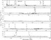 |
Fig. 3 Same as Fig. 2 but for the near-infrared (NIR) range. |
| In the text | |
|
Fig. 4 Baldwin-Phillips-Terlevich (BPT) diagram (Baldwin et al. 1981) for luminous compact galaxies (LCGs) from SDSS DR7 (Izotov et al. 2011a) (small blue circles). HG 031203 (this paper) is shown by a large filled red star. The five low-metallicity AGNs from Izotov & Thuan (2008) and Izotov et al. (2010) are indicated by large filled black circles. Host galaxy (HG) 031203 for any data is shown by a star. Other HGs are denoted as follows (see text for details): Savaglio et al. (2009): filled green squares, Levesque et al. (2010a): filled light blue squares, (Christensen et al. 2008): violet asterisks, Hammer et al. (2006): large green open circles, (Wiersema et al. 2007): filled purple triangle, Han et al. (2010): purple diamonds, Margutti et al. (2007): filled purple star, Prochaska et al. (2004): open blue star, Watson et al. (2010): open yellow star. All HGs with emission line fluxes lower than 2 × 10-17 erg s-1 cm-2 are shown by small symbols. Also, the 100 000 emission-line galaxies from SDSS DR7 selected by Izotov et al. (2011a) are shown by grey dots. The dashed line represents the empirical line of Kauffmann et al. (2003) that separates galaxies dominated either by star formation or by an AGN. The continuous line shows the upper limit for purely star-forming galaxies (SFGs) from Stasińska et al. (2006). (A colour version of this figure is available in the online journal.) |
| In the text | |
|
Fig. 5 Abundance ratios log N/O a), log Ne/O b), log S/O c) and log Ar/O d) vs. oxygen abundance 12 + log O/H for HG 031203 (this paper) and for LCGs from SDSS DR7 (Izotov et al. 2011a) are shown by large red filled stars and small blue filled circles, respectively. Data from the literature and recalculated from published emission line fluxes are shown by filled and open symbols, respectively. All data for HG 031203 are shown by stars of different colours. Specifically, Margutti et al. (2007): filled and open purple stars, Hammer et al. (2006): filled and open black circles, Wiersema et al. (2007): filled yellow triangles, Levesque et al. (2010a): open light blue squares, Han et al. (2010): open blue rhombs, Prochaska et al. (2004): filled green stars (see text). The solar abundance ratios by Asplund et al. (2009) are indicated by the large purple open circles and the associated error bars. (A colour version of this figure is available in the online journal.) |
| In the text | |
|
Fig. 6 Left panel. Decomposition of strong emission-line profiles into two Gaussian components in the spectrum of HG 031203 for: a) Hβλ4861; b) [O iii] λ4959; c) [O iii] λ5007; d) Hαλ 6563; e) [S iii] λ9532 and f) Paαλ18756. The observed spectrum and the fit are shown by black solid and red dashed lines. The two Gaussian components and residual spectra are shown by blue dashed and black dotted lines. For convenience the observed spectra, Gaussians, and residual are shifted. Right panel. The same as in left panel, but the strong emission line profiles fitted by the single Gaussian. |
| In the text | |
|
Fig. 7 Velocity excess in emission line profiles of a) Hβλ4861; b) [O iii] λ4959; c) Hαλ 6563 and d) [O iii] λ5007. Observational data are shown by solid lines and fits by dotted lines (narrow and broad components of lines in blue and summed fits in red). The positions of the blue-shifted v = 400 km s-1 and red-shifted v = 350 km s-1 broad components are shown by straight lines. |
| In the text | |
|
Fig. 8 Luminosity-metallicity relation for LCGs from SDSS DR7 (Izotov et al. 2011a) (small blue circles). The location of HG 031203 is shown by the large filled red star. By filled squares are denoted the three most metal-poor BCDs (SBS 0335–052E, SBS 0335–052W and I Zw 18) (Guseva et al. 2009), the intermediate-redshift (z < 1) extremely low-metallicity emission-line galaxies studied by Kakazu et al. (2007), and luminous metal-poor star-forming galaxies at z ~ 0.7 studied by Hoyos et al. (2005). The position of the Lyman-break galaxies at z ~ 3 of Pettini et al. (2001) is marked as LBG with a dotted-line rectangle in the upper right. The emission-line galaxies studied by Guseva et al. (2009) are shown by dots (red dots are data from our observations and black dots are SDSS data). The best linear-likelihood fit to the strongly star-forming galaxies derived by Izotov et al. (2011a) is shown by the black straight line. The fit to emission-line galaxies studied by Guseva et al. (2009) is shown by the red line. Local (z < 0.2) HGs compiled by Margutti et al. (2007) are shown by filled red circles. Data from Levesque et al. (2010a), Hammer et al. (2006) and Han et al. (2010) are shown by green, light blue and purple circles, respectively. (A colour version of this figure is available in the online journal.) |
| In the text | |
|
Fig. 9 Best-fit model SED to the redshift- and extinction-corrected observed spectrum. The contributions from the stellar and ionised gas components are shown by green and blue lines, respectively. The sum of both stellar and ionised gas emission is shown by the red line. Evidently, the spectrum in the whole wavelength range ~λλ3200–24 000 Å is fitted quite well despite the strong absorption features in the NIR caused by telluric lines. (A colour version of this figure is available in the online journal.) |
| In the text | |
|
Fig. 10 Fraction of gaseous emission to total emission vs. wavelength for the modelled spectrum (EW(Hβ) = 134 Å). The three jumps seen at ~λ3660 Å, ~λ8200 Å and ~λ14 600 Å are caused by the hydrogen Balmer, Paschen, and Brackett discontinuities in the ionised gas emission. |
| In the text | |
|
Fig. 11 Specific star formation rate SSFR(Hα) vs. the stellar mass M∗ is shown by filled blue circles for LCGs (Izotov et al. 2011a). The location of HG 031203 is marked by the large red star. The dashed lines correspond from left to right to loci with SFR = 1, 10 and 100 M⊙ yr-1, respectively. Data from Svensson et al. (2010) are shown by large green open circles. Open green and purple stars show the position of HG 031203 from Svensson et al. (2010) and Watson et al. (2010), respectively. Data for different HGs from Levesque et al. (2010b) are shown by large filled light-blue squares with HG 031203 shown by a light-blue open star). (A colour version of this figure is available in the online journal.) |
| In the text | |
Current usage metrics show cumulative count of Article Views (full-text article views including HTML views, PDF and ePub downloads, according to the available data) and Abstracts Views on Vision4Press platform.
Data correspond to usage on the plateform after 2015. The current usage metrics is available 48-96 hours after online publication and is updated daily on week days.
Initial download of the metrics may take a while.