| Issue |
A&A
Volume 533, September 2011
|
|
|---|---|---|
| Article Number | A142 | |
| Number of page(s) | 29 | |
| Section | Extragalactic astronomy | |
| DOI | https://doi.org/10.1051/0004-6361/201117355 | |
| Published online | 16 September 2011 | |
A mid-IR study of Hickson compact groups
II. Multiwavelength analysis of the complete GALEX-Spitzer sample⋆,⋆⋆
1
Department of Physics & ICTPUniversity of Crete,
71003
Heraklion,
Greece
e-mail: This email address is being protected from spambots. You need JavaScript enabled to view it.
2
IESL/Foundation for Research & Technology-Hellas,
71110
Heraklion,
Greece
3
Chercheur Associé, Observatoire de Paris,
75014
Paris,
France
4
Max Planck Institute für Astronomie, 69117
Heidelberg,
Germany
5
Laboratoire AIM, CEA/DSM – CNRS – Université Paris Diderot, IRFU/Service
d’Astrophysique, 91191
Gif-sur-Yvette Cedex,
France
6
University of Oxford, Department of Physics,
Keble Road, Oxford
OX1 3RH,
UK
Received: 27 May 2011
Accepted: 15 July 2011
Abstract
We present a comprehensive study of the impact of the environment of compact galaxy groups on the evolution of their members using a multiwavelength analysis from the ultraviolet to the infrared, for a sample of 32 Hickson compact groups (HCGs) containing 135 galaxies. Fitting the spectral energy distributions (SEDs) of all galaxies with the state-of-the-art model of da Cunha et al. (2008, MNRAS, 388, 1595) we can accurately calculate their mass, SFR, and extinction, as well as estimate their infrared luminosity and dust content. We compare our findings with samples of field galaxies, early-stage interacting pairs, and cluster galaxies with similar data. We find that classifying the groups as dynamically “old” or “young”, depending on whether at least one quarter of their members are early-type systems, is physical and consistent with past classifications of HCGs based on their atomic gas content. Dynamically “old” groups are more compact and display higher velocity dispersions than “young” groups. Late-type galaxies in dynamically “young” groups have specific star formation rates (sSFRs), NUV-r, and mid-infrared colors that are similar to those of field and early-stage, interacting pair spirals. Late-type galaxies in dynamically “old” groups have redder NUV-r colors, because they have likely experienced several tidal encounters in the past, thereby building up their stellar mass, and display lower sSFRs. We identify several late-type galaxies that have sSFRs and colors similar to those of elliptical galaxies, since they lost part of their gas due to numerous interactions with other group members. Also, 25% of the elliptical galaxies in these groups have bluer UV/optical colors than normal ellipticals in the field, probably due to star formation as they accreted gas from other galaxies of the group or via merging of dwarf companions. Finally, our SED modeling suggests that in 13 groups, ten of which are dynamically “old”, there is diffuse cold dust in the intragroup medium. All this evidence points to an evolutionary scenario in which the effects of the group environment and the properties of the galaxy members are not instantaneous. Early on, the influence of close companions to group galaxies is similar to the one of galaxy pairs in the field. However, as the time progresses, the effects of tidal torques and minor merging shape the morphology and star formation history of the group galaxies, leading to an increase in the fraction of early-type members and a rapid build up of the stellar mass in the remaining late-type galaxies.
Key words: infrared: galaxies / galaxies: evolution / galaxies: interactions / galaxies: star formation
Tables 4–7 and Appendix are available in electronic form at http://www.aanda.org
Full Table 2 is only available at the CDS via anonymous ftp to cdsarc.u-strasbg.fr (130.79.128.5) or via http://cdsarc.u-strasbg.fr/viz-bin/qcat?J/A+A/533/A142
© ESO, 2011
1. Introduction
It has become increasingly evident that interactions and merging of galaxies have contributed substantially to their evolution, in terms of both their stellar population and their morphological appearance. Compact galaxy groups, with their high galaxy density and signs of tidal interactions among their members, are ideal systems for studying the impact of the environment on the evolution of galaxies. The Hickson compact groups (HCGs) are 100 systems of typically four or more galaxies in a compact configuration on the sky (Hickson 1982). They contain a total of 451 galaxies and are mostly found in relatively isolated regions where no excess of surrounding galaxies can be seen, which reflects a strong local density enhancement.
The HCGs occupy a unique position in the framework of galaxy evolution, which bridges the range of galaxy environments from field and loose groups to cores of rich galaxy clusters. At the original selection of the HCG members did not include redshift information, led to including interlopers among them, the most famous being NGC 7320 in Stephan’s Quintet (HCG 92). This led to a debate as to whether compact groups are line-of-sight alignments of galaxy pairs within loose groups or filaments seen end-on (Mamon 1986; Hernquist et al. 1995). However, the detection of hot X-ray gas in ~75% of the HCGs by Ponman et al. (1996) implies that they reside in a massive dark matter halo and thus are indeed physically dense structures. Numerical simulations indicate that in the absence of velocity information, raising the minimum surface brightness criterion for the group used by Hickson would help eliminate interlopers (see McConnachie et al. 2008).
Because of the nature of these groups, the high-density enhancements, in addition to the low velocity dispersions (~250 km s-1), make them ideal for studying the effects of galaxy interactions. Hickson (1982) found that the majority of HCGs display an excess of elliptical galaxies, which are ~31% of all members compared to the field, while the fraction of spiral and irregular galaxies is only 43%, nearly a factor of two less than what is observed in the field. Optical imaging by Mendes de Oliveira & Hickson (1994) showed that 43% of all HCG galaxies display morphological features of interactions and mergers, such as bridges, tails, and other distortions. Similar indications of interactions are seen in maps of the atomic hydrogen distribution in selected groups by Verdes-Montenegro et al. (2001). Moreover, Hickson (1989) found that the fractional distribution of the ratio of far-infrared (far-IR) to optical luminosity in HCG spiral galaxies is significantly wider than that of isolated galaxies, suggesting that for a given optical luminosity, spiral galaxies in groups have higher IR luminosities. Comparison of HCG spirals with those in clusters of galaxies from Bicay & Giovanelli (1987) reveals that both the distributions of the IR to optical luminosity, and the 60 to 100 μm far-IR color are similar. Finally, nuclear optical spectroscopy studies indicate that almost 40% of the galaxies within these groups display evidence of an active galactic nucleus (AGN, Martinez et al. 2010; Shimada et al. 2000). All these clues are consistent with an evolutionary pattern where tidal encounters and the accretion of small companions by the group members redistribute the gas content of the groups and affect the morphology of their members.
Summary of available observations.
Verdes-Montenegro et al. (2001) and Borthakur et al. (2010) have proposed an evolutionary sequence for the HCGs based on the amount and spatial distribution of their neutral atomic gas. Using HI maps they classified the groups into three phases based on the ratio of the gas content within the galaxies over the total observed in the group. According to their scenario, a loose galaxy group starts to contract under the gravity to form a more compact one. During this first phase the HI gas is still mostly found in the individual galaxies. Then as the group evolves, it enters the second phase and a fraction of the atomic hydrogen is extracted from the galaxy disks into the intragroup medium, probably from tidal forces, and part of it becomes fully ionized. Finally, in the third phase, the dynamical friction leads to a decrease in the separation between the group members and the group becomes more compact. More than 80% of the HI originally in the disks of the galaxies has been displaced. Some of it is seen redistributed in a common envelope surrounding all groups members, and a fraction has likely been converted into molecular gas fueling star formation and/or accretion onto an AGN. A similar classification has been proposed by Johnson et al. (2007) and Tzanavaris et al. (2010). These authors separated the groups using the ratio of the MHI over the dynamical mass of the group, the so-called “HI richness”, and find that it is correlated to the specific star formation (sSFR) of their galaxies. They also find that galaxies in gas-poor groups display colors that are representative of a normal stellar population and observed a bimodality in both the mid-IR colors, and in the sSFRs of their members. They suggest that this is caused by enhanced the star formation activity that leads the galaxies in groups to evolve faster. Walker et al. (2010) conclude that a similar bimodality in the mid-IR is also observed in the colors of galaxies in the Coma Infall region.
A necessary step in determining the evolutionary state of HCGs is to analyze the morphology not just of the group members, but also of their stellar population and star formation history. In our first paper (Bitsakis et al. 2010), we commenced exploring the properties of an initial sample of 14 HCGs in mid-IR wavelengths and found that a large fraction of the early type galaxies in groups have mid-IR colors and spectral energy distributions (SEDs) consistent with those of late-type systems. We suggested that this possibly stems from an enhanced star formation, as a result of accretion of gas rich dwarf companions. We found no evidence that the star formation rate (SFR) and build up of stellar mass of late-type galaxies in groups is different from what is observed in early-stage interacting pairs, or spiral galaxies in the field. However, when we separated the groups according to the fraction of their early type members, they appear to stand out from the control samples. This would suggests an evolutionary separation of HCGs and can provide better insight into the nature of these groups.
Despite the progress in analyzing the properties of these groups, there are still several open questions. Is the bimodality of the mid-IR colors and sSFRs indeed linked with the evolutionary sequence of these galaxies, or is it also observed in other galaxies? How do the properties of HCG galaxies compare to those of galaxies in other environments? Is it really physical to classify the evolutionary stages of these groups also according to the fraction of their early-type systems? Is this classification meaningful in terms of galaxy properties and colors, and does it agree with the other classifications? To answer these questions we need multiwavelength data, as well as a theoretical model, to fit their global SED, in order to obtain the best possible constraints on the physical parameters. In this paper we present the first such analysis for a large sample, nearly one third of all Hickson groups, for which we have retrieved observations from the UV to the IR part of the spectrum.
The structure of the paper is the following. We present our samples, the observations, and the data reduction in Sect. 2. In Sect. 3, we describe the model used to fit the data, the basic physical parameters we can derive, and their uncertainties. Our results are shown in Sect. 4, and our conclusions are summarized in Sect. 5. In an Appendix we provide additional information on ten early-type galaxies that have peculiar mid-IR colors and SEDs.
2. Observations and data reduction
Our sample was constructed from the original Hickson (1982) catalog of 100 groups, using as criterion the availability of high spatial resolution 3.6 to 24 μm mid-IR imagery from the Spitzer Space Telescope archive, as well as UV imaging from GALEX. The infrared data are essential for probing the properties of the energy production in the nuclei of galaxies, some of which may be enshrouded by dust, while the UV is needed to properly estimate the effects of extinction and accurately account on the global energy balance when we model their SED. These constraints resulted in a sample of 32 compact groups containing 135 galaxies, 62 (46%) of which are early types (E’s & S0’s), and 73 (54%) are late types (S/SB’s & Irr’s). This nearly triples the sample of 14 HCGs we studied in Bitsakis et al. (2010). We verified that all galaxies of the groups are separated enough to be able to obtain accurate photometry from the UV to the mid-IR and that the average group properties, such as type of galaxy, stellar mass, and SFRs, are representative of the whole Hickson sample. We should note that seven groups contain interlopers along the line of sight. For these groups the number of physical members is three, below the lower limit of four members introduced by Hickson (1982). In Table 1 we present a summary of all observations available. The complete photometry is presented in Table 2.
2.1. GALEX data
The UV data presented in this paper were obtained from the Galaxy Evolution Explorer (GALEX) All Sky Survey (AIS), the Medium Imaging Survey (MIS), and from Guest Investigator Data data publicly available in the GALEX archive. GALEX is a 50 cm diameter UV telescope that images the sky simultaneously in both FUV and NUV channels, centered at 1540 Å and 2300 Å, respectively. The field of view (FOV) is approximately circular with a diameter of 1.2° and a resolution of about 5.5′′ (FWHM) in the NUV. The data sets used in this paper are taken from the GALEX sixth data release (GR6). More technical details about the GALEX instruments can be found in Morrissey (2005). We performed aperture photometry and carefully calculated the isophotal contours around each source to account for variations in the shape of the emitting region, since most of the sources have disturbed morphologies. By examining the local overall background for each galaxy, we defined a limiting isophote 3σ above it and measured the flux within the region, after subtracting the corresponding sky. Finally, the conversion from counts to UV fluxes was done using the conversion coefficients given in the headers of each file. Our measurements are presented in Table 2.
2.2. SDSS-optical data
We compiled the B and R band images of all the galaxies in our sample as reported in Table 2 of Hickson (1989), who had observed the groups for 200s in both B and R bands using FOCAS1 on the Canada French Hawaii telescope resulting in images of 0.42′′ pixel-1 and a typical resolution of 1.2′′ (FWHM). In addition, imaging data of 74 galaxies in the u,g,r,i,z bands, centered at 3557, 4825, 6261, 7672, and 9097 Å, respectively, were recovered from the Sloan Digital Sky Survey (SDSS). We used the SDSS DR7 “model magnitudes”, which reflect the integrated light from the whole galaxy and are best suited for comparisons with total photometry from UV to IR wavelengths.
Furthermore, optical spectra were available for 94 galaxies, 70% of our sample. Using the BPT diagram, Martinez et al. (2010) classified the nuclei of 67 galaxies in our sample, while the rest were obtained from Shimada et al. (2000), Hao et al. (2005) and Véron-Cetty & Véron (2006). The results are shown in Table 2. Galaxies without emission are referred as “unclas.” (unclassified), as they display only stellar absorption features, “HII” are the galaxies with a starburst nucleus, and “AGN” (or LINER & Sy2) are the ones with an active nucleus. A number of galaxies are classified as transition objects (TO) since their emission line ratios are intermediate between Kauffmann et al. (2003) and Kewley et al. (2006) criteria. Based on these results for the galaxies in our sample where nuclear classification was available, 37% host an AGN, which is close to the 40% which Martinez et al. (2010) and Shimada et al. (2000) found for their samples.
2.3. Near-infrared observations
Deep near-IR observations were obtained for 15 of the groups, using the Wide Field Infrared Camera (WIRC) of the 5 m Hale telescope at Palomar. As we discussed in Bitsakis et al. (2010) all groups were imaged in the J,H, and Ks bands for an onsource time of 20 min per filter (Slater et al. 2004). Source extraction was performed with SExtractor (Bertin & Arnouts 1996). Our 1σ sensitivity limit was ~21.5 mag arcsec-2 in J and H bands and ~20.5 mag arcsec-2 for Ks. For the remaining 17 groups of our sample, the near-IR fluxes were obtained from the Two Micron All Sky Survey (2MASS; Skrutskie et al. 2006). In cases where the proximity of galaxy pairs was affecting the reliability of the 2MASS photometry, we used the reduced 2MASS images and performed aperture photometry ourselves by defining the same aperture we used in other wavelengths. However, for HCG6, the 2MASS photometry was problematic, and we observed the group using the wide-field near-IR camera of the 1.3 m telescope at Skinakas Observatory in Crete (Greece). The observations were carried out between 21 and 23 September 2010. The group was imaged in the J,H, and Ks bands for an onsource time of 30 min per filter, and flux calibration was performed using the a set of near-IR standard stars. Data reduction and aperture photometry was performed using IDL specialized routines. All near-IR photometry for our sample is available in Table 2.
2.4. Mid-infrared Spitzer observations
Mid-IR observations for 11 of the groups were performed by us using Spitzer Space Telescope between 2008 January and 2009 March. We used the Infrared Array Camera (IRAC, Fazio et al. 2004) and obtained 270 s onsource exposures with the 3.6,4.5,5.8, and 8.0 μm broadband filters. Each group was also imaged with the Multiband Imaging Photometer for Spitzer (MIPS, Rieke et al. 2004) with a 375.4 s on source exposure at 24 μm. Details on the analysis of these data were presented in Bitsakis et al. (2010). The Spitzer mid-IR fluxes for eight more groups of the sample were obtained from Johnson et al. (2007). In brief, the IRAC observations were taken in high dynamic range with 270 or 540 s exposures depending on the group. MIPS 24 μm images were obtained by the same authors with exposures of 180 or 260 s duration for the same reason. Finally, for 13 groups we recovered the IRAC and MIPS 24 μm data from the Spitzer archive (PIDs: 159; 198; 50764; 40385) and reduced them as in Bitsakis et al. (2010). The details of these observations are presented in Table 3, and the compilation of all mid-IR measurements is included in Table 2.
2.5. Far-infrared data
Integrated far-IR photometry at 60 and 100 μm data for each group as a whole was obtained from Allam et al. (1996). However, because of the compact environment and small angular separation of the galaxies in the HCGs, the coarse angular resolution of IRAS at the 60 and 100 μm (~100′′), enabled us to resolve only 31 individual galaxies of our sample that were sufficiently isolated and bright.
Using the recently released AKARI data we retrieved far-IR observations for 26 galaxies of our sample (22 of them were common with the IRAS sample), which were obtained with the Far-IR Surveyor (FIS) and processed with the AKARI official pipeline software version 20080530 (Okada et al. 2008). The photometry using N60, WIDE-S, WIDE-L, and N160 filters, centered at 65, 90, and 140, and 160 μm was downloaded from the AKARI online archive and is reported along with the IRAS data on Table 2. We should note that the FWHMs of the AKARI PSF are ~45′′ at 65 and 90 μm and ~60′′ at 140 and 160 μm. Even though this is better than IRAS, as we will discuss in more detail later, it places restrictions on interpreting the far-IR properties of the groups and the spatial distribution of their cold dust content.
The UV to IR photometry of our sample.
2.6. Comparison samples
To put the properties and evolution of the group galaxies into context, we must compare their observables and derived physical parameters with other control samples. Since dynamical interactions are the main drivers of galaxy evolution, we examined isolated field galaxies, as well as systems that are dynamically interacting, such as galaxy pairs and galaxies found in clusters for which we could obtain data of similar wavelength coverage. The samples we used in our analysis are the following.
2.6.1. Isolated field galaxies
A well-studied sample with superb data coverage is the 75 “normal”, mostly isolated field galaxies from the Spitzer Infrared Nearby Galaxies Survey (SINGS; Kennicutt et al. 2003; Dale et al. 2005). We should note that the SINGS sample was selected explicitly to cover a wide range in Hubble type and luminosity, and as a result it is not characteristic of a volume or flux-limited population. Most objects are late-type systems that have angular sizes between 5′ and 15′. It also contains four early-type galaxies (NGC 855, NGC 1377, NGC 3773, and NGC 4125) with the last one being a LINER. Since the SINGS sample does not have many early type galaxies, we used the nine isolated early-type galaxies with available mid-IR imaging described in Temi et al. (2004) and expanded it with another four isolated galaxies (NGC 1404, NGC 1199, NGC 5363, & NGC 5866), for which Spitzer mid-IR imaging was also available.
Observational parameters of Spitzer archival data.
2.6.2. Interacting galaxy pairs
This sample is drawn from the 35 nearby (v < 11.000 km s-1) early stage interacting galaxy pairs of Smith et al. (2007a). The galaxies are tidally disturbed and fairly extended, with linear sizes >3′. For the purposes of this work only 26 pairs from the initial sample were used, in which all the data were available. As discussed in Bitsakis et al. (2010), the stellar mass distributions are similar between this sample as well as ours, and the SINGS.
2.6.3. Field, group, and cluster galaxies
To compare in more detail the UV-optical colors of the galaxies in HCGs with the colors of galaxies found in the field, as well as in other groups and clusters, we used the volume-limited sample of Haines et al. (2008). This sample contains 1994 galaxies in redshift range 0.005 ≤ z ≤ 0.037, selected by cross-correlating the SDSS-DR4 sample with the GALEX GR3 photometric catalogs. Using the Hα equivalent widths of Mr < −18 galaxies, the authors were able to separate the galaxies into passively evolving and star-forming, having EW(Hα) < 2 and EW(Hα) > 2, respectively. To quantify the effects of local mass density and environment the authors calculated the local galaxy number density, ρ, in units of projected area, in Mpc2, around a central galaxy and within a radial velocity bin of 500 km s-1. They found that for ρ < 0.5 Mpc-2 (500 km s-1)-1 they can produce a pure field sample. If a galaxy has ρ > 4.0 Mpc-2 (500 km s-1)-1 there is a 90% probability that it lies within the virial radius of a group or a cluster.
3. Estimating the physical parameters of the galaxies
3.1. Fitting the UV, optical, and IR SEDs
We used the state-of-the-art physically motivated model of da Cunha et al. (2008)1 to fit the SEDs of the galaxies in our sample. As discussed in detail by da Cunha et al. (2008), the model assumes that the source of energy in a galaxy comes from an ensemble of stellar populations (no AGN heating is included) whose emission is partially absorbed by dust and re-emitted at longer wavelengths. The model treats the complete SED from the UV to the far-IR and allows us not only to derive best-fit physical parameters to the data, but also to provide the range of their median-likelihood values, which are consistent with the observations. To achieve this, the model adopts a Bayesian approach which draws from a large library of random models encompassing all plausible parameter combinations, such as star formation histories, metallicities, dust optical depths, and dust masses and temperatures. Clearly the wider the wavelength coverage, the more robust the derived parameters. Thus to properly estimate the effect of dust extinction, the UV and optical range needs to be well sampled, while estimating dust masses and luminosities mid- and far-IR coverage is essential. In addition to the HCG sample, we used the model to fit the interacting pairs of Smith et al. (2007a), and the results are presented in the Table 5. The galaxies of the SINGS sample had already been fit by da Cunha et al. (2008).
3.1.1. Description of the model
The da Cunha et al. (2008) model computes the emission by stars in galaxies using the latest version of the Bruzual & Charlot (2003) population synthesis code. This code predicts the spectral evolution of stellar populations in galaxies from far-UV to IR wavelengths and at ages between 1 × 10⁵ and 1.37 × 10¹⁰ yr, for different metallicities, initial mass functions (IMFs) and star formation histories. In this work, we adopt the Chabrier (2003) Galactic-disk IMF. The model does not take the energy contribution of an active nucleus to the global SED into account. Since nearly 40% of our sources host an optically identified AGN one could consider that this could introduce a bias in our analysis. However, based on a number of mid-IR diagnostics the influence of the active nucleus on the total IR emission of the majority of our galaxies is insignificant, thus this limitation does affect our conclusions seriously (see details in Sect. 4.5).
The emission from stars is attenuated using a two component dust model of Charlot & Fall (2000). This model uses an “effective absorption” curve for each component. They use this prescription to compute the total energy absorbed by dust in the birth clouds (BC) and in the ambient interstellar medium (ISM), and this energy is re-radiated by dust at IR wavelengths. They define the total dust luminosity reradiated by dust in the birth clouds and in the ambient ISM as  and
and  , respectively. The total luminosity emitted by dust in the galaxy is then
  . The value of and is calculated over the wavelength range from 3 to 1000 μm using four main components:
-
the emission from polycyclic aromatic hydrocarbons (PAHs; i.e. mid-IR emission features);
-
the mid-IR continuum emission from hot dust with temperatures in the range 130–250 K;
-
the emission from warm dust in thermal equilibrium with adjustable temperature in the range 30–60 K;
-
the emission from cold dust in thermal equilibrium with adjustable temperature in the range 15–25 K.
3.1.2. Model library
We use a large random library of star formation histories and dust emission models presented in da Cunha et al. (2008). In this library, each star formation history is parameterized using a SFR that is exponentially declining with time, on top of which random bursts are superimposed. The metallicities of these models are sampled uniformly between 0.2 and 2 times solar, and the model ages are distributed uniformly between 0.1 and 13.5 Gyr. Each stellar emission model computed using these star formation histories, ages, and metallicities is then attenuated by dust using the two-component description of Charlot & Fall (2000) described above, using a wide range of V-band dust optical depths in the birth cloud and ISM component. Each of these model spectra is then consistently connected to dust emission spectra spanning a wide range in dust temperatures and fractional contributions of each dust emission component to the total dust luminosity. In particular, dust emission models with the same dust luminosity and the same relative contributions to total dust luminosity from the birth cloud and ISM (i.e. Ld, tot and fμ) are assigned to each stellar emission model, as explained in da Cunha et al. (2008).
For each UV to IR model spectrum in this library, we compute the synthetic photometry in the GALEX FUV and NUV, SDSS ugriz, B, R, near-IR, Spitzer IRAC, MIPS-24, AKARI/FIS, and IRAS 60 and 100 μm bands at the redshifts of our galaxies to allow for direct comparison between the observed and model broad-band SEDs as detailed below.
3.1.3. Spectral fits
We compared the observed SEDs of the galaxies in our HCGs to every model in the stochastic library of models by directly comparing the observed and model broad-band fluxes and computing the χ2 goodness of fit for each model in the library. This allows us to compute, for each galaxy in the sample, the full likelihood distributions of several model parameters, such as the SFR, stellar mass, V-band optical depth in the birth clouds, ISM, and dust luminosity. We take our final estimate of each parameter to be the median of the likelihood distribution, and the associated confidence interval to be the 16th–84th percentile range of that distribution.
As examples of our fits, we show in Fig. 1 the best-fit SEDs of two galaxies from our sample: one quiescent, moderately dusty galaxy (HCG48a, bottom panel) and one actively star-forming, relatively dusty galaxy (HCG7a, top panel).
We note that, as discussed in Sect. 2, even though far-IR measurements are available for each HCG as a whole, most of the galaxies are not independently resolved in the far-IR, due to the large IRAS beam sizes. This seriously restricts the sampling of our SEDs and consequently to the constraints on the dust temperature, total dust mass, and luminosity of each galaxy. One of the strengths of this approach is that, by building the full likelihood distributions of the model parameters, we are able to take these uncertainties caused by the lack of far-IR observations into account (see also da Cunha et al. 2008).
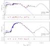 |
Fig. 1 Example of best-fit models (in black line) to the observed spectral energy distributions (SEDs) of two galaxies of our sample. One is a typical late-type galaxy (HCG2a; top panel) and the second is a quiescent elliptical galaxy (HCG62a; bottom panel). In each panel, the blue line shows the unattenuated stellar spectrum estimated by the model. The red circles are the observed broadband luminosities with their errors as vertical bars. The residuals, |

3.2. Comparison of empirical to model results
Given the available observations, the stellar mass and SFR of a galaxy are the two physical parameters that are constrained more accurately using our SED modeling. Since in Bitsakis et al. (2010) we did not had the multiwavelength data and the model, we used semi-empirical methods, relying on the K-band luminosity, to estimate the stellar mass, and the 24 μm emission for the SFR. In this section, we compare the model derived parameters with those from the empirical methods to better understand the uncertainties in the interpretation of the results. We also compare them with the methods of Salim et al. (2007) and Iglesias-Páramo et al. (2006), which use the NUV and FUV bands of GALEX, respectively, to estimate the SFR, in order to evaluate their consistency with the model results.
The stellar mass of a galaxies can be estimated using the Bell et al. (2003) prescription which was calibrated using a large sample of galaxies in the local universe. Their formula, based on the K-band luminosity, is  (1)where B and R are the B- and R-band magnitudes of the galaxy, LKs its Ks-band luminosity in units of solar luminosities (LKs, ⊙ = 4.97 × 1025 W), a = −0.264, and b = 0.138, with systematic errors of ~30% due to uncertainties in the star formation history and dust. Because these authors used “diet” Salpeter IMF, we corrected it to a Chabrier IMF (which our model uses, scaling down their M/L by −0.093 dex as described in Zibetti et al. 2009). Finally, since Bell et al. (2003) relation uses BC03 models (Bruzual & Charlot 2003), which do not take into account the contribution of thermally pulsing AGB stars, we applied the color correction as described in Zibetti et al. (2009) for the CB07 (Charlot & Bruzual 2007 libraries), where a is −1.513 and b is 0.750 for the same colors. As we can see in Fig. 2, the masses estimated by the model (Mmodel) agree with the Zibetti et al. (2009) ones. This was somewhat expected as this recipe was calibrated using the same models. However, there are some outliers, such as HCG40f, for which the model was not able to estimate the stellar mass very well since there were not enough observations to constrain its SED well.
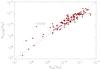 |
Fig. 2 Stellar masses based on the da Cunha et al. (2008) model (hereafter MDCE08) are plotted as a function of the ones derived from Bell et al. (2003) relation based on Ks luminosity (MKs) after applying the corrections discussed in the text. Vertical error bars indicate the 16–84 percentile ranges in the recovered probability distributions, while the horizontal error bars are the 30% errors as described by Bell et al. (2003) determined from the scatter in the models. The blue dashed line represents the one-to-one relation. |
The rate at which a galaxy forms stars is one of its most important properties, especially in interacting systems, which evolve very rapidly as they are consuming the available gas. In the absence of narrow-band imaging of the hydrogen recombination lines (i.e. Hα), two of the most common ways to estimate the SFR rely on prescriptions using their UV broad band emission from GALEX or the 24 μm thermal dust emission from Spitzer/MIPS.
Since a significant fraction of the bolometric luminosity of a galaxy is absorbed by interstellar dust and re-emitted in the thermal IR, mid-IR observations can probe the dusty interstellar medium and dust-enshrouded SFRs. The efficiency of the IR luminosity as a SFR tracer depends on the contribution of young stars to heating of the dust and the optical depth of the dust in the star-forming regions. Calzetti et al. (2007) using a wealth of multiwavelength observations for 33 SINGs galaxies provided the recipe  (2)to calculate the SFR from the 24 μm luminosities obtained with Spitzer. We used this formula to estimate the SFR of the galaxies in our sample and display them in Fig. 3. As we can see, the 24 μm estimates and those from the model fit to the whole SED agree fairly well, because they have a ratio with a median value of unity and a standard deviation of 0.51dex. The scatter does not seem to correlate with the galaxy mass or luminosity. To examine whether the scatter is due to the absence of far-IR measurements, for a large fraction of the galaxies in our sample we selected 35 galaxies for which IRAS and Akari fluxes were available and fit them again with the model, this time removing the far-IR points. We then compared the new estimates of the SFRs with the ones when all data were used and found that they were very similar, their average ratio being 0.95 and the corresponding standard deviation 0.19. A possible explanation for the scatter between the results of the model and the Calzetti et al. (2007) method could be related to variations in the metallicity of the galaxies (i.e. Rosenberg et al. 2008). Another factor that may influence the SFR values, related to the star formation history of the galaxies, is that in the da Cunha et al. (2008) model the SFRs are averaged over 100 Myr, while the Calzetti et al. (2007) assumes a timescale of 10 Myr.
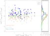 |
Fig. 3 A plot of the ratio of the SFRs derived from the observed FUV or 24 μm fluxes over the SFRs derived from the da Cunha et al. (2008) model as a function of the model SFR. Red open circles and red open triangles are the SFRs derived from the MIPS 24 μm fluxes for early and the late-type galaxies respectively. Green open circles and green open triangles mark the estimates based on the FUV to IR excess as described by Buat et al. (2005). Filled blue triangles indicate late-type galaxies for which the SFRs are derived from the FUV after estimating the extinction using the β slope method of Meurer et al. (1999). The dashed line is the one-to-one relation. The histogram of the ratios for each method is indicated in the right panel. |
In the UV the integrated spectrum is dominated by young stars, so the SFR scales linearly with luminosity; however, in order to use the UV to trace SFR, we have to correct the attenuated UV fluxes for dust extinction. One method to do this is to use the β-slope correction, 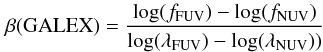 (3)where fFUV and fNUV are the flux densities per unit wavelength in the FUV and NUV bands respectively, λFUV = 1520 Å, and λFUV = 2310 Å. Then we can apply the relation of Meurer et al. (1999) to starburst galaxies,
  (4)where Lobs and Lcor are the observed and extinction corrected FUV luminosities. Finally, we can derive the SFRs using the relation of Salim et al. (2007):
  (5)for Chabrier IMF.
The SFRs of the early-type galaxies cannot be estimated using this method since the β-slope is mainly determined by the old stellar population rather than the dust extinction and thus their extinction-corrected UV luminosities are completely overestimated. Even for late-type galaxies, though, when we compare in Fig. 3 the FUV estimates of the SFR with the corresponding values obtained with the model, we find that the former are overestimated by a factor of 0.56 dex with a global scatter of 0.46 dex. We attribute this to the calibration of the extinction correction of Meurer et al. (1999), who used a sample of local UV-selected starburst galaxies with high dust content, quite dissimilar to the HCG galaxies. As discussed in detail by Kong et al. (2004), this leads to overestimating the UV corrected luminosities and consequently to an overestimate of the SFRs. Indeed, when we plot the FIR-to-UV luminosities of our galaxies against the spectral slope (β-slope), we notice that at a fixed β all the galaxies have systematically lower ratio of total to FIR-to-UV luminosities than the starburst galaxies of Meurer et al. (1999). On the other hand, galaxies HCG16c and HCG16d, which are IR luminous (LIR > 1011 L⊙), have SFRs that are very similar to those derived by the model (10.02 and 1.52 M⊙ yr-1, respectively).
Since, the previous method overestimates the SFR, we can also use the relation of Buat et al. (2005). These authors used the IR-to-UV luminosity ratio to quantify the dust attenuation in the FUV band of GALEX for a wider sample consisted of more quiescent galaxies. The formula they derived to correct for dust extinction is described by the relation  (6)where y = log (Fdust/FFUV) is the ratio of the IR-to-UV flux densities. To derive these ratios for our galaxies we used the IR luminosities estimated by our SED modeling, as well the observed UV luminosities, and estimated the SFR using the formula (4) of Iglesias-Páramo et al. (2006):
 ![Mathematical equation: \begin{equation} \log [{\it SFR}_{\rm FUV}(M_{\odot}~{\rm yr}^{-1})=0.63\times(\log [L_{\rm FUV,\,corr}(L_{\odot})]-9.51) \end{equation}](/articles/aa/full_html/2011/09/aa17355-11/aa17355-11-eq84.png) (7)where the LFUV, corr is the extinction-corrected FUV luminosity (in L⊙), and the factor of 0.63 has been introduced to correct for the Chabrier IMF (Chabrier 2003; da Cunha et al. 2008). The results are presented in Fig. 3 in green. We notice that the ratios of the SFRs are uniformly distributed around ~1.05 displaying a scatter of 0.56 dex and also agree with the 24 μm estimates. Given the success of the model in a variety of systems (see da Cunha et al. 2008, 2010a,b) we base the remaining of the analysis in the model derived SFRs.
(7)where the LFUV, corr is the extinction-corrected FUV luminosity (in L⊙), and the factor of 0.63 has been introduced to correct for the Chabrier IMF (Chabrier 2003; da Cunha et al. 2008). The results are presented in Fig. 3 in green. We notice that the ratios of the SFRs are uniformly distributed around ~1.05 displaying a scatter of 0.56 dex and also agree with the 24 μm estimates. Given the success of the model in a variety of systems (see da Cunha et al. 2008, 2010a,b) we base the remaining of the analysis in the model derived SFRs.
4. Results
4.1. Evolutionary state of the groups
To study the star formation properties of HCGs groups, Bitsakis et al. (2010) separated them into dynamically “young” and dynamically “old”. We classified a group as dynamically “young” if at least 75% of its galaxies are late-type. Conversely, a group is dynamically “old” if more than 25% of its galaxies are early-type. It is known that the sSFR is a tracer of the star formation history of a galaxy, and galaxies in compact groups do experience multiple encounters with the various group members. Consequently, we would expect that a young group is more likely to have more late-type galaxies, since its members would not have enough time to experience multiple interactions that would trigger star formation, consume the available gas, and transform them into early-type systems. Furthermore, these late-type galaxies would not get built up much of their stellar mass. They would still have larger amounts of gas and dust, as well as higher SFRs and sSFR. On the other hand, if a group is dominated by early-type systems, it would be dynamically “old”, since interactions and possible merging of its members over its history would have led to the formation of some of those ellipticals. As a result, the spirals in these groups would have already built some of their stars, and their sSFR would be lower. In our present sample, ten groups (HCG2, 7, 16, 38, 44, 47, 54, 59, 91, & 100) are classified as dynamically “young” and the remaining 22 as dynamically “old” (see Table 7).
We notice that in the majority of the groups (80%) that are classified as dynamically “old”, the most massive galaxy that dominates is an early-type galaxy displaying a median stellar mass of 1.2 × 10¹¹ M⊙. In all dynamically “young” groups, the dominant galaxy is late-type, with a median stellar mass of 5.1 × 10¹⁰ M⊙. These most massive galaxies of each group, are marked with a star in Table 4. Even though there are just ten dynamically “young” groups in our sample and we could be affected by small number statistics, we note that dynamically “old” groups have on average 4.7 members in each, more than the “young” groups, which only have four members.
A different classification of the HCGs into three phases, 1, 2, and 3, based on their HI gas content has been proposed by Verdes-Montenegro et al. (2001). In the first phase, the HI gas is mainly associated with the disks of galaxies. In the second, 40–70% of the HI is found in the disks of the galaxies, and the rest has been stripped out, due to tidal stripping, into the intragroup medium. Finally, in the third phase are groups with almost all their HI located outside of member galaxies, or in a common envelope engulfing most group members. Using this classification, Borthakur et al. (2010) classify 14 of the groups in our sample, and the results are presented in Table 7. Both ours, as well as the Verdes-Montenegro et al. (2001) classification method, are based on how galaxy interactions and merging affect the morphology of the group members, thus they are related to their evolution. There is global agreement between the two methods for 12 of the 14 groups we have in common. We discuss these in more detail in Sect. 4.6.
4.2. The physical properties of HCG galaxies
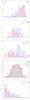 |
Fig. 4 Histograms of several properties of our HCG sample. Early type galaxies are marked in red and late type galaxies in blue: a) the distributions of the stellar masses (M ∗ ), b) the distributions of the star formation rates (SFR), c) the distributions of specific SFR (sSFR), and d) the histogram of the IR luminosities, LIR, in red, as estimated by our SED modeling. Because of the absence of far-IR observations for most of the sample, we overplot in hashed areas the histograms corresponding to the minimum and maximum LIR of each galaxy, associated to the 16th and 84th percentile ranges of the best fit, respectively, e) a histogram of the extinction inferred from the SED fit (AV, obs) as measured model-derived atttenuated and unattenuated SED (see Sect. 3.1.3). |
We now use the results of the SED modeling, described in the previous section, to examine the physical parameters of the galaxies in our sample and compare them with the ones derived for the comparison samples. The large number of galaxies, a total of 135 in 32 groups, is enough to produce statistically significant results in order to explore these parameters.
In panel a of Fig. 4 we present the distributions of the stellar masses separated in early- (E’s and S0’s) and late-type (S’s and Irr’s) galaxies in groups. We can see that the distributions are not too different because a two-sided Kolmogorov-Smirnov (KS) suggests that the probability (PKS) that the two samples are drawn from the different populations is ~0.04. The median stellar masses of the late and early-type galaxies in our sample are 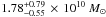 and
and  respectively. One might have expected that the late-type galaxies would have much lower stellar masses than the early-types since the latter have had more time to increase their stellar mass as they converted their gas into star and/or resulted from the merging of late type systems. However, as we know tidal interactions play an important role in triggering star formation in galaxies (Struck 1999). Compact groups have high galaxy density, display signs of interaction (e.g. Verdes-Montenegro et al. 2001), and contain galaxies that are actively forming young stars. Furthermore, as we showed in the previous section, most of the massive late-type galaxies are found in dynamically “old” groups. We thus believe that several of the HCG late-type galaxies have already increased their stellar mass, thanks to past tidal encounters. We examine these galaxies and their properties more specifically in the next section.
In Fig. 4b we present the distributions of the SFRs of early and late-type galaxies in groups. As expected, most of the late-type galaxies have higher SFRs than the early-type systems, their median SFR being 0.60 yr-1 compared to 0.05
 yr-1. The maximum SFR seen in our sample is ~26 M⊙ yr-1, typical of starbursts in the luminous IR galaxy (LIRG) range. We should note that there are eight early-type galaxies with relatively high SFRs (~1–5 M⊙/yr), which is more than an order of magnitude higher than what is observed in the rest of the sample. We discuss these galaxies in more detail in Sect. 4.4.
In panel c of Fig. 4 we display the distributions of the sSFRs of our sample. We can see that there are late-type galaxies with rather low sSFRs (~10-12 yr-1). These galaxies, which belong to dynamically “old” groups, must have had already increased their stellar masses, thus decreasing their sSFRs, as a consequence of dynamically triggered star formation events due to past interactions. On the other hand, there are early-type galaxies that display rather high sSFRs (~10-10 yr-1). One explanation is that accretion and merging of gas rich dwarf companions has increased the gas content of these galaxies, and they are currently forming stars. However, it is also possible that these galaxies are misclassified, dust obscured, edge-on late-type systems. In Sects. 4.3 and 4.4 we examine the sSFR distribution in more detail as a function of the dynamical state of each group, study the mid-IR and optical colors of the galaxies and compare them with our control samples.
In Fig. 4d we present the distribution of the LIR as estimated from the da Cunha et al. (2008) model. Since no far-IR observations were available for most of the galaxies (74%) in our sample, the LIR cannot be robustly constrained. Using the minimum and the maximum values of the probability distribution functions for each galaxy as reported by the model, we create two additional histograms corresponding to the low and high values. We observe that the overall shape and median value of the distribution does not change substantially. The median LIR of the sample is  and most of the HCG galaxies are not IR luminous (LIR ≥ 1011 L⊙). There are only seven galaxies, HCG4a, HCG16c, HCG16d, HCG38b, HCG91a, HCG92c and HCG95a, with LIR > 1011 L⊙. These are all late-type systems, and they are detected in the far-IR, and the first five are found in dynamically “young” groups.
As we discussed in Sect. 3.1.3 we can use the model-derived attenuated (observed) and unattenuated SEDs to estimate the V-band optical depth (AV, obs) for each galaxy. Two histograms of these values, for the early and late-type systems, are presented in Fig. 4d. The median AV, obs is 0.23 ± 0.17 mag and 0.58 ± 0.36 mag for the early and late-type galaxies, respectively. We observe that there are eight (~14%) of the early-type galaxies, with extinctions similar to what is seen in dusty late-type galaxies (≥ 1 mag). These are HCG4d, HCG55c, HCG56b, HCG56d, HCG56e, HCG71b, HCG79b, and HCG100a. We should note that these galaxies are the ones forming the tail of early-type galaxies with high SFRs and sSFRs, mentioned above. That they appear to have larger amounts of dust than what one may expect for early-type galaxies, as well as the fact that they display higher star formation activity, further supports the idea that these may indeed be misclassified as late-type systems.
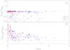 |
Fig. 5 a) Ratio of the intrinsic τV, ISM derived by the model over the observed (attenuated spectrum) τV, obs versus the τV, obs. The dashed line is the one-to-one ratio. The red circles represent the early-type galaxies in HCGs, and the blue diamonds the late-type ones. b) Ratio of the intrinsic τV for stars in birth clouds, derived by the model over the observed τV, obs versus the τV, obs, using the same notation. We excluded 6 galaxies from the plot (HCG44a, HCG47a, HCG47b, HCG56b, HCG59a, and HCG68a) since their χ2 of model-fit was more than 9.00 and the derived τ fairly uncertain (see Table 3). |
The model of da Cunha et al. (2008) also estimates the total effective V-band absorption optical depth of the dust seen by a young star (τV = τV, BC+τV, ISM) inside the stellar birth clouds, and the fraction of the absorption (μ) contributed by dust found in the diffuse ISM along the line of sight. The emission from young stars is more attenuated than from old stars. In young stars the extinction is dominated by the dust of the surrounding birth clouds with an additional component due to the dust in the diffuse ISM traversed by their light. Older stars (>100 Myr), which have dispersed their birth clouds, are only affected by the dust found in the diffuse ISM. Consequently, one would expect that in early-type galaxies, where currently no recent star formation is taking place, the optical light would be dominated by the old stars, and therefore, the representative obscuration would be that of the ambient ISM. In late-type galaxies the total extinction would be the contribution of both components, BC and ISM. In that case, each component will contribute differently, depending on how much of the optical energy production in the galaxy is due to stars within the birth clouds. We would like to emphasize that since both components can contribute to a different extent at different wavelengths, the representative extinction of a galaxy also varies with wavelength, and that is why we consider only optical light here, instead of referring to the total energy output of the galaxy.
Using the output of the model, we can thus estimate the optical depth contributed from the diffuse ISM, τV, ISM = μ τV, and the optical depth from the stellar birth clouds, τV, BC = (1 − μ) τV. In Table 4 we present the optical depth derived from the attenuated and unattenuated SED, τV, obs, the τV, ISM, as well as the total optical depth seen by young stars inside stellar birth clouds, τV = τV, BC + τV, ISM. In Fig. 5, we plot the ratios of the intrinsic, model-derived optical depth (ISM and BC+ISM components) versus the observed optical depth, τV, obs, that we measured from the SED. We note that in most galaxies the ratio of τV, ISM over τV, obs is very close to unity. For these galaxies, in particular for those with low extinction values, it is the dust in the ISM that determines the overall absorption of the emitted radiation. The contribution of the BC component is a small fraction of the overall light. On the other hand, there are 28 galaxies with ratios lower than unity. From these, 18 are classified as late-type, half of them belong to dynamically “young” groups, and ten are classified as early-type, six of which we believe are likely misclassified late-type systems (see Sect. 4.4 and Appendix). In the bottom panel of the same figure we plot the ratio of total τV over the τV, obs, versus the τV, obs. We notice that there are galaxies with very high τV over τV, obs values at small τV, obs, most of which are early-type systems. Even though these galaxies have had recent (<100 Myr) star formation events, this does not dominate their global emission. We do note, though, that as the τV, obs increase, the ratio converges towards unity, implying that the contribution of light from young stars in the BC component becomes a considerable fraction of the total emission, making the obscuration seen by the newly formed stars more representative of the observed obscuration of the galaxy.
4.3. HCG late-type galaxies
It is well established that interactions can trigger star formation in galaxies (i.e. Struck 1999). During an interaction between two late-type galaxies, their atomic gas, as is typically found in diffuse clouds, collide. Shocks are produced that in turn increase the local gas density, thus triggering bursts of star formation. That the group environment has played an important role in the evolution of its member galaxies is evident since the fraction of early-type systems in groups is higher that what is found in the field, so one would expect that, because of their proximity, the late-type galaxies in groups would display different star formation properties from the ones in the field. However, in a preliminary analysis of 14 groups, Bitsakis et al. (2010) found that overall there is no evidence that the SFR and sSFR in late-type galaxies of HCG is different from galaxies in the field or in early-stage interacting systems. Interestingly though, when they separated their HCG sample into two subsamples, namely the dynamically “old” and dynamically “young” groups (see Sect. 4.1 for the definition), late-type galaxies in dynamically “old” HCGs showed lower sSFRs than those in dynamically “young” groups. This was attributed all the likely past interactions experienced in the dynamically “old” groups, which would lead to a faster increase in their stellar mass compared to galaxies in young group. The higher stellar mass would reduce their current sSFR, even if subsequent gas accretion would result in star formation activity in them.
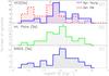 |
Fig. 6 Histograms of the sSFR of the late-type galaxies our three samples, estimated by modeling their SED. The top plot displays in blue the histogram of the sSFR of the 31 late-type galaxies found in dynamically-young, spiral-dominated groups. Overplotted in red is the corresponding histogram of the 42 galaxies in dynamically-old elliptically dominated groups. The middle and bottom plots present the histograms of the 52 late-type galaxies in the Smith et al. (2007a) interacting galaxy pairs, as well as the 71 SINGS late-type galaxies. The arrows indicate the median sSFR value of each distribution. |
We re-examined this issue using our larger sample of 32 groups that contains 73 late-type galaxies and derived their sSFR, as well as the one of the control samples, using the SED model of da Cunha et al. (2008). The results are shown in Fig. 6 and Table 3. Galaxies in dynamically “young” groups have a median sSFR of 8.51 yr-1, while s
 yr-1 for galaxies in the dynamically “old” groups. Similarly, galaxies in interacting pairs have an s
 yr-1 and in field galaxies s
 yr-1. An analysis using a two-sided KS test indicates that there is no statistical difference between the samples of late-type galaxies in dynamically “young” HCGs and those of the SINGs and interacting pair samples (PKS > 0.80). However, the same KS test reveals that the late-type galaxies in dynamically “old” groups, with a median sSFR that is more than three times lower, cannot be drawn from the same parent distribution as the three other samples (PKS ~ 10-3). Investigating in more detail the reason for this disparity, we find that it cannot be attributed to depressed SFR, but instead it is due to a substantially more massive stellar content (~3 × 10¹⁰ M⊙), similar to what is found in early-type systems. This confirms the results and interpretation of Bitsakis et al. (2010), who relies on semi-empirical estimates of the sSFR on a smaller galaxy sample. Based on those findings one would also expect that owing to their higher stellar mass, the late-type type galaxies in dynamically “old” groups should have redder UV and optical colors than late-type galaxies in the field. We examine this in Sect. 4.5.
4.4. HCG early-type galaxies
We showed in the previous section that the group environment affects the star formation history of the late-type members by increasing their stellar mass in the process of transforming them into early-type systems. However, is there any evidence that the early-type galaxies in groups are distinctly different from similar galaxies found in the field? Based on our SED modeling, we have already shown in Fig. 4 that nearly 15% of all early-type galaxies have SFRs and dust extinction similar to what is seen in late-type systems. We suggested that there are two possible explanations for this. One was that they were simply misclassified as Es or S0s, while they are edge-on in fact late-type systems. The second was that even if they are early-type, based on their optical morphology, these galaxies they have experienced minor merging with gas/dust rich dwarf companions in the groups, which has increased their gas content, star formation activity, and dust extinction.
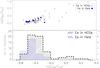 |
Fig. 7 Top panel: IRAC color–color plot of the early-type galaxies in HCGs (black open triangles) and a sample of field ellipticals (blue filled circles). Bottom panel: the histograms of the log[S5.8/S3.6] color of the two samples. The early-type galaxies in the groups are marked with a black line (left axis), while the field ellipticals are presented in blue (right axis). |
According to Hickson (1982) the classification of the HCG galaxies was performed using their morphological features, optical colors, and sharpness of the edge of the image. For all groups of our sample, though, we also have Spitzer mid-IR images that provide additional information on their properties. It is well known that the mid-IR spectra of the star-forming galaxies, in addition to continuum emission due to warm dust, are also filled with a series of broad emission features between 3 and 18 μm, which can contribute up to 20% of their total IR luminosity (Dale et al. 2005; Smith et al. 2007b). These features are the vibrational modes of polycyclic aromatic hydrocarbons (PAHs), which absorb UV photons from newly born stars and re-emit them in the mid-IR. Typically only late-type galaxies with active star formation and dust emit strongly in these bands. Some PAHs have also been detected in some early-type systems, but they display peculiar PAH-band ratios (Bressan et al. 2006; Kaneda et al. 2008; Panuzzo et al. 2011).
To probe the properties of the early-type galaxies in the groups, we examined their mid-IR colors and compare them with isolated ellipticals in the field, which are not expected to have PAH emission. In Fig. 7 we use our Spitzer/IRAC photometry and plot the 8.0 to 4.5 μm flux density ratio as a function of the 5.8 to 3.5 μm ratio for both the early-type galaxies of our HCG sample, and the control sample of field ellipticals. Weak PAHs would result in low values of both ratios since the 6.2 and 7.7 μm features, which contribute ~50% of the total PAH emission, are sampled by the 5.8 and 8.0 μm IRAC filters (Smith et al. 2007b). Indeed, we observe that most of the early-type galaxies in groups, as well as in the field, are concentrated in the lower left hand part of the color–color plot of Fig. 7. These galaxies are very close to the (− 0.4,−0.5) locus of pure stellar photospheric emission where the flux density in the mid-IR scales with λ-2. Consequently, they are expected to have very weak dust and PAH emission. On the other hand, the upper right quadrant of the figure should be populated by galaxies with strong PAH features and possibly some hot dust contribution, as a result of intense star formation and/or AGN activity. As expected, no field ellipticals are seen in this quadrant. However, there is a “tail” of ten early-type HCG galaxies (~16% of the total) extending to this part of the plot (for log [f5.8/f3.6] > −0.25). Examining the 5.8 to 3.5 μm IRAC color distributions of HCG and field with a KS test, we find that they are different (PKS ~ 0.005). The early-type galaxies with red IRAC colors are HCG4d, HCG40f, HCG55c, HCG56b, HCG56d, HCG56e, HCG68a, HCG71b, HCG79b, and HCG100a. We note that HCG40f and HCG68a are at the left hand edge of the color selection, and it is possible that contamination from a red nearby companion is affecting their mir-IR fluxes. All these galaxies are examined in more detail in the Appendix, where we display their SEDs, Ks-band contour plots, and “true color” composites based on their Spitzer/IRAC mid-IR images. Based on this analysis and previous suggestions, we propose that seven of them, HCG4d, HCG55c, HCG56d, HCG56e, HCG71b, HCG79b, and HCG100a are likely dust-obscured late-type systems. Furthermore, if HCGd and HCG71b are indeed late-type galaxies, then their groups must be reclassified as dynamically “young” (instead of “old”). In the rest of this paper we consider them as such (see Tables 6 and A.1).
4.5. Bimodality in HCG galaxy colors
In the previous sections, we have examined several of the physical parameters of our HCG sample as derived by the SED modeling. To examine the evidence of evolution due to the group environment more thoroughly, we now compare all our results based on the UV, optical, and IR imaging, as well as the available spectroscopic diagnostics.
Several studies of galaxies have revealed a bimodality in the UV-optical colors of galaxies in field and in clusters (e.g. Wyder et al. 2007; Haines et al. 2008). This type of bimodality in the colors of the late- and early-type galaxies is real and directly connected to the original galaxy classification scheme by Hubble. It appears quite strongly in the NUV-r color distribution of a sample and consists of two peaks, called the “red sequence” and the “blue cloud”, and a minimum in between them identified as the “green valley” (see Strateva et al. 2001). Wyder et al. (2007) have examined a sample of over 18 000 galaxies observed with GALEX and SDSS and showed that an NUV-r versus Mr color magnitude diagram can be used to separate them into (i) passively evolving, (ii) star-forming and (iii) AGN components. Passively evolving galaxies are confined to the “red sequence” (NUV-r > 5), with few showing blue UV-optical colors, while all blue galaxies, with NUV-r < 3, are spectroscopically classified as star forming (see also Haines et al. 2008). AGN seem to dominate the area of the green valley” (3 < NUV-r < 5). The small fraction of galaxies in the “green valley” can be understood from the fact that galaxies do not spend so much time at these colors. Using Starburst99 (see Leitherer et al. 1999) we simulated the evolution of a stellar population typical of a spiral galaxy assuming solar metallicity and either a continuous star formation (of 1 M⊙ yr-1) or a single starburst (producing total stellar mass of 106 M⊙). Depending on the assumptions, we find that the colors of the population place it within the “blue cloud” just for ~5–7 Myr, and after spending only ~1–5 Myr transiting through the “green valley”, it remains in the “red sequence” for the rest of its lifetime. Thus this color bimodality emerges from the nature of the galaxies as they evolve through time.
In Fig. 8 we plot the NUV-r colors of our HCG sample, and compare them with the field and cluster galaxies of the Haines et al. (2008) sample. The three regions of the color space discussed by Wyder et al. (2007) are clearly visible. On the left, near NUV-r ~ 2, we identify the “blue cloud” where the field galaxy distribution peaks. Nearly 58% of the total number of field galaxies is found within 0.5 mags of this color. Few of the galaxies in clusters (15%) are also seen in this area. To the right, near NUV-r ~ 5.5, we observe the “red sequence” where most (51%) of the cluster galaxies are concentrated. Only 16% of the field galaxies are found in the “red sequence”. The “green valley” is between the two peaks and is mostly (34%) populated by cluster galaxies (Haines et al. 2008). When we examine the HCG NUV-r color distribution, we note a clear difference. Only 17% of their galaxies are in the “blue cloud”, a fraction similar to what is found for galaxies in clusters. However, the majority (73%) of the HCG galaxies are concentrated in the “green valley” and “red sequence” areas. A likely explanation would be that most of the HCG galaxies are already passively evolving or that they are in the process of moving from the star-forming region to the “red sequence”. This is consistent with compact groups having a higher fraction of elliptical galaxies than the field. Another possibility is that some of these galaxies are in fact late-type systems that have redder colors so move to the right on the plot, because of dust extinction or the presence of a substantial older stellar population (post starburst galaxies), or both. This is expected from our earlier findings regarding the missclassification of a fraction of the early-type galaxies in the HCG and the lower sSRF in dynamically “old” groups.
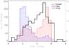 |
Fig. 8 NUV-r histogram of our HCG galaxy sample shown in black (right Y-axis). The histograms of the field, in blue, and cluster galaxies, in red, from the Haines et al. (2008) control sample are also presented (left Y-axis). |
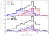 |
Fig. 9 a) NUV-r histogram of the whole HCG galaxy sample is shown in black. The corresponding histograms of the early- and late-type galaxies of the sample, classified according to their optical morphology, are shown with the red and blue shaded areas. b) The NUV-r distribution of the galaxies hosting an AGN is indicated with the dashed dark line. As above, the early- and late-type hosts are indicated with the red and blue histograms. The region of 3 < NUV-r < 5, identified as “green valley”, is marked with the vertical dashed lines. |
To study in more detail how the NUV-r color distribution of the HCG galaxies is affected by their morphology and nuclear activity, we present in Fig. 9 the corresponding histograms based on their optical morphologies, as well as their nuclear spectral classification. We note that only 36% of the late-type galaxies are found within the “blue cloud”; however, the majority of the HCG galaxies, almost 60%, are located in the “green valley” and in the “red sequence” (~13%). In Fig. 9b we present the same plot as at the top, but only for the galaxies of our sample that have an optically identified AGN. The whole distribution is shown, while the distributions of early- and late-type AGN hosts. We performed a two-sided KS test between the distribution of galaxies hosting an AGN and the total distribution of the HCG galaxies, and we conclude that there is no statistical difference in their NUV-r colors (PKS ~ 0.25). This suggests that the presence of an AGN does not substantially affect the UV-optical color of the galaxies in HCGs.
As we described earlier, more than 40% of the galaxies in our sample host an AGN in their nucleus. This, in addition to the code of da Cunha et al. (2008) not including the contribution of an AGN to the SED of a galaxy, could bias some of our results, in particular the SFR, sSFR, and the LIR. Using the IRAC color–color AGN diagnostics introduced by Stern et al. (2005), we investigated the influence of the AGN to the mid-IR SED of the galaxies in our sample. Only three systems, HCG6b, HCG56b, and HCG92c, have mid-IR SEDs that are consistent with a strong power-law continuum emission, which indicates a strong AGN in their nucleus. For all remaining galaxies, the optically identified AGN does not dominate their SED, so that their physical parameters estimated by our model are considered reliable.
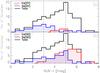 |
Fig. 10 a) NUV-r histogram of our HCG galaxy sample shown as a black solid line. The corresponding histograms of the early- and late-type galaxies found in dynamically “young” groups are shown with the red and blue shaded areas, respectively. b) Same as in a), but for the galaxies in dynamically “old” groups. The region of 3 < NUV-r < 5, identified as “green valley”, is marked with the vertical dashed lines. |
To explore the color variations as a function of the evolution state of the groups, we plot in Fig. 10 the histograms of the early- and late-type galaxies found in the dynamically “young” and “old” groups, respectively. Observing the top panel we find that almost 60% of the late-type galaxies in dynamically “young” groups are located within the “blue cloud”, and 43% of them, for which nuclear spectra were available, host an AGN in their nucleus. There are also three outlier galaxies (HCG16b, HCG44a, and HCG59a) that have red NUV-r colors (>5 mag). It is possible that these systems have built up their stellar mass in the past and that their UV/optical colors are currently dominated by emission from old stars. In addition, past tidal interactions probably stripped some of their gas in the intragroup medium, thereby decreasing the fuel necessary for current star formation. In dynamically “old” groups, the late-type galaxies are redder, and as we can see in Fig. 10b, most of them (>63%) are located within the “green valley”. As in dynamically “young” groups there are also four galaxies (HCG22b, HCG40d, HCG68c, and HCG71a) in these groups, which are found in the “red sequence”.
Overall 45% of the early-type galaxies, shown in red in Fig. 9, are located within the “red sequence” and the rest are along the “green valley”. As we mentioned earlier, these systems are expected to be passively evolving and thus, their colors should be dominated by old stellar populations. We find that this is the case for most of them, as only two are found in the “blue cloud”. We believe that these galaxies are misclassified, as late-type galaxies (see Sect. 4.4), and we examine them in more detail in the Appendix. From Fig. 10a we see that all early-type galaxies in the dynamically “young” groups are in the in the “green valley”. One could suggest that they were already early-type before reaching the group, and the interactions and/or merging of dwarf companions in the group environment triggered the star formation activity and provide extra gas. However, the most likely explanation is that these are group galaxies that are currently migrating from the “blue cloud” to the “red sequence”. In that case, the morphological transformation should accompany the color transformation. Indeed, the galaxies located in bluer colors (around NUV-r ~ 4) are lenticulars, while the ones at NUV-r ~ 5 are ellipticals. Similarly, in the bottom panel of Fig. 10 we see that more than half of the early-type galaxies in dynamically “old” groups are located within the “green valley”. These galaxies are mostly (>70%) S0/SB0’s. However, there is a large fraction (~25%) of elliptical galaxies that have the same colors. We suggest that, even though the morphology of a galaxy typically determines its colors, there are several of the group ellipticals that move back to bluer colors due to interactions and/or merging in the compact group environment.
 |
Fig. 11 A histogram of the NUV-r colors of the HCG sample after correcting for dust extinction, in shown with the black solid line. The separation in two panels for “young” and “old” groups as well as the symbols follow the notation of Fig. 10. |
As discussed before, we know that the UV-optical colors of a galaxy, are not only affected by its star formation history, but also by dust extinction. Thus, it would be useful to understand how much of the observed variation in colors is due to intrinsic extinction in the galaxies. Especially for the late-type galaxies, which are located within the “green valley”, we have to examine whether their colors are affected more from dust or whether it is because they contain a substantial old stellar population. Our SED model allows us to estimate and to correct for dust attenuation, so we plot in Fig. 11 the distributions of the corrected NUV-r colors of the early- and late-type galaxies in dynamically “young” (top panel) and dynamically “old” groups (bottom panel). We notice in panel a) that almost all late-type galaxies in “young” groups move back to the “blue cloud”, suggesting that it is the dust that plays a dominant role in their apparent colors. On the other hand, 40% of the late-type galaxies in dynamically “old” groups still remain in the “green valley” after the extinction correction. It seems that in those it is the old red stars that dominate their UV/optical colors. This also agrees with the results of Sect. 4.3 where these galaxies display low sSFRs. Moreover, one can notice the large fraction of early-type galaxies that, after the extinction correction, move to the “green valley” (~50% of the galaxies at these colors). These galaxies display high sSFRS (~0.21 × 10⁻¹¹ yr-1), so their bluer colors are possibly due to higher levels of current star formation. We should note that even though for most galaxies the observed optical extinction derived from the SED model (AV) is not very high (see Fig. 4e and Table 3), this translates to over 2 mags of correction in the NUV due to the steepness of the extinction curve.
Since dust appears to affect the UV colors of HCG galaxies, one could suggest the use of their mid-IR colors, because they trace the light that was originally absorbed by the dust grains in the UV-optical. In Fig. 12 we present the IRAC color–color diagram, also shown in Bitsakis et al. (2010), using our new, larger sample. The physical meaning of this plot was described extensively in Fig. 7. We notice that most of the late-type galaxies are located in the upper right quadrant of the plot, while most of the early-types are in the lower left. The ten early-type galaxies that display red mid-IR colors are the ones we mentioned in Sect. 4.3. We observe that between the colors −0.1 < log [f8.0/f4.5] < 0.3 and −0.25 < log [f5.8/f3.6] < −0.10, there is a lower density of galaxies. Johnson et al. (2007) and Tzanavaris et al. (2010) propose that this “gap” is related to an accelerated migration of the galaxies from star forming to quiescent. When we compare this result to Fig. 11 we notice that the galaxies in the upper right quadrant of the IRAC color–color plot are the ones with NUV-r < 2.5, while galaxies located in the lower left portion of the figure have NUV-r > 3.5. We finally notice that the lower galaxy density area appears in both figures and actually separates the star forming (“blue cloud”) from the passive evolving (“green valley” and “red sequence”) galaxies. Therefore we suggest that the color bimodality observed in the extinction-corrected UV-optical colors is also observed in the mid-IR and possibly emerges from the same physical properties of the galaxies.
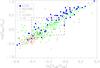 |
Fig. 12 The IRAC color–colors plot, originally presented in Fig. 7. Blue circles indicate the spiral galaxies of our HCG sample, blue squares are the irregulars, red triangles are the elliptical galaxies, and red diamonds the lenticular ones. Green dots indicate the LVL galaxies. According to Johnson et al. (2007) the “gap” is located in the area enclosed by the dashed lines. |
How significant is this “gap”? Walker et al. (2010) compared their sample of 12 HCGs with several control samples including the SINGS and interacting pair sample we used, as well as galaxies from the Coma cluster, and the local legacy volume sample (LVL Dale et al. 2009). They conclude that the mid-IR color distribution of HCG galaxies is not seen in the field, but it is seen in galaxies of the Coma infall region. However, in their analysis they combine the SINGS and LVL galaxies as a single local galaxy sample. As we mentioned, though, in Sect. 2.6.1, the SINGS sample was selected to explore the mid-IR properties of various galaxy types seen in the local universe, but it is not representative of a flux or volume limited population (Kennicutt et al. 2003). This selection biases the statistics of the colors of the sample. In contrast, the LVL sample is volume limited, since it contains all known galaxies inside a subvolume of 3.5 Mpc and an unbiased sample of spiral and irregular galaxies within the larger, more representative, 11 Mpc volume. The mid-IR colors of the LVL sample are plotted in Fig. 12. Performing a two-sided KS-test between the distributions of the IRAC colors (log[f8.0/f4.5] and log[f5.8/f3.6]) of HCG and LVL samples, we find that the distributions are not significantly different displaying PKS = 0.035 and PKS = 0.028, respectively. This suggests that there is no strong evidence that an accelerated evolution of galaxies in HCG is responsible for a significant fast change in their global mid-IR colors.
4.6. Dynamical properties of HCG galaxies
As we mentioned in Sect. 4.1 we classified the dynamical state of our sample depending on the fraction of elliptical galaxies they contain. Our method is related to their evolution since it is known that galaxy interactions and merging, transform galaxies from late-type systems to ellipticals. Thus, groups with excess of early-type members are likely to be older and more compact. To investigate this, we estimated the projected distance of each galaxy from the other members of the same group members, as well as the virial radius of each galaxy. To calculate the projected distance between the group members we used the great circle distance relation. Then, using the relation described in Park & Hwang (2009), we estimated the virial radius with the formula  (8)where L = 10−0.4(Mr + 20.00) is the r-band luminosity in L⊙, Mr the absolute r-band magnitude of the galaxy, γ the mass to light ratio (1 or 2 for late- and early-type galaxies, respectively), and ρm = 0.0223 h3 Mpc-3 is the mean density of the universe, with h = 0.72 and Ωm = 0.27. Keeping in mind that compact groups may not be fully virialized dynamical systems, we present our results in Table 6. We note that, indeed, the member galaxies are statistically closer to their nearest neighbors in dynamically “old” groups, having a mean projected distance of 26 kpc compared to 37 kpc for the dynamically “young” groups.
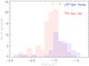 |
Fig. 13 Histograms of the “strength” of the dynamical interaction felt by each group galaxy (⟨ R/rvir, nei ⟩ /n). As usual, we separate our sample into dynamically “young” (blue) and dynamically “old” (red) groups. The arrows indicate the median values of the two distributions. |
However, galaxies in groups are interacting not only with their nearest neighbors, but also with all other group members, since in all cases the virial radii of the galaxies are substantially larger than the linear size of their group (see Table 6). To better quantify this effect we followed the approach of Hwang et al. (2010) by introducing the parameter of the “strength” of the interaction (⟨ R/rvir, nei ⟩ /n). This is estimated by averaging the ratios of the projected distances over the virial radii for all the neighbors of each galaxy and divide them by the total number of neighbors (n). This quantity provides an empirical measure of the interaction strength each galaxy experiences from its companions. The smaller this parameter, the stronger the dynamical influence of the companions.
In Fig. 13, we plot the distributions of the strengths according to the dynamical state of each group. Since we have SDSS data for only 74 galaxies and Eq. (6) relies on the SDSS r-band magnitude to compute the virial radius, we used the SED model fits to estimate the synthetic r-band magnitudes for the remaining of the sample. We observe that the “strength” parameter of dynamically “old” groups is indeed smaller than in dynamically “young” groups, suggesting that in the former the gravitational effects are stronger. A KS test between the two distributions confirms that the two distributions are significantly different (PKS ~ 10-5). Moreover, if we compare our results with the findings of Hwang et al. (2010), we see that the distances between the galaxies in groups and those of the centers of rich clusters are similar (both have R < 0.5 rvir). We can also estimate the velocity dispersion, σr, of each galaxy from the most massive-central galaxy of its group, using the published velocities from Hickson et al. (1992). Galaxies in dynamically “old” groups display mean velocity dispersion of 408 ± 50 km s-1, which is the half of what is observed in the Virgo cluster, in contrast to those in dynamically “young” groups which is about 132 ± 39 km s-1. All these facts lead us to the conclusion that dynamically “old” groups, as their name implies, are older, denser, and more evolved systems, since their properties are intermediate between those of rich clusters and dynamically “young” groups.
To further examine the dynamical properties of these groups, we can calculate their dynamical masses using the projected mass estimator from Bahcall & Tremaine (1981):  (9)where ui is the difference in the recessional velocity between the group member i and the central massive object (see Table 4 where the most massive objects in each group are marked with a star), Ri is the projected distance from the central object, and N is the number of group members. This dynamical mass can be compared to the various components of the baryonic mass of the groups. The stellar mass is derived from our SED modeling, while the total atomic hydrogen mass, MHI, is available for 29 of the groups from Verdes-Montenegro et al. (2001). Unfortunately, the mass of the molecular hydrogen, MH2, is only available for 12 groups (Martinez-Badenes et al. 2011). We note that, even though the integrated masses of the molecular and atomic hydrogen of the groups are often similar, on average they are both ~25 times less massive that the stellar component. These results are summarized in Table 7. In Fig. 14 we separate our 32 groups in the two subsamples of dynamically “young” and “old” groups and present the corresponding histograms of the distributions of their atomic hydrogen, stellar, and dynamical masses.
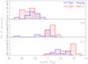 |
Fig. 14 a) Distributions of the total HI masses in the dynamically “young” (in blue) and the dynamically “old” (in red) groups, of the total stellar masses (panel b)) and the total dynamical masses (panel c)). |
We observe that the stellar mass distribution of dynamically “old” groups, shown in Fig. 14b is markedly different from for dynamically “young” groups. A KS test confirms this, as the probability that the two are drawn from the same parent distribution is PKS ~ 0.009. The median stellar mass of the dynamically “old” groups is ~1.95 × 10¹¹ M⊙, more than double what is seen in the “young” group subsample (~8.90 × 10¹⁰ M⊙). This is understood on the basis of our classification scheme; dynamically “old” groups do have more elliptical galaxies, which are typically more massive than spirals. Furthermore, from the analysis of Sect. 4.3, we have shown that the late-type galaxies of these groups also have redder optical colors.
Surprisingly, though, in Fig. 14a we note that the HI mass distribution is fairly similar in both subsamples (PKS ~ 0.26), with a median value of HI mass ~3.2 × 10⁹ M⊙. Assuming that dynamically “old” groups are older structures, with more early-type members that have already converted during a merging process a fraction of their gas into stars, it is not clear that what we see is a real “conspiracy”, given the difference in star formation properties and relative amount of old stellar populations of the two subsamples. We know that a fraction of the HI gas is expelled from the galaxies to the intragroup medium in the form of plumes, and long filaments as a group evolve progressively, transforming the morphology of its members from late- to early-type (Verdes-Montenegro et al. 2001). However, the lifetime of these structures before they either change phase, as they interact with the hot intragroup gas, or are accreted back to the group members is not well constrained, since only a dozen of HCGs have high spatial resolution maps of their gas component.
Examining the distributions of the dynamical masses of the two subsamples in panel c of the same figure, we find that, as was the case with the stellar mass, these are also different (PKS ~ 0.008). The dynamically “old” groups display a median dynamical mass of 6.46 × 10¹² M⊙, nearly an order of magnitude higher from what is seen in the “young” ones (4.77 × 10¹¹ M⊙). The dynamical masses do not simply scale with the stellar mass of the subsamples, which only differ by a factor of ~2. Furthermore, there is no indication of a variation in the ratio between the dark matter, as probed by the kinematics, and the baryonic matter in groups, or that there is a systematic error in the estimates of the dynamical mass due to one subsample being less virialized than the other. As a result, one could attribute the deficit in the observed baryons in the dynamically “old” to a component of hot intragroup gas, since there is clear evidence that groups with more early type systems have stronger X-ray emission (Ponman et al. 1996; Mulchaey et al. 2003).
In Table 7 we also present our classification of the 32 groups, based on the fraction of the early-type members, as well as the classification based on their HI morphology proposed by Verdes-Montenegro et al. (2001) for 13 groups where this was available. Despite the small number statistics, we note that there is overall agreement. Groups that we consider as dynamically old are in Phase 3 or 2 according to their HI content, while groups that we consider dynamically “young” are in Phase 1 or 2. There are two exceptions in this. HCG79, the so-called “Seyferts’ Sextet” was classified by us as dynamically “old”, but it is Phase 1 based on the distribution of its HI gas by Borthakur et al. (2010). Inspecting it closely we see that our definition is probably marginal as the system does not have an elliptical galaxy and its two early-type members are peculiar S0s. The other case is HCG44, which was classified as Phase 3 by Borthakur et al. (2010). The group consists of three late-type galaxies and NGC 3193, an E2 which Aguerri et al. (2006) argue that may be an interloper. Close inspection of the HI map of the group shown in Fig. 2 of (Williams et al. 1991) reveals that nearly all gas emission is associated with the three late-type systems, and only a small fraction is seen outside the galaxy disks. We would thus argue that this system is more likely in Phase 1 or 2, which would be consistent with our classification as dynamically “young”. Therefore, as expected, a change in the galaxy morphology also carries a change in the distribution of the atomic hydrogen within the group, and vice versa.
4.7. Diffuse cold dust in the intragroup medium
We mentioned earlier that by using the model of da Cunha et al. (2008) we were able to derive several of the physical properties of the galaxies in our sample. Even though a number of parameters, such as stellar mass and SFR, can be estimated with good accuracy, the lack of deep high spatial resolution wide field far-IR imaging, makes it very challenging to constrain the LIR and accurately estimate the amount of cold dust in each galaxy.
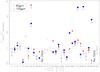 |
Fig. 15 Plot of the ratio of the observed IRAS 60 and 100 μm fluxes of each group divided by the corresponding flux all group members as predicted by our model fits. Since IRAS did not resolve/detect all the members of each group, several of the ratios are indicated as upper limits. Filled symbols indicate dynamically “old” groups. |
As described in Bitsakis et al. (2010), there are several reasons to expect that the interactions among group members have expelled diffuse cold dust along with atomic gas in the intragroup medium. In this preliminary work we had investigated the contribution of each galaxy to the total far-IR emission of its group and identified nine of the 14 groups, in which extended cold dust emission may be present. In the present work, using our larger sample of 32 groups and the physical model of da Cunha et al. (2008), we have repeated the same analysis. In Fig. 15 we plot the fraction of the integrated IRAS flux densities at 60 and 100 μm for each group as measured by Allam et al. (1996) divided by the sum of the flux densities of all group members predicted by our SED model fit. The results are presented in Table 7. We identify 13 groups (HCG6, 7, 16, 25, 55, 57, 67, 68, 71, 75, 79, 91, and 95) where diffuse cold dust emission may be present. These results agree with the previous of Bitsakis et al. (2010) with HCG37 be the only exception. Moreover, ten of these groups are dynamically “old”. This agrees with the notion that dynamically “old” groups are more evolved and their members have experienced more encounters enriching the intragroup medium. It is possible that part of the apparent far-IR excess is due to the uncertainties introduced by our SED fits. Only far-IR imaging with the Herschel Space Telescope will enable us to reliably characterize the composition and structure of the intragroup medium, as well as study the evolution of the cold dust in these systems.
5. Conclusions
In this paper we have presented the first multiwavelength analysis, from the UV to the IR, of the 135 galaxies that are members of 32 HCGs and studied the influence of the group environment in their evolution. Based on the theoretical modeling of their SEDs we conclude the following
-
The classification of the evolutionary state of HCGs according to the fraction of their early-type members appears to be physical and is in general agreement with previous classifications. The study of their properties suggest that dynamically “old” groups are more compact and have higher velocity dispersions. They also display higher stellar masses than the “young” ones, while both have similar HI mass distributions. However, “old” groups have nearly an order of magnitude higher dynamical masses than “young” groups.
-
The late-type galaxies in dynamically “old” groups display lower sSFRs since the multiple past interactions have already converted a fraction of their gas into stars, thereby increasing their stellar masses. This is also the main reason for these galaxies showing redder NUV/optical colors than field spirals. However, there are few spiral galaxies in these groups that display even redder colors. They all have very low SFRs, similar to early-type systems. We speculated that tidal interactions must have stripped the gas out of their disk suppressing their star formation activity.
-
Most early-type galaxies in dynamically “old” groups, seem to migrate from the star-forming to the quiescent galaxy colors, even though a fraction of them (~25%) display bluer colors and higher star formation activity than normal field ellipticals, possibly owing to gas accretion from other group members, as well as, to the merging of dwarf companions.
-
Late-type galaxies in dynamically “young” groups have similar star formation properties to field, and early-stage interacting pair spiral galaxies.
-
Even though nearly 46% of the HCG members have an optically identified AGN, we find no evidence either of enhanced AGN activity at any stage of the group’s evolution or of the optical/mid-IR colors of the galaxies.
-
Our analysis suggests that the reported lower density of galaxies in the IRAC color–color diagram is caused by the morphological natural bimodality of galaxies, and it is similar to what is also observed in the UV-optical colors.
-
Our SED model suggests that in 13 groups, ten of which are dynamically “old”, there is diffuse cold dust in the intragroup medium.
-
There are ten galaxies with mid-IR colors, SEDs, and star formation properties that are inconsistent with their optical classification as early-type systems. We suggest that seven of them are likely to be nearly edge-on late-type galaxies that were misclassified owing to their small size and dust extinction.
Online material
The morphological type and derived physical parameters based on the SED modeling of the HCG galaxies.
continued.
Derived physical parameters based on the SED modeling of the interacting pair’s galaxy sample.
Distance to, virial radius, and morphology of the nearest neighbor, as well as “strength” of interaction for the HCG galaxies.
continued.
Observed and predicted 60 μm and 100 μm IRAS fluxes for each group, as well as total HI, H2, stellar, and dynamical masses.
Appendix A: Peculiar early type systems
As mentioned in Sect. 4.4, there are ten peculiar early-type galaxies that display “red” mid-IR colors. It was suggested that they could either be misclassified late-type systems or that they are indeed early types that have increased their gas and dust owing to interactions and merging with companion galaxies. As discussed in Sect. 4.2, some of them display high Av, SFR, and sSFR. In this section we present all available evidence and discuss their properties in detail.
To better probe their morphology, we first examine how the old stellar populations, traced by their near-IR emission, as well as the warm dust seen in the mid-IR are distributed in each galaxy. In Fig. A.1 we present the “true color” images constructed using the Spitzer/IRAC 3.6, 4.5, and 8.0 μm maps as the blue, green, and red channels, respectively. We also include contour maps of the Ks emission for these galaxies. Bona fide early-type systems should be relaxed dynamically with an R1/4 radial profile and elliptical structure in their stellar light emission. Furthermore, they should not display star formation or color gradients, so no variation would be expected in their mid-IR “true color” images. Indeed, when one observes the “true color” image of NGC1404 (a typical field elliptical galaxy), no obvious mid-IR color gradient is seen, while the contours of the Ks-band emission, dominated by the old stellar population, are concentric ellipses. HCG40f and HCG68a also display similar mid-IR colors and profiles with the second having Ks contours consistent with a lenticular galaxy; however, the rest of the early-type HGC galaxies show either color gradients or patchy emission in their “true color” mid-IR images, which indicate possible on-going star formation warming up the dust and exciting the PAH molecules in these wavelengths. In particular the galaxies HCG4d, HCG55c, HCG56d, HCG71b, and HCG79b display reddish colors that imply stronger 8 μm emission. In HCG100a the 8.0 μm emission seems to emerge from two spiral-like structures, yet it appears relaxed when we closely examine the distribution of their old stellar population. With the exception of HCG56b and HCG71b, which display a barred-like structure, no other system shows obvious signs of spiral or irregular structure, even though it would have been challenging to identify such features in edge-on late type systems.
An additional tool that can help us classify these galaxies is their global SEDs and current star formation activity. In Fig. A.2 we present their SEDs and contrast it with the NGC 1404,
a typical E1 galaxy whose SED was also fitted with the da Cunha et al. (2008) model. We note that HCG40f and HCG68a display SEDs that are consistent with those of an elliptical galaxy. It is very possible that HCG68a has “red” mid-IR colors because of the existence of an AGN in its nucleus (see Table A.1). HCG40f was not classified by Hickson (1982) but by us (Bitsakis et al. 2010), since its morphology and SED were consistent with an early-type galaxy. However, this galaxy is very close to its neighbor (HCG40d), and it is possible that this could slightly affect its mid-IR colors. The SED of HCG56b is strongly affected by the emission of its Sy2 nucleus that dominates its mid-IR colors. Since our model cannot account for emission due to an AGN we cannot draw a firm conclusion on its nature. Among the galaxies for which nuclear optical spectra were available, four systems, HCG56d, HCG68a, HCG79b, and HCG100a display signatures of an AGN or a transition object, while HCG56e and HCG71b are classified as purely star forming. The remaining galaxies display SEDs that are similar to those of late-type galaxies. They have strong mid-IR fluxes that are consistent with the presence of PAH emission.
With the exception of HCG40f, all nine galaxies have high sSFRs similar to those of late-type systems (see Table A.1). More specifically HCG4d, HCG55c, HCG56b, HCG56d, HCG56e, HCG71b, and HCG100a have sSFRs that are two orders of magnitude higher than what is seen in normal ellipticals, while HCG68a and HCG79b have sSFRs that are just a factor of ten higher. Finally, as mentioned in Sect. 4.5, if these galaxies were passively evolving, they would display “red” NUV-r colors (>5 mag). However, the observed NUV-r colors of HCG4d and HCG56b are blue. After correcting for the dust extinction, seven of the remaining of the galaxies also move to the “blue cloud”. It is thus possible that these galaxies are dust-obscured, late types with some ongoing star formation activity. As a result they display higher sSFRs, “bluer” colors in the UV-optical and “redder” in the mid-IR wavelengths. Even after extinction correction HCG40f remains in the “red sequence” while HCG68a is found in the “green valley”. These galaxies are early-type galaxies that display red mid-IR colors probably because they increased their dust content thanks to interactions with their neighbors (HCG40d and HCG68b).
Taking in account all the evidence mentioned above we suggest that HCG4d, HCG55c, HCG56d, HCG56e, HCG71b, HCG79b, and HCG100a could be misclassified as edge-on, late-type systems.
Properties of the 10 peculiar early-type HCG galaxies and the typical elliptical NGC 1404.
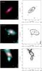 |
Fig. A.1 Left column: the “true color” images, created using the 3.6, 4.5, and 8.0 μm Spitzer/IRAC mosaics, of the 10 galaxies discussed in Sect. 4.3. The images are aligned northeast, and they are 1.5 × 1.5 arcmin in size. Right column: contour maps of the same fields observed in Ks-band with WIRC at the Palomar 5 m telescope. The five contours correspond to 3, 5, 8, 10, and 30σ. Since all images had similar exposure times the noise was σ ~ 19.6 mag arcsec-2. For two galaxies not imaged with WIRC, HCG68a and HCG100a, we used the shallower Ks-band data from 2MASS (σ = 15.7 mag arcsec-2). |
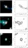 |
Fig. A.1 continued. |
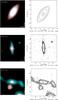 |
Fig. A.1 continued. |
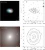 |
Fig. A.1 continued. |
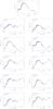 |
Fig. A.2 We display the observed SEDs (blue points) along with the da Cunha model fits (in black) of the 10 peculiar early-type galaxies mentioned in the Appendix. At the top panel we present the SED of a typical field elliptical galaxy, NGC 1404, for comparison. The name of each HCG galaxy is presented along with the χ2 of the model fit to the data. |
The da Cunha et al. (2008) model is publicly available at http://www.iap.fr/magphys
Acknowledgments
T.B., V.C., and T.D.S. would like to acknowledge partial support from the FP7-REGPOT 206469 grant. We would like to thank H. S. Hwang, D. Elbaz, and P.-A. Duc (CEA/Saclay, France) for useful discussions that improved the paper, as well as U. Lisenfeld (Univ. of Granada) for providing the CO data for a number of groups prior to publication.
References
- Aguerri, J. A. L., Castro-Rodríguez, N., Napolitano, N., Arnaboldi, M., & Gerhard, O. 2006, A&A, 457, 771 [NASA ADS] [CrossRef] [EDP Sciences] [Google Scholar]
- Allam, S., Assendorp, R., Longo, G., Braun, M., & Richter, G. 1996, A&AS, 117, 39 [NASA ADS] [CrossRef] [EDP Sciences] [Google Scholar]
- Bahcall, J. N., & Tremaine, S. 1981, ApJ, 244, 805 [NASA ADS] [CrossRef] [Google Scholar]
- Bell, E. F., McIntosh, D. H., Katz, N., & Weinberg, M. D. 2003, ApJS, 149, 289 [NASA ADS] [CrossRef] [Google Scholar]
- Bertin, E. 2008, SWarp, http://astromatic.iap.fr/software/swarp [Google Scholar]
- Bertin, E., & Arnouts, S. 1996, A&AS, 117, 393 [NASA ADS] [CrossRef] [EDP Sciences] [Google Scholar]
- Bitsakis, T., Charmandaris, V., Le Floc’h, E., et al. 2010, A&A, 517, A75 [NASA ADS] [CrossRef] [EDP Sciences] [Google Scholar]
- Bressan, A., Panuzzo, P., Buson, L., et al. 2006, ApJ, 639, L55 [NASA ADS] [CrossRef] [Google Scholar]
- Bicay, M. D., & Giovanelli, R. 1987, ApJ, 321, 645 [NASA ADS] [CrossRef] [Google Scholar]
- Bruzual, G., & Charlot, S. 2003, MNRAS, 344, 1000 [NASA ADS] [CrossRef] [Google Scholar]
- Borthakur, S., Yun, M. S., & Verdes-Montenegro, L. 2010, ApJ, 710, 385 [NASA ADS] [CrossRef] [Google Scholar]
- Buat, V., Iglesias-Páramo, J., Seibert, M., et al. 2005, ApJ, 619, L51 [NASA ADS] [CrossRef] [Google Scholar]
- Calzetti, D., Kennicutt, R. C., Engelbracht, C. W., et al. 2007, ApJ, 666, 870 [NASA ADS] [CrossRef] [Google Scholar]
- Chabrier, G. 2003, PASP, 115, 763 [NASA ADS] [CrossRef] [Google Scholar]
- Charlot, S., & Fall, S. M. 2000, ApJ, 539, 718 [NASA ADS] [CrossRef] [Google Scholar]
- da Cunha, E., Charlot, S., & Elbaz, D. 2008, MNRAS, 388, 1595 [NASA ADS] [CrossRef] [Google Scholar]
- da Cunha, E., Eminian, C., Charlot, S., & Blaizot, J. 2010a, MNRAS, 403, 1894 [NASA ADS] [CrossRef] [Google Scholar]
- da Cunha, E., Charmandaris, V., Díaz-Santos, T., et al. 2010b, A&A, 523, A78 [NASA ADS] [CrossRef] [EDP Sciences] [Google Scholar]
- Dale, D. A., Bendo, G. J., Engelbracht, C. W., et al. 2005, ApJ, 633, 857 [NASA ADS] [CrossRef] [Google Scholar]
- Dale, D. A., Cohen, S. A., Johnson, L. C., et al. 2009, ApJ, 703, 517 [NASA ADS] [CrossRef] [Google Scholar]
- Fazio, G. G., Hora, J. L., Allen, L. E., et al. 2004, ApJS, 154, 10 [NASA ADS] [CrossRef] [Google Scholar]
- Haines, C. P., Gargiulo, A.,La Barbera, F., et al. 2007, MNRAS, 381, 7 [NASA ADS] [CrossRef] [Google Scholar]
- Haines, C. P., Gargiulo, A., & Merluzzi, P. 2008, MNRAS, 385, 1201 [NASA ADS] [CrossRef] [Google Scholar]
- Hernquist, L., Katz, N., & Weinberg, D. H. 1995, ApJ, 442, 57 [NASA ADS] [CrossRef] [Google Scholar]
- Hao, L., Strauss, M. A., Tremonti, C. A., et al. 2005, AJ, 129, 1783 [NASA ADS] [CrossRef] [Google Scholar]
- Hickson, P. 1982, ApJ, 255, 382 [NASA ADS] [CrossRef] [Google Scholar]
- Hickson, P., Kindl, E., & Auman, J. R. 1989, ApJ, 70, 687 [Google Scholar]
- Hickson, P., Mendes de Oliveira, C., Huchra, J. P., & Palumbo, G. G. 1992, ApJ, 399, 353 [NASA ADS] [CrossRef] [EDP Sciences] [MathSciNet] [PubMed] [Google Scholar]
- Hwang, H. S., Elbaz, D., Lee, J. C., et al. 2010, A&A, 522, A33 [NASA ADS] [CrossRef] [EDP Sciences] [Google Scholar]
- Iglesias-Páramo, J., Buat, V., Takeuchi, T. T., et al. 2006, ApJS, 164, 38 [NASA ADS] [CrossRef] [Google Scholar]
- Johnson, K. E., Hibbard, J. E., Gallagher, S. C., et al. 2007, AJ, 134, 1522 [NASA ADS] [CrossRef] [Google Scholar]
- Kaneda, H., Onaka, T., Sakon, I., et al. 2008, ApJ, 684, 270 [NASA ADS] [CrossRef] [MathSciNet] [Google Scholar]
- Kauffmann, G., Heckman, T. M., Tremonti, C., et al. 2003, MNRAS, 346, 1055 [Google Scholar]
- Kennicutt, R. C., Jr., Armus, L., Bendo, G., et al. 2003, PASP, 115, 928 [NASA ADS] [CrossRef] [Google Scholar]
- Kewley, L. J., Groves, B., Kauffmann, G., & Heckman, T. 2006, MNRAS, 372, 961 [NASA ADS] [CrossRef] [Google Scholar]
- Kong, X., Charlot, S., Brinchmann, J., & Fall, S. M. 2004, MNRAS, 349, 769 [NASA ADS] [CrossRef] [Google Scholar]
- Leitherer, C., Schaerer, D., Goldader, J. D., et al. 1999, ApJS, 123, 3 [NASA ADS] [CrossRef] [Google Scholar]
- Mamon, G. A. 1986, ApJ, 307, 426 [NASA ADS] [CrossRef] [Google Scholar]
- Martinez, M. A.,Del Olmo, A., Coziol, R., & Perea, J. 2010, AJ, 139, 1199 [NASA ADS] [CrossRef] [Google Scholar]
- Martinez-Badenes, V., Lisenfeld, U., Espada, D., et al. 2011, A&A, submitted [Google Scholar]
- McConnachie, A. W., Ellison, S. L., & Patton, D. R. 2008, MNRAS, 387, 1281 [NASA ADS] [CrossRef] [Google Scholar]
- Mendes de Oliveira, C., & Hickson, P. 1994, ApJ, 427, 684 [NASA ADS] [CrossRef] [Google Scholar]
- Meurer, G. R., Heckman, T. M., & Calzetti, D. 1999, ApJ, 521, 64 [NASA ADS] [CrossRef] [Google Scholar]
- Morrissey, P., & GALEX Science Team 2005, A&AS, 20717903M [Google Scholar]
- Mulchaey, J. S., Davis, D. S., Mushotzky, R. F., & Burstein, D. 2003, ApJS, 145, 39 [NASA ADS] [CrossRef] [Google Scholar]
- Okada, Y., Murakami, N., Yasuda, A., et al., AKARI FIS Data Users Manual, Version 1.3, http://www.ir.isas.jaxa.jp/ASTRO-F/Observation/ [Google Scholar]
- Panuzzo, P., Rampazzo, R., Bressan, A., et al. 2011, A&A, 528, A10 [NASA ADS] [CrossRef] [EDP Sciences] [Google Scholar]
- Park, C., & Hwang, H. S. 2009, ApJ, 699, 1595 [NASA ADS] [CrossRef] [Google Scholar]
- Ponman, T. J., Bourner, P. D. J., Ebeling, H., & Bohringer, H. 1996, MNRAS, 283, 690 [NASA ADS] [CrossRef] [Google Scholar]
- Rieke, G. H., Young, E. T., Engelbracht, C. W., et al. 2004, ApJS, 154, 25 [NASA ADS] [CrossRef] [Google Scholar]
- Rosenberg, J. L., Wu, Y., Le Floc’h, E., et al. 2008, ApJ, 674, 814 [NASA ADS] [CrossRef] [Google Scholar]
- Salim, S., Rich, R. M., Charlot, S., et al. 2007, ApJS, 173, 267 [NASA ADS] [CrossRef] [Google Scholar]
- Shimada, M., Ohyama, Y., Nishiura, S., Murayama, T., & Taniguchi, Y. 2000, AJ, 119, 2664 [NASA ADS] [CrossRef] [Google Scholar]
- Skrutskie, M. F., Cutri, R. M., Stiening, R., et al. 2006, AJ, 131, 1163 [NASA ADS] [CrossRef] [Google Scholar]
- Slater, S. K., Charmandaris, V., & Haynes, M. P. 2004, BAAS, 36, 728 [NASA ADS] [Google Scholar]
- Smith, B. J., Struck, C., Hancock, M., et al. 2007a, AJ, 133, 791 [NASA ADS] [CrossRef] [Google Scholar]
- Smith, J. D. T., Draine, B. T., Dale, D. A., et al. 2007b, ApJ, 656, 770 [NASA ADS] [CrossRef] [Google Scholar]
- Stern, D., Eisenhardt, P., Gorjian, V., et al. 2005, ApJ, 631, 163 [NASA ADS] [CrossRef] [Google Scholar]
- Strateva, I., Ivezić, Ž., Knapp, G. R., et al. 2001, AJ, 122, 1861 [Google Scholar]
- Struck, C. 1999, Phys. Rep., 321, 1 [NASA ADS] [CrossRef] [Google Scholar]
- Temi, P., Brighenti, F., & Mathews, W. G. 2004, AJ, 633, L25 [Google Scholar]
- Tzanavaris, P., Hornschemeier, A. E., Gallagher, S. C., et al. 2010, ApJ, 716, 556 [NASA ADS] [CrossRef] [Google Scholar]
- Verdes-Montenegro, L., Yun, M. S., Williams, B. A., et al. 2001, A&A, 377, 812 [NASA ADS] [CrossRef] [EDP Sciences] [Google Scholar]
- Véron-Cetty, M.-P., & Véron, P. 2006, A&A, 455, 773 [NASA ADS] [CrossRef] [EDP Sciences] [Google Scholar]
- Walker, L. M., Johnson, K. E., Gallagher, S. C., et al. 2010, Galaxy Wars: Stellar Populations and Star Formation in Interacting Galaxies, 423, 88 [NASA ADS] [Google Scholar]
- Williams, B. A., McMahon, P. M., & van Gorkom, J. H. 1991, AJ, 101, 1957 [NASA ADS] [CrossRef] [Google Scholar]
- Wyder, T., Martin, D. C., Schiminovich, D., et al. 2007, ApJ, 173, 293 [Google Scholar]
- Zibetti, S., Charlot, S., & Rix, H.-W. 2009, MNRAS, 400, 1181 [NASA ADS] [CrossRef] [Google Scholar]
All Tables
The morphological type and derived physical parameters based on the SED modeling of the HCG galaxies.
Derived physical parameters based on the SED modeling of the interacting pair’s galaxy sample.
Distance to, virial radius, and morphology of the nearest neighbor, as well as “strength” of interaction for the HCG galaxies.
Observed and predicted 60 μm and 100 μm IRAS fluxes for each group, as well as total HI, H2, stellar, and dynamical masses.
Properties of the 10 peculiar early-type HCG galaxies and the typical elliptical NGC 1404.
All Figures
|
Fig. 1 Example of best-fit models (in black line) to the observed spectral energy distributions (SEDs) of two galaxies of our sample. One is a typical late-type galaxy (HCG2a; top panel) and the second is a quiescent elliptical galaxy (HCG62a; bottom panel). In each panel, the blue line shows the unattenuated stellar spectrum estimated by the model. The red circles are the observed broadband luminosities with their errors as vertical bars. The residuals, |
| In the text | |
|
Fig. 2 Stellar masses based on the da Cunha et al. (2008) model (hereafter MDCE08) are plotted as a function of the ones derived from Bell et al. (2003) relation based on Ks luminosity (MKs) after applying the corrections discussed in the text. Vertical error bars indicate the 16–84 percentile ranges in the recovered probability distributions, while the horizontal error bars are the 30% errors as described by Bell et al. (2003) determined from the scatter in the models. The blue dashed line represents the one-to-one relation. |
| In the text | |
|
Fig. 3 A plot of the ratio of the SFRs derived from the observed FUV or 24 μm fluxes over the SFRs derived from the da Cunha et al. (2008) model as a function of the model SFR. Red open circles and red open triangles are the SFRs derived from the MIPS 24 μm fluxes for early and the late-type galaxies respectively. Green open circles and green open triangles mark the estimates based on the FUV to IR excess as described by Buat et al. (2005). Filled blue triangles indicate late-type galaxies for which the SFRs are derived from the FUV after estimating the extinction using the β slope method of Meurer et al. (1999). The dashed line is the one-to-one relation. The histogram of the ratios for each method is indicated in the right panel. |
| In the text | |
|
Fig. 4 Histograms of several properties of our HCG sample. Early type galaxies are marked in red and late type galaxies in blue: a) the distributions of the stellar masses (M ∗ ), b) the distributions of the star formation rates (SFR), c) the distributions of specific SFR (sSFR), and d) the histogram of the IR luminosities, LIR, in red, as estimated by our SED modeling. Because of the absence of far-IR observations for most of the sample, we overplot in hashed areas the histograms corresponding to the minimum and maximum LIR of each galaxy, associated to the 16th and 84th percentile ranges of the best fit, respectively, e) a histogram of the extinction inferred from the SED fit (AV, obs) as measured model-derived atttenuated and unattenuated SED (see Sect. 3.1.3). |
| In the text | |
|
Fig. 5 a) Ratio of the intrinsic τV, ISM derived by the model over the observed (attenuated spectrum) τV, obs versus the τV, obs. The dashed line is the one-to-one ratio. The red circles represent the early-type galaxies in HCGs, and the blue diamonds the late-type ones. b) Ratio of the intrinsic τV for stars in birth clouds, derived by the model over the observed τV, obs versus the τV, obs, using the same notation. We excluded 6 galaxies from the plot (HCG44a, HCG47a, HCG47b, HCG56b, HCG59a, and HCG68a) since their χ2 of model-fit was more than 9.00 and the derived τ fairly uncertain (see Table 3). |
| In the text | |
|
Fig. 6 Histograms of the sSFR of the late-type galaxies our three samples, estimated by modeling their SED. The top plot displays in blue the histogram of the sSFR of the 31 late-type galaxies found in dynamically-young, spiral-dominated groups. Overplotted in red is the corresponding histogram of the 42 galaxies in dynamically-old elliptically dominated groups. The middle and bottom plots present the histograms of the 52 late-type galaxies in the Smith et al. (2007a) interacting galaxy pairs, as well as the 71 SINGS late-type galaxies. The arrows indicate the median sSFR value of each distribution. |
| In the text | |
|
Fig. 7 Top panel: IRAC color–color plot of the early-type galaxies in HCGs (black open triangles) and a sample of field ellipticals (blue filled circles). Bottom panel: the histograms of the log[S5.8/S3.6] color of the two samples. The early-type galaxies in the groups are marked with a black line (left axis), while the field ellipticals are presented in blue (right axis). |
| In the text | |
|
Fig. 8 NUV-r histogram of our HCG galaxy sample shown in black (right Y-axis). The histograms of the field, in blue, and cluster galaxies, in red, from the Haines et al. (2008) control sample are also presented (left Y-axis). |
| In the text | |
|
Fig. 9 a) NUV-r histogram of the whole HCG galaxy sample is shown in black. The corresponding histograms of the early- and late-type galaxies of the sample, classified according to their optical morphology, are shown with the red and blue shaded areas. b) The NUV-r distribution of the galaxies hosting an AGN is indicated with the dashed dark line. As above, the early- and late-type hosts are indicated with the red and blue histograms. The region of 3 < NUV-r < 5, identified as “green valley”, is marked with the vertical dashed lines. |
| In the text | |
|
Fig. 10 a) NUV-r histogram of our HCG galaxy sample shown as a black solid line. The corresponding histograms of the early- and late-type galaxies found in dynamically “young” groups are shown with the red and blue shaded areas, respectively. b) Same as in a), but for the galaxies in dynamically “old” groups. The region of 3 < NUV-r < 5, identified as “green valley”, is marked with the vertical dashed lines. |
| In the text | |
|
Fig. 11 A histogram of the NUV-r colors of the HCG sample after correcting for dust extinction, in shown with the black solid line. The separation in two panels for “young” and “old” groups as well as the symbols follow the notation of Fig. 10. |
| In the text | |
|
Fig. 12 The IRAC color–colors plot, originally presented in Fig. 7. Blue circles indicate the spiral galaxies of our HCG sample, blue squares are the irregulars, red triangles are the elliptical galaxies, and red diamonds the lenticular ones. Green dots indicate the LVL galaxies. According to Johnson et al. (2007) the “gap” is located in the area enclosed by the dashed lines. |
| In the text | |
|
Fig. 13 Histograms of the “strength” of the dynamical interaction felt by each group galaxy (⟨ R/rvir, nei ⟩ /n). As usual, we separate our sample into dynamically “young” (blue) and dynamically “old” (red) groups. The arrows indicate the median values of the two distributions. |
| In the text | |
|
Fig. 14 a) Distributions of the total HI masses in the dynamically “young” (in blue) and the dynamically “old” (in red) groups, of the total stellar masses (panel b)) and the total dynamical masses (panel c)). |
| In the text | |
|
Fig. 15 Plot of the ratio of the observed IRAS 60 and 100 μm fluxes of each group divided by the corresponding flux all group members as predicted by our model fits. Since IRAS did not resolve/detect all the members of each group, several of the ratios are indicated as upper limits. Filled symbols indicate dynamically “old” groups. |
| In the text | |
|
Fig. A.1 Left column: the “true color” images, created using the 3.6, 4.5, and 8.0 μm Spitzer/IRAC mosaics, of the 10 galaxies discussed in Sect. 4.3. The images are aligned northeast, and they are 1.5 × 1.5 arcmin in size. Right column: contour maps of the same fields observed in Ks-band with WIRC at the Palomar 5 m telescope. The five contours correspond to 3, 5, 8, 10, and 30σ. Since all images had similar exposure times the noise was σ ~ 19.6 mag arcsec-2. For two galaxies not imaged with WIRC, HCG68a and HCG100a, we used the shallower Ks-band data from 2MASS (σ = 15.7 mag arcsec-2). |
| In the text | |
|
Fig. A.1 continued. |
| In the text | |
|
Fig. A.1 continued. |
| In the text | |
|
Fig. A.1 continued. |
| In the text | |
|
Fig. A.2 We display the observed SEDs (blue points) along with the da Cunha model fits (in black) of the 10 peculiar early-type galaxies mentioned in the Appendix. At the top panel we present the SED of a typical field elliptical galaxy, NGC 1404, for comparison. The name of each HCG galaxy is presented along with the χ2 of the model fit to the data. |
| In the text | |
Current usage metrics show cumulative count of Article Views (full-text article views including HTML views, PDF and ePub downloads, according to the available data) and Abstracts Views on Vision4Press platform.
Data correspond to usage on the plateform after 2015. The current usage metrics is available 48-96 hours after online publication and is updated daily on week days.
Initial download of the metrics may take a while.