| Issue |
A&A
Volume 533, September 2011
|
|
|---|---|---|
| Article Number | A48 | |
| Number of page(s) | 17 | |
| Section | Cosmology (including clusters of galaxies) | |
| DOI | https://doi.org/10.1051/0004-6361/201117236 | |
| Published online | 25 August 2011 | |
Relations between three-point configuration space shear and convergence statistics
1
Argelander-Institut für Astronomie (AIfA), Universität Bonn,
Auf dem Hügel 71,
53121
Bonn,
Germany
e-mail: This email address is being protected from spambots. You need JavaScript enabled to view it.
2 International Max Planck Research School (IMPRS) for
Astronomy and Astrophysics at the Universities of Bonn and Cologne, Germany
3
Institute for Astronomy, University of Edinburgh, Royal
Observatory, Blackford
Hill, Edinburgh,
EH9 3HJ,
UK
Received:
11
May
2011
Accepted:
20
July
2011
Abstract
With the growing interest in and ability of using weak lensing studies to probe the non-Gaussian properties of the matter density field, there is an increasing need for the study of suitable statistical measures, e.g. shear three-point statistics. In this paper we establish the relations between the three-point configuration space shear and convergence statistics, which are an important missing link between different weak lensing three-point statistics and provide an alternative way of relating observation and theory. The method we use also allows us to derive the relations between other two- and three-point correlation functions. We show the consistency of the relations obtained with already established results and demonstrate how they can be evaluated numerically. As a direct application, we use these relations to formulate the condition for E/B-mode decomposition of lensing three-point statistics, which is the basis for constructing new three-point statistics which allow for exact E/B-mode separation. Our work applies also to other two-dimensional polarization fields such as that of the cosmic microwave background.
Key words: gravitational lensing: weak / large-scale structure of Universe / methods: analytical / cosmology: theory
© ESO, 2011
1. Introduction
The statistical study of the weak gravitational lensing effect by the large-scale structure, also called cosmic shear, is one of the established tools to investigate the matter distribution of the Universe and to constrain the parameters of cosmological models. The undergoing boosting of weak lensing survey size and quality gradually enables one to explore the small, non-linear scales where a wealth of signal lies (Bernardeau et al. 2002; Pen et al. 2003; Jarvis et al. 2004; Semboloni et al. 2011). Along with this trend, more and more effort has been put into the development of statistical measures that can probe the non-Gaussian signal arising from the non-linear growth of structure on those scales. Among them, the three-point (3-pt) statistics may be the most widely used.
Two basic quantities considered in gravitational lens theory are the convergence κ and the shear γ. Defined as the dimensionless surface mass density, κ is a weighted projection of the three-dimensional (3D) matter density contrast δ. The shear γ, on the other hand, is directly accessible from observations. Therefore, the theoretical framework of gravitational lensing should include the relation between configuration space κ and γ statistics as well as the one relating configuration space statistics to their Fourier space counterparts. At the level of two-point (2-pt) statistics, such relations have already been established. For 3-pt statistics, the relation between the shear 3-pt correlation functions (γ3PCFs) and the convergence bispectrum, which is the Fourier counterpart of the 3-pt convergence correlation function (κ3PCF), has been derived by Schneider et al. (2005). The other non-trivial relation, the one between γ3PCFs and κ3PCFs, is still missing. One purpose of this work is to establish this missing link.
How to perform E/B-mode decomposition is also a major concern of the weak lensing community. For observational data an E/B-mode decomposition provides a necessary check on the possible systematics (e.g. Crittenden et al. 2002; Pen et al. 2002). In recent years there have been several efforts to construct better statistics which allow for an E/B-mode decomposition at the 2-pt level (Schneider & Kilbinger 2007; Eifler et al. 2010; Fu & Kilbinger 2010; Schneider et al. 2010). They all use weight functions to filter the shear 2-pt correlation functions (γ2PCFs), and the condition for E/B-mode decomposition transforms to a condition on the weight functions. Such a condition at the 3-pt level is also missing so far. We will see that with the aid of the relation between the γ3PCFs and the κ3PCFs, one can easily formulate this condition.
The paper is organized as follows: In Sect. 2 we show how the relation between the γ3PCF and the κ3PCF is obtained. In Sect. 3 we investigate the correspondence between the derived relation and already established results. We then extend our results to other γ3PCFs in Sect. 4, and in Sect. 5 we present an application of the 3-pt relations, deriving the condition for E/B-mode separation of 3-pt shear statistics. How these relations can be numerically evaluated is demonstrated in Sect. 6, and we conclude in Sect. 7.
2. Relation between 3-pt γ and κ correlation functions
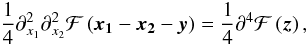
2.1. The form of the relation
At the 2-pt level, the relation between the configuration space shear and convergence
statistics is the ξ+ − ξ−
relation (Crittenden et al. 2002; Schneider et al. 2002) 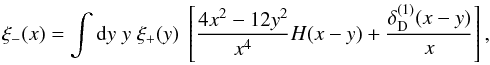 (1)where H
and
(1)where H
and  are Heaviside function and 1D Dirac delta function, respectively. The functions
ξ+ and ξ− are defined as
ξ+(x): = ⟨ κκ ⟩ (|x|)
and
ξ−(x): = ⟨ γγ ⟩ (x) e−4iφx,
with φx being the polar angle of the
separation vector x, and ⟨ ⟩ indicating the ensemble
average. Note that the shear γ is a spin-2 quantity, i.e. it gets
multiplied by a phase factor
e−2iφx when the coordinate
x rotates by
φx. Consequently,
⟨ γγ ⟩ (x) has a spin of 4. Being the
product of ⟨ γγ ⟩ (x) and a phase factor
of e−4iφx, the quantity
ξ−(x) no longer depends on the polar
angle of x.
are Heaviside function and 1D Dirac delta function, respectively. The functions
ξ+ and ξ− are defined as
ξ+(x): = ⟨ κκ ⟩ (|x|)
and
ξ−(x): = ⟨ γγ ⟩ (x) e−4iφx,
with φx being the polar angle of the
separation vector x, and ⟨ ⟩ indicating the ensemble
average. Note that the shear γ is a spin-2 quantity, i.e. it gets
multiplied by a phase factor
e−2iφx when the coordinate
x rotates by
φx. Consequently,
⟨ γγ ⟩ (x) has a spin of 4. Being the
product of ⟨ γγ ⟩ (x) and a phase factor
of e−4iφx, the quantity
ξ−(x) no longer depends on the polar
angle of x.
The relation (1) has already taken both
the statistical homogeneity and isotropy of the shear field into account and is therefore
a one-dimensional relation of quantities on the real domain. The derivation of the
ξ+−ξ− relation originates
from the relation between ξ+ and
ξ− and the convergence power spectrum
Pκ,  (2)Inverting one of the
relations in (2) one can write
ξ+ and ξ− in terms of each
other, e.g.
(2)Inverting one of the
relations in (2) one can write
ξ+ and ξ− in terms of each
other, e.g.  (3)and the final form
of the relation (1) can be reached by
performing the 1D Bessel integral whose result can be obtained from Gradshteyn et al. (2000).
(3)and the final form
of the relation (1) can be reached by
performing the 1D Bessel integral whose result can be obtained from Gradshteyn et al. (2000).
The same procedure, however, fails to work for 3-pt statistics since the corresponding Bessel integral actually consists of three integrals, and they have highly complicated dependencies on the arguments (see Schneider et al. 2005). A brute force numerical evaluation of these integrals is also extremely challenging due to the oscillatory behaviour of the Bessel functions.
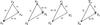 |
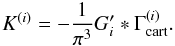
Fig. 1 Definition of the geometry of a triangle (the leftmost sketch) and how it changes under permutations (the first three sketches from the left) and flip (the leftmost and the rightmost sketch) of the vertices. |
Since the advantage of transforming to the Fourier plane and back no longer holds for 3-pt statistics, we attempt to stay in configuration space, which at least avoids the problem of oscillatory integrals. One can see from (1) that the result of the Bessel integral in (3) is actually not oscillatory, as expected.
The configuration space 3-pt shear correlator can be written as
⟨γ(X1)γ(X2)γ(X3)⟩,
with Xi being the
positions on the two-dimensional (2D) plane where the shear signals are evaluated.
Following the assumed statistical homogeneity of the shear field, the correlator depends
only on the separations of these three positions. We choose
x1 ≡ X1 − X3
and
x2 ≡ X2 − X3
to be its arguments (see the leftmost sketch of Fig. 1) and write the correlator as
⟨ γγγ ⟩ (x1,x2).
After the same procedure is applied to the 3-pt convergence correlator, the relation we
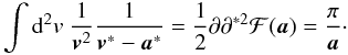
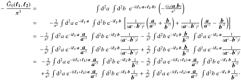
are interested in will be shown to be of the form  (4)where we have defined
the convolution kernel G0 for which we need to find an
explicit expression.
(4)where we have defined
the convolution kernel G0 for which we need to find an
explicit expression.
Writing the relation in the form of a convolution is motivated by the Kaiser-Squires
(K-S) relation between the convergence and the shear (Kaiser & Squires 1993),  (5)which yields the
result (4) and also allows us to express
the kernel G0 as
(5)which yields the
result (4) and also allows us to express
the kernel G0 as  (6)Here, for simplicity, we
have adopted the complex notation for the K-S kernel, i.e. we have identified the 2D
separation vectors with complex numbers. Throughout the text we will use the vector and
complex notations interchangeably, and use x to indicate a
complex quantity, x for its absolute value, and
x∗ for its complex conjugate.
(6)Here, for simplicity, we
have adopted the complex notation for the K-S kernel, i.e. we have identified the 2D
separation vectors with complex numbers. Throughout the text we will use the vector and
complex notations interchangeably, and use x to indicate a
complex quantity, x for its absolute value, and
x∗ for its complex conjugate.
The integral in (6) is difficult to
perform directly, so we first take a look at the more studied 2-pt case. The relation
between 2-pt γ and κ correlation functions can be
written in the same way as 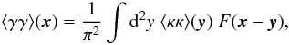 (7)with
 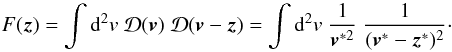 (8)Unlike the case of the
ξ+ − ξ− relation, we have
not assumed a statistically isotropic field for (4) or (7). The
ξ+ − ξ− relation is actually
what one should obtain after adding the assumption of isotropy to (7).
(8)Unlike the case of the
ξ+ − ξ− relation, we have
not assumed a statistically isotropic field for (4) or (7). The
ξ+ − ξ− relation is actually
what one should obtain after adding the assumption of isotropy to (7).
2.2. The form of the convolution kernels
Now we aim for obtaining the forms of the F and
G0 kernels, which can be seen as the 2- and 3-pt equivalence
of the K-S kernel (5). Introducing the
symbols
∂ ≡ ∂1 + i∂2
and  , the definitions of
κ and γ read
, the definitions of
κ and γ read 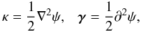 (9)i.e. both the
convergence κ and the shear γ are
second-order derivatives of the deflection potential ψ. It is then
convenient to use ψ as a link between κ and
γ. Using the identities
∇ln|x| = x/|x|2
and
(9)i.e. both the
convergence κ and the shear γ are
second-order derivatives of the deflection potential ψ. It is then
convenient to use ψ as a link between κ and
γ. Using the identities
∇ln|x| = x/|x|2
and 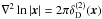 which hold for a 2D
x, one can easily verify the consistency of (9) with the relation between ψ
and κ (e.g. Bartelmann & Schneider
2001),
which hold for a 2D
x, one can easily verify the consistency of (9) with the relation between ψ
and κ (e.g. Bartelmann & Schneider
2001), 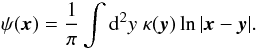 (10)Applying the operator
∂2 on both sides of (10) and taking (9) into
account, one reaches the K-S relation (5),
since
(10)Applying the operator
∂2 on both sides of (10) and taking (9) into
account, one reaches the K-S relation (5),
since  ∂2ln|z|.
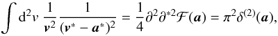
The same procedure can be generalized to second-order statistics. The 2-pt equivalence
of (10) is  (11)Using the
statistical homogeneity of the κ field, and re-defining the integration
variables, (11) reduces to
(11)Using the
statistical homogeneity of the κ field, and re-defining the integration
variables, (11) reduces to 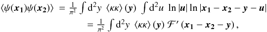 (12)where
we have defined
(12)where
we have defined 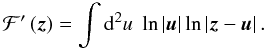 (13)Obviously, ℱ′ is
infinite at every z, which is related to the fact that
ψ is defined only up to an additive constant. However, we shall only
need the derivatives of ℱ′. So we define
(13)Obviously, ℱ′ is
infinite at every z, which is related to the fact that
ψ is defined only up to an additive constant. However, we shall only
need the derivatives of ℱ′. So we define 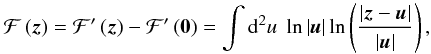 (14)and will use ℱ and ℱ′
interchangeably. Let ϕ denote the angle between
u and z, (14) can be rewritten as
(14)and will use ℱ and ℱ′
interchangeably. Let ϕ denote the angle between
u and z, (14) can be rewritten as
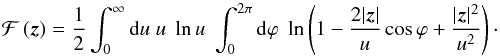 (15)The integral over
ϕ yields zero if
|z| < u, and
4πln(|z|/u)
otherwise. Thus
(15)The integral over
ϕ yields zero if
|z| < u, and
4πln(|z|/u)
otherwise. Thus 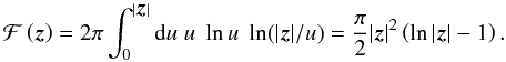 (16)We are now ready to
apply differential operators to (12) to
get the relations of 2-pt shear and convergence statistics. As a consistency check, we
first apply two ∇2 operators to (12), one acting on
x1 and the other on
x2. According
to (9), this turns the l.h.s. of (12) into
4⟨κ(x1)κ(x2)⟩.
On the r.h.s. of (12) the operators act
exclusively on ℱ,
(16)We are now ready to
apply differential operators to (12) to
get the relations of 2-pt shear and convergence statistics. As a consistency check, we
first apply two ∇2 operators to (12), one acting on
x1 and the other on
x2. According
to (9), this turns the l.h.s. of (12) into
4⟨κ(x1)κ(x2)⟩.
On the r.h.s. of (12) the operators act
exclusively on ℱ,  (17)with
z = x1 − x2 − y
here. Using (17), one easily sees that the
r.h.s. of (12) after the operation gives
4⟨κκ⟩(x1 − x2),
which is equivalent to
4⟨κ(x1)κ(x2)⟩
under the assumption of statistical homogeneity of the κ field. Now we
apply the operator
(17)with
z = x1 − x2 − y
here. Using (17), one easily sees that the
r.h.s. of (12) after the operation gives
4⟨κκ⟩(x1 − x2),
which is equivalent to
4⟨κ(x1)κ(x2)⟩
under the assumption of statistical homogeneity of the κ field. Now we
apply the operator  on (12), which turns the l.h.s.
of (12) into
⟨γ(x1)γ(x2)⟩.
On the r.h.s. the operation again acts only on ℱ,
on (12), which turns the l.h.s.
of (12) into
⟨γ(x1)γ(x2)⟩.
On the r.h.s. the operation again acts only on ℱ,
 (18)also with
z = x1 − x2 − y.
Remembering the definition of the kernel F (7), this leads to
(18)also with
z = x1 − x2 − y.
Remembering the definition of the kernel F (7), this leads to 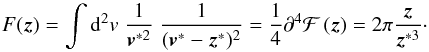 (19)For the 3-pt kernel
G0 we split the integral in (6) into
(19)For the 3-pt kernel
G0 we split the integral in (6) into 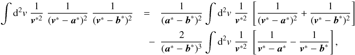 (20)where
we have assumed a ≠ b.
From (19) as well as
(20)where
we have assumed a ≠ b.
From (19) as well as
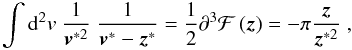 (21)we obtain
  (22)The forms of the
kernels (19) and (22) hold rigorously outside their
singularities (at z = 0 for F; at
a = 0, b = 0, and
a = b for
G0). One may wonder if additional delta functions exist at
these singularities. We will show in Sect. 3 that
this is not the case.
(22)The forms of the
kernels (19) and (22) hold rigorously outside their
singularities (at z = 0 for F; at
a = 0, b = 0, and
a = b for
G0). One may wonder if additional delta functions exist at
these singularities. We will show in Sect. 3 that
this is not the case.
The method we used to derive the forms of the kernels (19) and (22) also allows one to derive the relations between other correlation functions of weak lensing quantities in a systematic way. We present explicit forms of some of the relations in Appendix B.
2.3. The relations
To summarize, we have obtained: 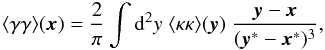 (23)and
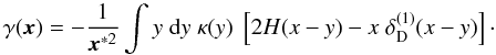
 ![Mathematical equation: \begin{eqnarray} \label{eq:Grelation} \langle \gamma\gamma\gamma \rangle(\vek{x_1},\vek{x_2})& = -\frac{2}{\pi^2}\;\int \dd^2 y_1 \int \dd^2 y_2\; \langle \kappa\kappa\kappa \rangle (\vek{y_1},\vek{y_2}) \; \Bigg[ \frac{1}{{(\vek{y_1}^*-\vek{x_1}^*-\vek{y_2}^*+\vek{x_2}^*)^2}} \br{\frac{\vek{y_1}-\vek{x_1}}{(\vek{y_1}^*-\vek{x_1}^*)^{3}}+\frac{\vek{y_2}-\vek{x_2}}{(\vek{y_2}^*-\vek{x_2}^*)^{3}}}\nonumber\\ & + \frac{1}{(\vek{y_1}^*-\vek{x_1}^*-\vek{y_2}^*+\vek{x_2}^*)^3}\br{\frac{\vek{y_1}-\vek{x_1}}{(\vek{y_1}^*-\vek{x_1}^*)^{2}}-\frac{\vek{y_2}-\vek{x_2}}{(\vek{y_2}^*-\vek{x_2}^*)^{2}}} \Bigg]\cdot \end{eqnarray}](/articles/aa/full_html/2011/09/aa17236-11/aa17236-11-eq80.png) (24)In
these relations we have applied the statistical homogeneity of the convergence field, but
not the statistical isotropy. Making use of the latter, one can derive the
ξ+ − ξ− relation from (23), as will be shown in Sect. 3.2.
(24)In
these relations we have applied the statistical homogeneity of the convergence field, but
not the statistical isotropy. Making use of the latter, one can derive the
ξ+ − ξ− relation from (23), as will be shown in Sect. 3.2.
3. Consistency checks
3.1. The case of uniform κ
There is a physical condition which will directly serve as a test of the κ − γ relations (5), (23) and (24). At the 1-pt level, for the K-S relation, a uniform convergence field does not result in any shear. At the 2- and 3-pt level, the physical condition could be that a uniform ⟨ κκ ⟩ (⟨ κκκ ⟩ ) field leads to a vanishing shear correlation ⟨ γγ ⟩ (⟨ γγγ ⟩ ).
One can easily see that both the F and G0 kernel we obtained satisfy this condition. If there are additional terms at the singularities of the kernels which contribute to the integral, a non-zero ⟨ γγ ⟩ (⟨ γγγ ⟩ ) term would be generated and the condition would not be satisfied anymore. Thus we argue that the expressions (23) and (24) are already complete.
3.2. Consistency with the ξ+ − ξ− relation
Now we consider whether (23) is
consistent with the ξ+ − ξ−
relation (1), which can be regarded as
the isotropic form of (23). That the two
relations are consistent is equivalent to 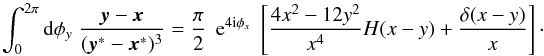 (25)To verify that (25) indeed holds, we attempt to solve the
φy-integral on the l.h.s.,
(25)To verify that (25) indeed holds, we attempt to solve the
φy-integral on the l.h.s., 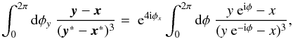 (26)where
φ = φy − φx
has been defined. The φ-integral can be carried out using the residual
theorem, yielding
2π(x2 − 3y2)/x4
when x > y and zero when
x < y. One can see that this result corresponds
to the Heaviside function on the r.h.s. of (25).
(26)where
φ = φy − φx
has been defined. The φ-integral can be carried out using the residual
theorem, yielding
2π(x2 − 3y2)/x4
when x > y and zero when
x < y. One can see that this result corresponds
to the Heaviside function on the r.h.s. of (25).
At the singularity x = y the φ-integral is not well defined, which means one cannot rule out the existence of additional delta function at x = y in the result of the φ-integral. This ambiguity can again be eliminated by using the physical condition “a uniform ⟨ κκ ⟩ field leads to a null shear correlation ⟨ γγ ⟩ ”, which translates to “a constant ξ+ yields vanishing ξ−” here. In this case, a delta function is indeed required to satisfy this condition, and the prefactor of the delta function can be determined to be π/2x, in consistency with (25).
3.2.1. K-S relation and its isotropic form
A similar consistency exists between the K-S relation and its isotropic form. As both forms are already well-known, they can serve as a further support for our argument.
For an axisymmetric distribution of matter, i.e.
κ(x) = κ(x),
the following relation is established between the shear and the convergence (see e.g.
Schneider et al. 1992)
 (27)with
 defined as
 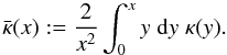 (28)This is equivalent to
 (29)In the case of a
uniform convergence field κ(x) = const., one can see
that the integral of the Heaviside function and the delta function parts cancel each
other.
(29)In the case of a
uniform convergence field κ(x) = const., one can see
that the integral of the Heaviside function and the delta function parts cancel each
other.
The similarity between (29) and the ξ+ − ξ− relation (1) is remarkable: they both have integrals of a Heaviside function part and a delta function part which cancel each other for constant κ and ⟨κκ⟩, respectively, and the 2D correspondences of both do not have an additional delta function at their singularities.
3.3. Fourier transformations
In the Fourier plane the relation between the shear and the convergence has a simple
form. With  denoting the Fourier transformation of the quantity g, it
reads
denoting the Fourier transformation of the quantity g, it
reads  (30)with
β being the polar angle of the wave vector
ℓ. The identity (30) can be obtained by relating the Fourier transforms of the definitions (9) of γ and
κ. It directly reflects the fact that γ is spin-2 while
κ is spin-0, and leads to the well-known result
Pγ = Pκ.
Comparing (30) to the configuration
space relation (5) which means
(30)with
β being the polar angle of the wave vector
ℓ. The identity (30) can be obtained by relating the Fourier transforms of the definitions (9) of γ and
κ. It directly reflects the fact that γ is spin-2 while
κ is spin-0, and leads to the well-known result
Pγ = Pκ.
Comparing (30) to the configuration
space relation (5) which means
 ,
using the convolution theorem, one can see that
,
using the convolution theorem, one can see that  for
ℓ ≠ 0.
for
ℓ ≠ 0.
The Fourier plane correspondences of (23)
and (24) are also readily obtainable
from the identity (30), as  (31)and
  (32)with
βi denoting the polar angle of
ℓi. These
equations show that
(32)with
βi denoting the polar angle of
ℓi. These
equations show that  for
ℓ ≠ 0, and that
for
ℓ ≠ 0, and that
 for
ℓ1 ≠ 0 ≠ ℓ2
and
ℓ3 = −ℓ1 − ℓ2 ≠ 0,
since F/π2 and
−G0/π3 are the convolution
kernels for the configuration space relations by their definitions.
for
ℓ1 ≠ 0 ≠ ℓ2
and
ℓ3 = −ℓ1 − ℓ2 ≠ 0,
since F/π2 and
−G0/π3 are the convolution
kernels for the configuration space relations by their definitions.
In Appendix A we show explicitly that the Fourier
transforms of F/π2 and
−G0/π3, with
F and G0 given in (19) and (22), are indeed e4iβ and
e2i(β1 + β2 + β3),
respectively. However one cannot obtain the forms of F and
G0 kernels simply through inverse Fourier transforming the
phase factors e4iβ and
e2i(β1 + β2 + β3).
This is due to the fact that the Fourier inversion theorem is valid strictly only for
square-integrable functions, which is not the case for the phase factors. The same
situation occurs for the K-S kernel  .
.
4. The other γ3PCFs
Until now we have considered only the 3PCF of shear itself
⟨γ(X1)γ(X2)γ(X3)⟩,
which is one of the four independent possible combinations considering that
γ is a complex quantity. The other three are
⟨γ∗(X1)γ(X2)γ(X3)⟩,
⟨γ(X1)γ∗(X2)γ(X3)⟩,
and
⟨γ(X1)γ(X2)γ∗(X3)⟩,
according to the choice made in Schneider & Lombardi
(2003). Following Schneider et al. (2005),
we denote these four γ3PCFs by  (i = 0,1,2,3), with ‘cart’ emphasizing that the shear is measured in
Cartesian coordinates,
(i = 0,1,2,3), with ‘cart’ emphasizing that the shear is measured in
Cartesian coordinates,  , and
, and
 (i = 1,2,3) corresponding to the γ3PCF with
γ∗ at position
Xi. Since we
have considered statistical homogeneity of the shear field, the Γcart’s depend
only on the separation vectors of the position X1,
X2, and X3. The other
γ3PCFs, i.e. those with two or three γ∗’s,
can be obtained by taking the complex conjugate of the Γcart’s.
(i = 1,2,3) corresponding to the γ3PCF with
γ∗ at position
Xi. Since we
have considered statistical homogeneity of the shear field, the Γcart’s depend
only on the separation vectors of the position X1,
X2, and X3. The other
γ3PCFs, i.e. those with two or three γ∗’s,
can be obtained by taking the complex conjugate of the Γcart’s.
Note that 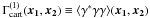 ,
,
 , and
, and
 are different functions,
since x1
(x2) is defined to be the difference of the positions of the
first (second) and the third γ in the bracket. Due to the same reason, they
can be transformed into each other through permutations and flips of the vertices of the
triangle formed by their arguments (see Fig. 1), and
thus are not independent if argument permutations and flips are allowed. As an example, one
has
are different functions,
since x1
(x2) is defined to be the difference of the positions of the
first (second) and the third γ in the bracket. Due to the same reason, they
can be transformed into each other through permutations and flips of the vertices of the
triangle formed by their arguments (see Fig. 1), and
thus are not independent if argument permutations and flips are allowed. As an example, one
has  (33)where
different lines correspond to different ways of labeling the same triangle with side lengths
x1, x2, and
|x1 − x2|.
The same permutations and flips also reveal the inherent symmetry of
(33)where
different lines correspond to different ways of labeling the same triangle with side lengths
x1, x2, and
|x1 − x2|.
The same permutations and flips also reveal the inherent symmetry of
 ,
,
 (34)In the case that the
shear is measured relative to a center of the triangle,
transforms to Γ(i), the natural components of the
γ3PCF as defined in Schneider &
Lombardi (2003). For a general triangle configuration, all four Γcart’s
are expected to be non-zero, thus all of them should be used to exploit the full 3-pt
information of cosmic shear.
(34)In the case that the
shear is measured relative to a center of the triangle,
transforms to Γ(i), the natural components of the
γ3PCF as defined in Schneider &
Lombardi (2003). For a general triangle configuration, all four Γcart’s
are expected to be non-zero, thus all of them should be used to exploit the full 3-pt
information of cosmic shear.
Before relating the other Γcart’s to the κ3PCFs, we extend
κ to a complex quantity
κ = κE + iκB.
Although the physical convergence is a real quantity, the convergence field corresponding to
the measured shear signals can have an imaginary part due to e.g. systematical errors and
noise. The shear component which corresponds to this unphysical imaginary part of the
convergence field is identified as the B-mode, on which we will elaborate more in
Sect. 6. When taking the B-mode into consideration,
the 3-pt correlation functions of the convergence field can be written as 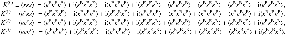 (35)Apart
from the E-mode
⟨ κEκEκE ⟩
term, there are still additional B-mode contributions to the real parts of the
K’s, namely
⟨ κEκBκB ⟩ ,
⟨ κBκEκB ⟩ ,
and
⟨ κBκBκE ⟩ .
The imaginary part of the K’s are composed of the parity violating terms
which are expected to vanish due to parity symmetry (Schneider 2003). The property of K(i)
under permutations and flips of the vertices of the triangle formed by their arguments is
the same as that of .
(35)Apart
from the E-mode
⟨ κEκEκE ⟩
term, there are still additional B-mode contributions to the real parts of the
K’s, namely
⟨ κEκBκB ⟩ ,
⟨ κBκEκB ⟩ ,
and
⟨ κBκBκE ⟩ .
The imaginary part of the K’s are composed of the parity violating terms
which are expected to vanish due to parity symmetry (Schneider 2003). The property of K(i)
under permutations and flips of the vertices of the triangle formed by their arguments is
the same as that of .
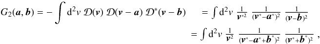
Similar to (4), the relations between
and K(i) for i = 1,2,3 can be
written as  (36)
(36) (37)and
  (38)where the convolution
kernels G1, G2, and
G3 have been defined. Again with the aid of the K-S relation,
we can write these convolution kernels as
(38)where the convolution
kernels G1, G2, and
G3 have been defined. Again with the aid of the K-S relation,
we can write these convolution kernels as 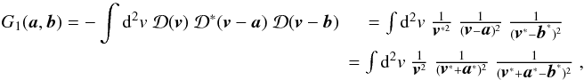 (39)
(39) (40)and
 (41)When
a ≠ b, the product of the
three terms in the integrand of (41) can be
split into products of two, as
(41)When
a ≠ b, the product of the
three terms in the integrand of (41) can be
split into products of two, as  (42)These terms are also
obtainable from doing derivatives to the kernel ℱ,
(42)These terms are also
obtainable from doing derivatives to the kernel ℱ,
 (43)
(43) (44)This way we obtain
the form of the convolution kernel G3. The forms for the kernel
G1 and G2 can be obtained
likewise. The results are
(44)This way we obtain
the form of the convolution kernel G3. The forms for the kernel
G1 and G2 can be obtained
likewise. The results are  (45)
(45)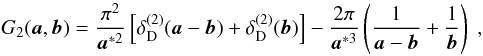 (46)
(46)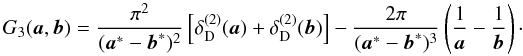 (47)The symmetries in the
Γcart’s and K’s are also reflected in the G
kernels. One can verify that
G2(a,b) = G1(b − a, −a),
G3(a,b) = G1(−b,a − b)
as results of the symmetry under permutations, and
G2(a,b) = G1(b,a),
G3(a,b) = G3(b,a)
as results of the symmetry under flips, in consistency with (33). Similarly, one has
G0(a, b) = G0(b − a, −a) = G0(−b,a − b) = G0(b, a),
in consistency with (34).
(47)The symmetries in the
Γcart’s and K’s are also reflected in the G
kernels. One can verify that
G2(a,b) = G1(b − a, −a),
G3(a,b) = G1(−b,a − b)
as results of the symmetry under permutations, and
G2(a,b) = G1(b,a),
G3(a,b) = G3(b,a)
as results of the symmetry under flips, in consistency with (33). Similarly, one has
G0(a, b) = G0(b − a, −a) = G0(−b,a − b) = G0(b, a),
in consistency with (34).
5. Inverse relations
So far we have obtained the expressions of the four γ3PCFs as functions of
the κ3PCFs. Written in a short form, they are 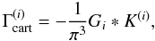 (48)where
i runs from 0 to 3. The forms of the
Gi kernels are given by (22), (45), (46), and (47).
(48)where
i runs from 0 to 3. The forms of the
Gi kernels are given by (22), (45), (46), and (47).
These relations can be inverted. We define the kernels of the inverse relations to be
 , i.e.
 (49)Using the convolution
theorem, it is apparent from (48) and (49) that
(49)Using the convolution
theorem, it is apparent from (48) and (49) that 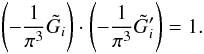 (50)From the corresponding
Fourier plane relations of (48), we also
know
(50)From the corresponding
Fourier plane relations of (48), we also
know  (51)which implies
  (52)Comparing (50) and (52) one has
  (53)and further,
 (54)i.e. the convolution
kernel for the inverse relation is the complex conjugate of the original kernel.
(54)i.e. the convolution
kernel for the inverse relation is the complex conjugate of the original kernel.
This property of the convolution kernel has its root in the fact that
 and
and
 differ only by a phase factor. This fact also endows the convolution kernels in the 1-pt and
2-pt relations between γ and κ with the same property. As
is well known for the 1-pt relation, the inverse relation of (5) is
differ only by a phase factor. This fact also endows the convolution kernels in the 1-pt and
2-pt relations between γ and κ with the same property. As
is well known for the 1-pt relation, the inverse relation of (5) is 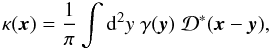 (55)where the kernel is the
complex conjugate of the K-S kernel .
The inverse relation of the 2-pt relation (7)
can also be shown to be
(55)where the kernel is the
complex conjugate of the K-S kernel .
The inverse relation of the 2-pt relation (7)
can also be shown to be 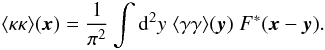 (56)
(56)
6. Condition of 3pt E/B decomposition
Being mathematically a polarization field, the shear field can be decomposed into a curl-free component and a divergence-free component, usually called the E-mode and the B-mode, respectively. Performing such a decomposition when treating cosmic shear data has long been recognized as a necessity, since it provides a valuable check on the possible systematics (e.g. Crittenden et al. 2002; Pen et al. 2002).
The E/B-mode decomposition can be done either on the shear field itself (e.g. Bunn et al. 2003; Bunn 2011), or at the level of correlation functions (e.g. Schneider 2006). The complex survey geometry after masking, which is especially characteristic for a lensing survey (e.g. Erben et al. 2009), renders the first option barely feasible, and singles out the correlation function as the basic statistic to be applied directly to the data. Thus the natural way to perform the E/B-mode decomposition on cosmic shear data is to derive statistics based on the shear correlation functions.
A commonly used statistic for this purpose is the aperture mass statistic which can be
expressed as a linear combination of ξ+ and
ξ− (Schneider et al.
2002), 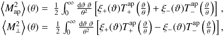 (57)where
the forms of the weight functions
(57)where
the forms of the weight functions  and
and
 are given explicitly
in Schneider et al. (2002). The chosen forms of the
weight functions guarantee that
are given explicitly
in Schneider et al. (2002). The chosen forms of the
weight functions guarantee that  responds only to the E-mode and
  only to the B-mode.
The aperture mass statistics has been generalized to 3-pt level by Jarvis et al. (2004) and Kilbinger & Schneider (2005), and is the only statistics available up to now which allows an E/B-mode decomposition at the 3-pt level. However, as found by Kilbinger et al. (2006), it cannot ensure a clean E/B-mode decomposition when applied to real data. The lack of shear-correlation measurements on small and large scales, which arises from the inability of shape measurement for close projected galaxy pairs and the finite field size, prohibits one from performing the integral in (57) from zero to infinity, and thus introduces a mixing of the E- and B-modes.
In recent years, there have been several efforts to construct better statistics which allow
E/B-mode decomposition (Schneider & Kilbinger
2007; Eifler et al. 2010; Fu & Kilbinger 2010; Schneider et al. 2010), all of them focusing on the cosmic shear 2-pt
statistics. These new statistics are based on the idea that the weight functions
and
used in the aperture
mass statistics are just one example out of the many possibilities. In general one can
define second-order statistics in the form (Schneider
& Kilbinger 2007) 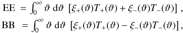 (58)for
which the condition that EE responds only to E-mode and BB only to B-mode is found to be
(58)for
which the condition that EE responds only to E-mode and BB only to B-mode is found to be
 (59)Note
that instead of being functions of the separation length as the aperture mass statistics, EE
and BB are just numbers. At first sight one seems to have reduced the information quantity
by integrating over the scale dependence in (58). In fact, the information can be easily regained by constructing a set of
weight functions satisfying (59). As one
example,
(59)Note
that instead of being functions of the separation length as the aperture mass statistics, EE
and BB are just numbers. At first sight one seems to have reduced the information quantity
by integrating over the scale dependence in (58). In fact, the information can be easily regained by constructing a set of
weight functions satisfying (59). As one
example,  and
and
 for any
θ value can be reconstructed in the framework of (58) by specifying
for any
θ value can be reconstructed in the framework of (58) by specifying
 and
and
 .
.
Since the condition for E/B-mode decomposition (59) still leaves large freedom for the choice of the weight functions, one can
construct statistics which fulfill additional constraints, e.g. a finite support over the
separation length. If one requires that EE and BB respond only to
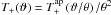
ξ+(ϑ) and
ξ−(ϑ) with
ϑmin < ϑ < ϑmax,
where ϑmin and ϑmax are the chosen
small- and large-scale cutoff, T+(ϑ) and
T−(ϑ) must vanish outside the same range.
Since T+ and T− are interrelated
by (59), one can specify only one of them
to satisfy this constraint. The requirement that the other weight function also vanishes
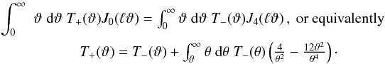
outside the specified range needs to be put as additional integral constraints. As shown by
Schneider & Kilbinger (2007), if one
chooses T− to vanish for
ϑ < ϑmin and
ϑ > ϑmax, then to allow an E/B-mode
decomposition on a finite interval
ϑmin < ϑ < ϑmax,
T− has to satisfy additionally,  (60)which would guarantee that
T+ vanishes for
ϑ < ϑmin and
ϑ > ϑmax.
(60)which would guarantee that
T+ vanishes for
ϑ < ϑmin and
ϑ > ϑmax.
Similar statistics are needed at the 3-pt level as well. The first step required is to formulate the conditions for 3-pt weight functions to allow E/B-mode decomposition, in analogy to (59). As we will show in this section, the relations between the γ3PCFs and κ3PCFs that we derived provide a natural way of formulating such conditions.
A pure E-mode shear 3-pt statistics is related only to the E-mode κ3PCF
⟨ κEκEκE ⟩
but not to other 3PCFs with κB contribution. Therefore we first
write the 3PCFs of κE and κB as
linear combinations of the real and imaginary parts of the
K(i)’s, using (35), and then relate them with the
Γcart’s through (49), as the
Γcart’s are the directly measurable statistics from a lensing survey. The
results read 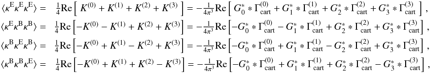 (61)and
 (62)which
shows how the E- and B-mode κ3PCFs can be computed when the full
information of the Γcart’s is available. In the ideal case that there exists no
noise or systematical effects, only the E-mode term κ3PCF
⟨ κEκEκE ⟩
is expected to be non-zero, since it corresponds to the correlation in the physical density
field which leads to the correlation in the shear signal.
(62)which
shows how the E- and B-mode κ3PCFs can be computed when the full
information of the Γcart’s is available. In the ideal case that there exists no
noise or systematical effects, only the E-mode term κ3PCF
⟨ κEκEκE ⟩
is expected to be non-zero, since it corresponds to the correlation in the physical density
field which leads to the correlation in the shear signal.
Following the ideas of Schneider & Kilbinger
(2007), we construct a new statistic 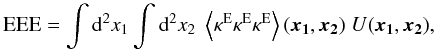 (63)which by definition
responds only to E-mode. With the help of (61) we can link EEE to the observable Γcart’s, as
(63)which by definition
responds only to E-mode. With the help of (61) we can link EEE to the observable Γcart’s, as 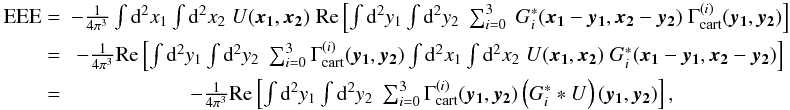 (64)where
in the first equation we have specified U to be a real function, and in the
second equation we have used the fact that
Gi(−a, −b) = Gi(a,b).
(64)where
in the first equation we have specified U to be a real function, and in the
second equation we have used the fact that
Gi(−a, −b) = Gi(a,b).
Denoting 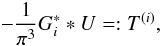 (65)the expression of
EEE (64) has a similar form as (58). We can see in this form that EEE responds
only to the E-mode if the weight function T’s satisfy
(65)the expression of
EEE (64) has a similar form as (58). We can see in this form that EEE responds
only to the E-mode if the weight function T’s satisfy  (66)with
U being a real function. One can easily verify that these conditions are
also necessary conditions. Noticing that
−T(i) ∗ Gi/(4π3)
is the corresponding weight on K(i), the
condition that
T(i) ∗ Gi
being purely real is required to separate the parity-violating and non-violating terms
in (35). In addition, (66) is required to cancel the parity
non-violating B-mode terms
⟨ κEκBκB ⟩ ,
⟨ κBκEκB ⟩
and
⟨ κBκBκE ⟩ .
(66)with
U being a real function. One can easily verify that these conditions are
also necessary conditions. Noticing that
−T(i) ∗ Gi/(4π3)
is the corresponding weight on K(i), the
condition that
T(i) ∗ Gi
being purely real is required to separate the parity-violating and non-violating terms
in (35). In addition, (66) is required to cancel the parity
non-violating B-mode terms
⟨ κEκBκB ⟩ ,
⟨ κBκEκB ⟩
and
⟨ κBκBκE ⟩ .
The statistics containing the contribution from only one of the B-mode terms can be
constructed in the same way. Omitting the arguments for notational simplicity, they can be
expressed as 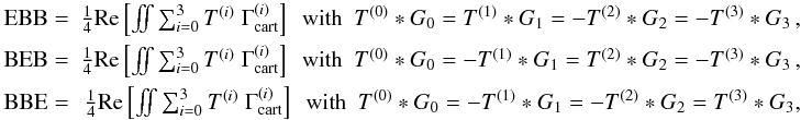 (67)and
 (68)For
all of them the condition that
T(0) ∗ G0 is real has been
imposed.
(68)For
all of them the condition that
T(0) ∗ G0 is real has been
imposed.
The four parity violating statistics (68) can be used as a check on parity violating systematical errors, while the other B-mode statistics (67) allows for a further examination of the B-modes.
With (52) one can easily invert the
conditions on the weight functions to express the weight function T’s
directly in terms of each other. Take the conditions for EEE (66) for example. One can write the Fourier transforms of
T(1), T(2) and
T(3) as functions of the Fourier transform of
T(0) as  (69)In order to
simplify these relations, we now attempt to give simple expressions for
(69)In order to
simplify these relations, we now attempt to give simple expressions for
 for i = 1,2,3. With (51)
one has
for i = 1,2,3. With (51)
one has  ,
which does not depend on
ℓ2. Noticing that
,
which does not depend on
ℓ2. Noticing that
 (see Sect. 3.3), we actually have
 , which yields in
configuration space
, which yields in
configuration space 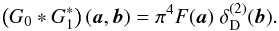 (70)Similarly one can derive
that
(70)Similarly one can derive
that  (71)Inserting (70) and (71) into (69), one
obtains
(71)Inserting (70) and (71) into (69), one
obtains  (72)
(72) (73)
(73) (74)where we have used the
expression of F (19).
(74)where we have used the
expression of F (19).
To summarize, if one chooses an arbitrary form of T(0) which
makes T(0) ∗ G0 real, constructs
T(1), T(2) and
T(3) according to (72), (73) and (74), and uses these weight functions to weight
the measured ’s,
then the resulting statistic EEE as defined in (64) receives contributions only from
⟨ κEκEκE ⟩
but not the terms affected by the B-mode. The B-mode statistics can be obtained from the
measured ’s
through a similar procedure. Equations (72)–(74) are the analogue
of (59) for 3-pt functions.
We note again that  ,
,
 and
and  are not independent under transformation of their arguments. Thus the statistics EEE (64) as well as the B-mode statistics (67) and (68) can all be written in terms of linear combinations of
and
alone. However we shall keep the current redundancy since it allows for simple analytical
expressions of the relations between the weight functions.
are not independent under transformation of their arguments. Thus the statistics EEE (64) as well as the B-mode statistics (67) and (68) can all be written in terms of linear combinations of
and
alone. However we shall keep the current redundancy since it allows for simple analytical
expressions of the relations between the weight functions.
So far one still has much freedom in choosing the form of T(0)(x1,x2). This freedom can be exploited to construct statistics which do not respond to the γ3PCF at smaller or larger angular separations than can be probed by the survey. We leave this to future work.
7. Numerical evaluation
7.1. Design of the sampling grid
We have written configuration space relations between weak lensing statistics in the form of convolutions, e.g. (23) and (24), where the convolution kernels are complex, have non-trivial spin numbers, and feature singularities. The convolutions can be performed numerically, but special care must be taken of these properties of the integration kernel.
One can take the K-S kernel −1/z ∗ 2 as an example of this kind of convolution kernel. The K-S kernel has an integer spin of 2, so an azimuthal integration of the kernel around its singularity at z = 0 should give zero, i.e. the values of the kernel along the circle cancel themselves due to their opposite phases. This property renders its singularity harmless, but entails the condition that the sampling grid should guarantee the cancellation. Such a requirement of a special grid design has already been realized in early lensing mass reconstruction works (e.g. Seitz & Schneider 1996). For a spin-2 kernel like the K-S kernel, a common square grid already suffices if the singularity is placed at a center of rotational symmetry, i.e. either onto a grid point or at the center of four grid points. In the case of the former, the grid point at the singularity has to be discarded. The latter, as shown by the left panel in Fig. 2, is a better choice considering the sampling homogeneity.
 |
Fig. 2 Examples of sampling grids applicable for 2D integration over singular kernels of different spin values. The cross in the center indicates the position of the singularity in the integration kernel. |
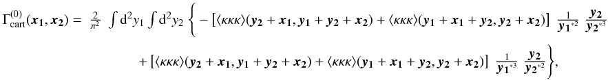
In general we need to deal with convolution kernels with different spin numbers. For example, the kernel F between γ2PCF and κ2PCF (19), which is proportional to z/z ∗ 3, has a spin of 4. In this case the square grid cannot guarantee the phase cancellation around the singularity any more (see Fig. 3). With a similar analysis as shown in Fig. 3, one can see that a triangular grid (middle panel, Fig. 2) can actually guarantee the phase cancellation around the singularity of a spin-4 kernel. When using a triangular grid, the singularity can also be put either on a grid point or at the center of three grid points. The former choice loses the grid point at the singularity, but is applicable to spin-3 kernels where the latter fails.
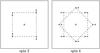 |
Fig. 3 A square grid guarantees phase cancellation around the singularity of spin-2 kernels (left panel), but not that of spin-4 kernels (right panel). The crosses indicate the position of the singularity of the integration kernel, while the dots are the grid points closest to the singularity. The polar angles of the kernel at the grid points are indicated by the directions of the arrows. For a spin-2 kernel they cancel each other on a square grid already. For a spin-4 kernel they cancel each other if the square grid is duplicated, rotated 45 degrees and put on top of the original grid. |
To achieve a high numerical accuracy, it is required that the circle integral around the singularity is well-sampled. If one uses a square (triangular) grid, the innermost circle is only sampled by four (six) grid points, which is not enough for many κ-models. To remedy this, one can duplicate the sampling grid, rotate it around the singularity, and put it on top of the original grid. We show the result with the square grid and 45 degrees of rotation in the right panel of Fig. 2. The resulting grid is also applicable for spin-4 kernels, as shown in the right panel of Fig. 3. This non-standard way of constructing sampling grids, although not creating the best grids in terms of sampling efficiency, deals very well with the singularity of the integration kernel, and can easily generate sampling grids applicable for kernels of any spin number. We use this kind of grid in our numerical sampling.
Additional complications arise when performing the integration for 3-pt statistics. There
are two 2D integrals in (4), (36), (37) and (38). The corresponding
integration kernels (22), (45), (46) and (47) all have three
singularities. Luckily we can split each integration kernel into four additive terms and
perform the integrals over each of them separately. Moreover, one can apply translational
shifts to the integrands so that in each 2D integral there is only one singularity in the
integration kernel. The singularity can also be shifted to the origin of the grids for
numerical simplicity. After all these procedures, the four relations can be written as
 (75)
(75) (76)
(76) (77)
(77) (78)We
can see that the integration kernels are either spin-2, spin-4, or spin-3. All sampling
grids shown in Fig. 2 are applicable to spin-3
kernels.
(78)We
can see that the integration kernels are either spin-2, spin-4, or spin-3. All sampling
grids shown in Fig. 2 are applicable to spin-3
kernels.
7.2. Numerical results for 2PCF
We now construct several toy models for 2-pt and 3-pt convergence and shear correlations, and use them to test the relations derived as well as the numerical sampling method.
In the 2-pt case, we build two models for the convergence correlation function: ⟨κκ⟩(r) = 1/r, and ⟨κκ⟩(r) = e−r2. Using the well-established ξ+ − ξ− relation (1) we can obtain the corresponding models for the shear correlation function: ⟨γγ⟩(r) = e4iφr/r, and ⟨γγ⟩(r) = e4iφr [(r4 + 4r2 + 6) e−r2 + 2r2 − 6] /r4.
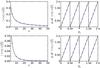 |
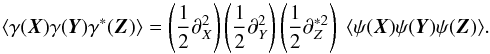
Fig. 4 Left panels: ⟨ γγ ⟩ (r) with fixed φr = π/6 as a function of r. Right panels: polar angle of ⟨ γγ ⟩ (r) with fixed r = 20 as a function of φr. The black curves are the expected values while the dots are the results from numerical evaluation of 2D integral in (23). The ⟨ κκ ⟩ used in the upper panels is ⟨ κκ ⟩ (r) = 1/r and in the lower panels ⟨ κκ ⟩ (r) = exp(−r2). |
Figure 4 shows the comparison between these shear correlation function models and the shear correlation functions sampled using (23), with the corresponding convergence correlation function models as input. The numerically sampled values match the analytical models very well.
7.3. Numerical results for 3PCF
We build models for 3pt shear and convergence correlation functions via the 3pt
correlation function of the deflection potential ψ. Suppose we evaluate
the fields at positions X, Y and Z. By
definition we have 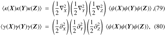 and
and
 (81)Now we assume a
model for
⟨ ψ(X)ψ(Y)ψ(Z) ⟩
as
(81)Now we assume a
model for
⟨ ψ(X)ψ(Y)ψ(Z) ⟩
as 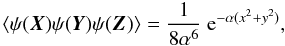 (82)with
x = X − Z
and
y = Y − Z.
This model is special in the sense that it does not depend on the angle between
x and y, but is
nevertheless simple and rather local. The statistical homogeneity of the field enables us
to write the 3pt correlation function as a function of two 2D spatial coordinates, which
we have chosen here to be x and
y.
(82)with
x = X − Z
and
y = Y − Z.
This model is special in the sense that it does not depend on the angle between
x and y, but is
nevertheless simple and rather local. The statistical homogeneity of the field enables us
to write the 3pt correlation function as a function of two 2D spatial coordinates, which
we have chosen here to be x and
y.
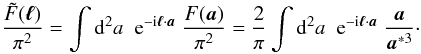
Performing the derivatives, we find the corresponding 3pt shear and convergence
correlation functions also depend only on
X − Z = x
and
Y − Z = y,
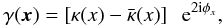
and read ![Mathematical equation: \begin{eqnarray} \label{eq:3pk} \langle \kappa\kappa\kappa\rangle (\vek{x}, \vek{y}) &=& \Big[-4 +\alpha\br{6(x^2+y^2)+8 \vek{x}\cdot\vek{y}} - \alpha^2 \Big((x^2+y^2)^2 +4(x^2+y^2) \vek{x}\cdot\vek{y} +6 x^2 y^2 \Big)+\alpha^3 x^2 y^2 |\vek{x}+\vek{y}|^2 \Big]\; \frac{\expo{-\alpha (x^2+y^2)}}{\alpha^3},\quad\quad\quad\quad\quad\quad\\ \label{eq:3pg0} \langle \gamma\gamma\gamma\rangle (\vek{x}, \vek{y}) &=& \vek{x}^2\vek{y}^2(\vek{x}+\vek{y})^2\expo{-\alpha (x^2+y^2)}, \end{eqnarray}](/articles/aa/full_html/2011/09/aa17236-11/aa17236-11-eq294.png) and
and
 (85)Using (83) as the input model for
⟨ κκκ ⟩ , we numerically evaluate
⟨ γγγ ⟩ (x,y)
and
⟨ γγγ∗ ⟩ (x,y)
using (75) and (78). The results are then compared to the
analytical models for the 3pt shear correlation functions (84) and (85). As shown
in Fig. 5, the numerical evaluations closely match
the analytical models.
(85)Using (83) as the input model for
⟨ κκκ ⟩ , we numerically evaluate
⟨ γγγ ⟩ (x,y)
and
⟨ γγγ∗ ⟩ (x,y)
using (75) and (78). The results are then compared to the
analytical models for the 3pt shear correlation functions (84) and (85). As shown
in Fig. 5, the numerical evaluations closely match
the analytical models.
Hence, we have proven numerically that the relations between γ3PCFs and κ3PCFs (75) and (78) are correct, no additional delta functions are needed. At the same time we have shown that these relations can be numerically evaluated with a high accuracy. Therefore these relations provide a better way of relating the observable shear signal to the underlying matter density field than the original way, i.e. using the relations between the γ3PCFs and the κ bispectrum, since the latter does not allow for an easy accurate numerical evaluation.
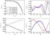 |
Fig. 5 Comparison of numerically evaluated ⟨ γγγ ⟩ (x,y) and ⟨ γγγ∗ ⟩ (x,y) with their analytical toy models described in this section adopting α = 0.05. “Re” and “Im” indicate the real and imaginary parts of the shear correlation functions. Left panels: the functions are evaluated at x = 0.25k e−iπ/3 and y = 0.17k eiπ/8 for different values of k; right panels: the functions are evaluated at x = 0.75 e−iπ/3 and y = 0.45 eiφ for 50 equally spaced φ values. |
8. Conclusion
We derived the relations between the 3-pt shear and convergence correlation functions which had been an important missing link between weak lensing three-point statistics. As an intermediate step, we found the 2-pt analogue of these relations and proved that it is the non-symmetrized form of the existing ξ+ − ξ− relation. By drawing analogy to the corresponding 1-pt relations, namely the Kaiser-Squires relation and its isotropic form, we have further revealed that the newly derived relations and already established results fit into the same theoretical framework. The consistency of the configuration space relations with the known Fourier space relations have also been shown.
The 3-pt relations derived are simple both analytically and numerically. They can be used as an alternative way of relating the measurable 3-pt weak lensing statistics with the statistics of the underlying matter density field. Up to now one has to use the relations between the γ3PCFs and the convergence bispectrum to link theory to the observable 3-pt shear signal. Since the γ3PCFs are very oscillatory and complicated functions of the convergence bispectrum (Schneider et al. 2005), it is hard to study the behavior of the 3-pt shear signal for a given convergence bispectrum model. With the relations we derived, one can instead study the properties of the 3-pt shear signal by constructing models for the κ3PCFs.
The method we used to derive these relations is based on the relation between the 2-pt correlation functions of the lensing deflection potential and the convergence. The same method also allows one to systematically derive the relations between correlations functions of other weak lensing quantities, including the deflection potential ψ, the shear γ, the convergence κ, and the deflection angle α. We present the forms of some 2- and 3-pt relations in Appendix B. Some of them are potentially of interest for studies of galaxy-galaxy(-galaxy) lensing and lensing of the cosmic microwave background.
Since the relations we obtained have complex kernels with non-trivial spin number and singularities, special care is needed when they are used numerically. We demonstrated how the numerical evaluation can be done, in particular the design of the sampling grid. Examples of numerical evaluation were shown for both 2- and 3-pt relations using toy models for the convergence correlation function. Their results match very well with the analytical expectations.
Separating E- and B-modes from measurements of the γ3PCFs is particularly important since the systematic effects at the 3-pt level are less understood. So far the only 3-pt statistics allowing for an E/B-mode decomposition is the aperture mass statistics (Jarvis et al. 2004; Schneider et al. 2005) which is plagued with the same problem as the 2-pt aperture statistics pointed out by Kilbinger et al. (2006). To amend this problem, one needs to construct the 3-pt correspondence of the newly developed 2-pt statistics (Schneider & Kilbinger 2007; Eifler et al. 2010; Fu & Kilbinger 2010; Schneider et al. 2010) which allows for an E/B-mode decomposition on a finite interval. As a direct theoretical application of the 3-pt relations derived in this paper, we used them to formulate the conditions for E/B-mode decomposition of lensing 3-pt statistics, in analogy to the 2-pt condition given by Schneider & Kilbinger (2007). These conditions are the basis of formulating additional constraints which lead to E/B-mode decomposition over a finite region, therefore they provide a starting point for future works on constructing better 3-pt shear statistics.
Our work was done for the case of weak lensing, but since it has only used the mathematical structure of the shear and the convergence, it applies also to other 2D polarization fields such as the polarization fluctuations of the cosmic microwave background.
Acknowledgments
X.S. would like to thank Fujun Du, Guangxing Li, and Andy Taylor for helpful discussions. B.J. acknowledges support by a UK Space Agency Euclid grant. This work was supported by the Deutsche Forschungsgemeinschaft under the Collaborative Research Center TR-33 “The Dark Universe” and the EC within the RTN Network “DUEL”.
References
- Bartelmann, M., & Schneider, P. 2001, Phys. Rep., 340, 291 [NASA ADS] [CrossRef] [Google Scholar]
- Bernardeau, F., Mellier, Y., & van Waerbeke, L. 2002, A&A, 389, L28 [Google Scholar]
- Bunn, E. F. 2011, Phys. Rev. D, 83, 083003 [NASA ADS] [CrossRef] [Google Scholar]
- Bunn, E. F., Zaldarriaga, M., Tegmark, M., & de Oliveira-Costa, A. 2003, Phys. Rev. D, 67, 023501 [NASA ADS] [CrossRef] [Google Scholar]
- Crittenden, R. G., Natarajan, P., Pen, U., & Theuns, T. 2002, ApJ, 568, 20 [NASA ADS] [CrossRef] [Google Scholar]
- Eifler, T., Schneider, P., & Krause, E. 2010, A&A, 510, A7 [NASA ADS] [CrossRef] [EDP Sciences] [Google Scholar]
- Erben, T., Hildebrandt, H., Lerchster, M., et al. 2009, A&A, 493, 1197 [NASA ADS] [CrossRef] [EDP Sciences] [Google Scholar]
- Fu, L., & Kilbinger, M. 2010, MNRAS, 401, 1264 [NASA ADS] [CrossRef] [Google Scholar]
- Gradshteyn, I. S., Ryzhik, I. M., Jeffrey, A., & Zwillinger, D. 2000, Table of Integrals, Series, and Products (Academic Press) [Google Scholar]
- Hu, W. 2000, Phys. Rev. D, 62, 043007 [NASA ADS] [CrossRef] [Google Scholar]
- Jarvis, M., Bernstein, G., & Jain, B. 2004, MNRAS, 352, 338 [NASA ADS] [CrossRef] [Google Scholar]
- Kaiser, N., & Squires, G. 1993, ApJ, 404, 441 [NASA ADS] [CrossRef] [Google Scholar]
- Kilbinger, M., & Schneider, P. 2005, A&A, 442, 69 [NASA ADS] [CrossRef] [EDP Sciences] [Google Scholar]
- Kilbinger, M., Schneider, P., & Eifler, T. 2006, A&A, 457, 15 [Google Scholar]
- Pen, U., Van Waerbeke, L., & Mellier, Y. 2002, ApJ, 567, 31 [NASA ADS] [CrossRef] [Google Scholar]
- Pen, U.-L., Zhang, T., van Waerbeke, L., et al. 2003, ApJ, 592, 664 [NASA ADS] [CrossRef] [Google Scholar]
- Schneider, P. 2003, A&A, 408, 829 [NASA ADS] [CrossRef] [EDP Sciences] [Google Scholar]
- Schneider, P. 2006, in Saas-Fee Advanced Course 33: Gravitational Lensing: Strong, Weak and Micro, ed. G. Meylan, P. Jetzer, P. North, et al., 269 [Google Scholar]
- Schneider, P., & Kilbinger, M. 2007, A&A, 462, 841 [NASA ADS] [CrossRef] [EDP Sciences] [Google Scholar]
- Schneider, P., & Lombardi, M. 2003, A&A, 397, 809 [NASA ADS] [CrossRef] [EDP Sciences] [Google Scholar]
- Schneider, P., Ehlers, J., & Falco, E. E. 1992, Gravitational Lenses (Springer-Verlag) [Google Scholar]
- Schneider, P., van Waerbeke, L., & Mellier, Y. 2002, A&A, 389, 729 [NASA ADS] [CrossRef] [EDP Sciences] [Google Scholar]
- Schneider, P., Kilbinger, M., & Lombardi, M. 2005, A&A, 431, 9 [NASA ADS] [CrossRef] [EDP Sciences] [Google Scholar]
- Schneider, P., Eifler, T., & Krause, E. 2010, A&A, 520, A116 [NASA ADS] [CrossRef] [EDP Sciences] [Google Scholar]
- Seitz, S., & Schneider, P. 1996, A&A, 305, 383 [NASA ADS] [Google Scholar]
- Semboloni, E., Schrabback, T., van Waerbeke, L., et al. 2011, MNRAS, 410, 143 [NASA ADS] [CrossRef] [Google Scholar]
Appendix A: Fourier transform of the F and G0 kernels
The F and G0 kernels, as defined in (7) and (4) relate the 2- and 3-pt shear and convergence correlation functions, respectively. In Sect.2 we have derived their explicit forms, see (19) and (22). According to the Fourier space relations of the shear and convergence statistics (31) and (32), one expects that F/π2 and e4iβ are Fourier pairs, as well as −G0/π3 and e2i(β1 + β2 + β3). Here we perform the Fourier transforms of F/π2 and −G0/π3, with F and G0 given in (19) and (22).
The Fourier transformation of the kernel F is a 2D integral of the form
 (A.1)The Fourier
transformation of the kernel G0 can be greatly simplified by
performing translational shifts to the integration variables. It turns out that the full
transformation is composed of 2D integrals similar to that in (A.1),
(A.1)The Fourier
transformation of the kernel G0 can be greatly simplified by
performing translational shifts to the integration variables. It turns out that the full
transformation is composed of 2D integrals similar to that in (A.1),
 (A.2)Performing
the 2D integrals in polar coordinates results in
(A.2)Performing
the 2D integrals in polar coordinates results in  (A.3)
(A.3)
 (A.4)
(A.4)
 (A.5)and
 (A.6)Combining (A.1) and (A.3) yields
 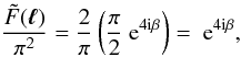 (A.7)which demonstrates that
the Fourier transformation of F/π2 is
indeed the phase factor e4iβ in (31).
(A.7)which demonstrates that
the Fourier transformation of F/π2 is
indeed the phase factor e4iβ in (31).
For the G0 kernel we still need to take account that
ℓ3 = ℓ3 eiβ3 ≡ −ℓ1 − ℓ2,
so that 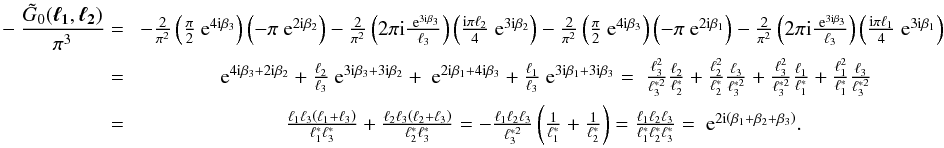 (A.8)Thus
the Fourier transformation of
−G0/π3 equals the phase
factor
e2i(β1 + β2 + β3)
in (32), as expected.
(A.8)Thus
the Fourier transformation of
−G0/π3 equals the phase
factor
e2i(β1 + β2 + β3)
in (32), as expected.
Appendix B: Relations between other correlation functions
In Sect. 2.2 we have derived the relations between
the shear and the convergence 2- and 3-pt correlation functions. The method we used is
based on the relation between the 2-pt correlation functions of the convergence
κ and the deflection potential ψ (12). Thus the method can easily be generated
to derive relations between the correlation function of κ and that of any
weak lensing quantity g which can be expressed as derivatives of
ψ. We denote g = Dgψ, and
write these 2-pt relations in a general form 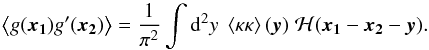 (B.1)
(B.1)
Listed below are some candidates for g and the corresponding operator Dg, where α is the deflection angle defined as α = ∂ψ.
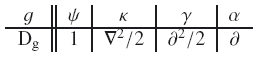
Let DgDg′ act on both sides of the relation between ⟨ψψ⟩ and ⟨κκ⟩ (11), and use the statistical homogeneity of the κ field, one can obtain an integration form of the kernel ℋ, in analogy to (8). Let the same operator act on both sides of (12), one can express ℋ as derivatives of the convolution kernel ℱ in (12), as ℋ(x1 − x2 − y) = DgDg′ℱ(x1 − x2 − y). Further inserting the explicit form of ℱ (19) allows one to obtain the explicit form of ℋ as a function of z = x1 − x2 − y. We summarize some of the 2-pt relations in Table B.1. Note that the form of ℋ(ℱ) for ⟨αα⟩ has a minus sign, which is due to the fact that ∂x1∂x2ℱ(x1 − x2 − y) = −∂2ℱ(z) with z = x1 − x2 − y.
We write the relations between ⟨κκκ⟩ and the 3-pt correlation functions
of the g’s also in a uniform convolutional form,  (B.2)To find the explicit
form of the convolution kernel I, we first write it into an integral
form, in analogy to (6), and then split it
into terms which can be expressed also as derivatives of the kernel ℱ, like (20). Then with the explicit form of ℱ one can
reach the explicit form of I. We list the forms of the convolution kernel
I for some 3-pt statistics in Table B.2.
(B.2)To find the explicit
form of the convolution kernel I, we first write it into an integral
form, in analogy to (6), and then split it
into terms which can be expressed also as derivatives of the kernel ℱ, like (20). Then with the explicit form of ℱ one can
reach the explicit form of I. We list the forms of the convolution kernel
I for some 3-pt statistics in Table B.2.
Some of these relations, e.g. those for ⟨κγ⟩, ⟨γγκ⟩, and ⟨γκκ⟩, can find their application in galaxy-galaxy(-galaxy) lensing. Some other relations, e.g. those for ⟨αα⟩, ⟨ακ⟩, and ⟨αακ⟩, are potentially of interest for studies of the lensing effects on the cosmic microwave background and its cross-correlation with galaxy weak-lensing maps (Hu 2000).
All Tables
All Figures
|
Fig. 1 Definition of the geometry of a triangle (the leftmost sketch) and how it changes under permutations (the first three sketches from the left) and flip (the leftmost and the rightmost sketch) of the vertices. |
| In the text | |
|
Fig. 2 Examples of sampling grids applicable for 2D integration over singular kernels of different spin values. The cross in the center indicates the position of the singularity in the integration kernel. |
| In the text | |
|
Fig. 3 A square grid guarantees phase cancellation around the singularity of spin-2 kernels (left panel), but not that of spin-4 kernels (right panel). The crosses indicate the position of the singularity of the integration kernel, while the dots are the grid points closest to the singularity. The polar angles of the kernel at the grid points are indicated by the directions of the arrows. For a spin-2 kernel they cancel each other on a square grid already. For a spin-4 kernel they cancel each other if the square grid is duplicated, rotated 45 degrees and put on top of the original grid. |
| In the text | |
|
Fig. 4 Left panels: ⟨ γγ ⟩ (r) with fixed φr = π/6 as a function of r. Right panels: polar angle of ⟨ γγ ⟩ (r) with fixed r = 20 as a function of φr. The black curves are the expected values while the dots are the results from numerical evaluation of 2D integral in (23). The ⟨ κκ ⟩ used in the upper panels is ⟨ κκ ⟩ (r) = 1/r and in the lower panels ⟨ κκ ⟩ (r) = exp(−r2). |
| In the text | |
|
Fig. 5 Comparison of numerically evaluated ⟨ γγγ ⟩ (x,y) and ⟨ γγγ∗ ⟩ (x,y) with their analytical toy models described in this section adopting α = 0.05. “Re” and “Im” indicate the real and imaginary parts of the shear correlation functions. Left panels: the functions are evaluated at x = 0.25k e−iπ/3 and y = 0.17k eiπ/8 for different values of k; right panels: the functions are evaluated at x = 0.75 e−iπ/3 and y = 0.45 eiφ for 50 equally spaced φ values. |
| In the text | |
Current usage metrics show cumulative count of Article Views (full-text article views including HTML views, PDF and ePub downloads, according to the available data) and Abstracts Views on Vision4Press platform.
Data correspond to usage on the plateform after 2015. The current usage metrics is available 48-96 hours after online publication and is updated daily on week days.
Initial download of the metrics may take a while.