| Issue |
A&A
Volume 533, September 2011
|
|
|---|---|---|
| Article Number | A19 | |
| Number of page(s) | 12 | |
| Section | Extragalactic astronomy | |
| DOI | https://doi.org/10.1051/0004-6361/201117004 | |
| Published online | 18 August 2011 | |
Studying the spatially resolved Schmidt-Kennicutt law in interacting galaxies: the case of Arp 158
1
University of MassachusettsDepartment of Astronomy,,
LGRT-B 619E,
Amherst,
MA
01003,
USA
2
Laboratoire d’Astrophysique de Marseille, UMR 6110
CNRS, 38 rue F.
Joliot-Curie, 13388
Marseille,
France
e-mail: This email address is being protected from spambots. You need JavaScript enabled to view it.
3 Departamento de Física Teórica y del Cosmos, Universidad de
Granada, Spain
4
Laboratoire AIM, CEA/DSM – CNRS – Université Paris Diderot,
DAPNIA/Service d’Astrophysique, CEA/Saclay, 91191
Gif-sur-Yvette Cedex,
France
5
Laboratoire d’Astrophysique de Bordeaux, Université Bordeaux 1,
Observatoire de Bordeaux, OASU, UMR 5804, CNRS/INSU, BP 89, 33270
Floirac,
France
6
Centre for Astrophysics Research, University of
Hertfordshire, Hatfield
AL10 9AB,
UK
7
Department of Physics and Institute of Theoretical &
Computational Physics, University of Crete, 71003
Heraklion,
Greece
8
IESL/Foundation for Research and Technology –
Hellas, 71110
Heraklion,
Greece
9
Chercheur Associé, Observatoire de Paris,
75014
Paris,
France
Received: 1 April 2011
Accepted: 30 June 2011
Abstract
Context. Recent studies have shown that star formation in mergers does not seem to follow the same Schmidt-Kennicutt relation as in spiral disks, presenting a higher star formation rate (SFR) for a given gas column density.
Aims. In this paper we study why and how different models of star formation arise. To do so we examine the process of star formation in the interacting system Arp 158 and its tidal debris.
Methods. We perform an analysis of the properties of specific regions of interest in Arp 158 using observations tracing the atomic and the molecular gas, star formation, the stellar populations as well as optical spectroscopy to determine their exact nature and their metallicity. We also fit their spectral energy distribution with an evolutionary synthesis code. Finally, we compare star formation in these objects to star formation in the disks of spiral galaxies and mergers.
Results. Abundant molecular gas is found throughout the system and the tidal tails appear to have many young stars compared to their old stellar content. One of the nuclei is dominated by a starburst whereas the other is an active nucleus. We estimate the SFR throughout the systems using various tracers and find that most regions follow closely the Schmidt-Kennicutt relation seen in spiral galaxies with the exception of the nuclear starburst and the tip of one of the tails. We examine whether this diversity is due to uncertainties in the manner the SFR is determined or whether the conditions in the nuclear starburst region are such that it does not follow the same Schmidt-Kennicutt law as other regions.
Conclusions. Observations of the interacting system Arp 158 provide the first evidence in a resolved fashion that different star-forming regions in a merger may be following different Schmidt-Kennicutt laws. This suggests that the physics of the interstellar medium at a scale no larger than 1 kpc, the size of the largest gravitational instabilities and the injection scale of turbulence, determines the origin of these laws.
Key words: galaxies: star formation / galaxies: interactions
© ESO, 2011
1. Introduction
How atomic gas turns molecular and forms stars is one of the questions that is paramount to understanding the process of star formation in galaxies. This process plays a fundamental role in the transformation of baryonic matter and is the main driver of galaxy formation and evolution. It is well known that star-formation depends on the local physical conditions of the gas such as the pressure. It depends on the molecular gas column density by way of the Schmidt-Kennicutt law (Schmidt 1959; Kennicutt 1998b; Kennicutt et al. 2007; Leroy et al. 2008; Bigiel et al. 2008). On the large scale it is, however, still not well understood how star formation depends on feedback, spiral density waves or shear, and more generally on the global environment such as in the case of mergers (Barnes 2004; Chien & Barnes 2010; Teyssier et al. 2010; Bournaud et al. 2011).
Regions of interest.
One way to test for the effect of the environment is to use star-forming regions located in collisional debris which are the offsprings of galaxy interactions. Indeed, depending on the parameters of the collision (relative velocity, impact factor, prograde versus retrograde, etc.), a varying amount of gas and stars can be stripped from the parent galaxies and injected into the intergalactic medium. In addition to atomic gas pulled from the parent galaxies, these collisional debris actually contain surprisingly large amounts of molecular gas formed in-situ (Braine et al. 2000, 2001; Lisenfeld et al. 2002, 2004; Petitpas & Taylor 2005; Duc et al. 2007). As the gas subsequently collapses, star-forming regions are created with masses ranging from a few hundred solar masses, creating OB associations, the “emission line dots” (Gerhard et al. 2002; Yoshida et al. 2002; Sakai et al. 2002; Weilbacher et al. 2003; Ryan-Weber et al. 2004; Mendes de Oliveira et al. 2004; Cortese et al. 2006; Werk et al. 2008, 2010) to objects as massive as dwarf galaxies named tidal dwarf galaxies (TDGs, Duc 1995; Duc & Mirabel 1998; Duc et al. 2000, 2007; Hancock et al. 2007, 2009). These objects, even though formed from material once pertaining to their parent galaxies, have a radically different and simpler environment. Recently, Boquien et al. (2007, 2009) showed that star-formation tracers such as ultraviolet, mid-infrared, and Hα, are as reliable in intergalactic star-forming regions as they are in spiral galaxies. Braine et al. (2001) showed that the depletion timescale of the molecular gas is similar to that of spiral galaxies even though the collision debris they studied have the luminosity, mass and colour of dwarf galaxies. As collision debris probably have a conversion factor close to that of spiral galaxies with a solar neighbourhood metallicity, this eliminates a major source of uncertainty.
There are still many open questions regarding star-formation in collision debris and how the process compares to star formation in spiral disks or in other environments. It has been observed that star formation is particularly efficient in ultraluminous infrared galaxies (ULIRGs) deduced from a high L(TIR)/L(CO) (Solomon & Vanden Bout 2005), as well as in galaxies that have a subsolar metallicity (Leroy et al. 2006; Gardan et al. 2007; Gratier et al. 2010; Braine et al. 2010). Conversely, other systems like intergalactic collisional gas bridges contain molecular gas but form stars inefficiently, such as the UGC 813/6 pair (Braine et al. 2004). Recent results by Daddi et al. (2010) and Genzel et al. (2010) showed that starbursts and mergers follow different modes of star formation compared to more quiescent spiral galaxies. Starbursts appear to be forming stars at a higher rate than spiral galaxies for the same gas column density. However, the discrepancy between the 2 regimes is increased by the use of a different XCO conversion factor between star-forming galaxies and starbursting ones. Can we observe such a difference within a single interacting system, hence retrieving this result in a resolved fashion? Are there deviations in the Schmidt-Kennicutt law between intergalactic star formation regions and what is seen in galactic disks (Bigiel et al. 2008)?
To address these questions we compare star formation in different parts of a single interacting system, Arp 158, and its tidal debris. This system is particularly suited for this study as it presents evidence of extended star formation. Using an homogeneous dataset on a single system means there are no internal calibration or methodological differences for the study of star formation in the interacting galaxies and their tidal debris. Arp 158 is an intermediate-stage merger in the Toomre (1977) sequence, with the disks progressively merging but still with 2 clearly separated nuclei. With a recession velocity cz = 4758 km s-1, Arp 158 is located at a luminosity distance of 62.1 Mpc1, assuming H0 = 73 km s-1 Mpc -1, Ωm = 0.27 and ΩΛ = 0.73, which corresponds to a scale of 292 pc/arcsec. To carry out this work we use multi-wavelength data, ranging from the far-ultraviolet to the radio, to trace star formation, the stellar populations and the atomic gas, also encompassing observations of the molecular component. Optically, the closely interacting galaxies have a boxy shape. They present a bar with 3 nearly aligned bright clumps. The nature of one of them, galactic nuclei or a foreground star, is debated in the literature (Chincarini & Heckathorn 1973; Dahari 1985). Prominent dust lanes are visible north of the bar. Two tidal tails can be seen, containing blue concentrations at their tips. The longer one, oriented towards the east-south-east, is a prime TDG candidate. The disks of the galaxies seem to be rather edge-on but their morphology is strongly disturbed making a precise assessment difficult. Radio 21 cm observations have shown that the entire system contains 6.5 × 10⁹ M⊙ of HI, with column density peaks at the tip of one of the tidal arms and towards the western nucleus (Iyer et al. 2004), providing a large reservoir of gas to fuel star formation throughout the system which yields an infrared luminosity of 3.1 × 10¹⁰ L⊙ (Sect. 3.3).
In Sect. 2 we present the multi-wavelength observations, followed by the results in Sect. 3 which we discuss in Sect. 4 before concluding in Sect. 5.
2. Observations and data reduction
In this section we present the set of multi-wavelength data we are using to carry out this study. For an easier description of the observations we have labelled different regions of interest in the system. These regions have been selected from the inspection of multi-wavelength data and concern the most interesting morphological features. The main characteristics of each object are briefly described in Table 1 and they are labelled on images of the system in Fig. 1.
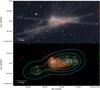 |
Fig. 1 Top: optical image in g′ (blue channel), r′ (green channel) and i′ (red channel) bands. The regions of interest listed in Table 1 are indicated with a red label. The white dashed rectangles represent the two long slits used for optical spectroscopy. Bottom: FUV (blue channel), NUV (green channel) and 24 μm (red channel). The contours in cyan trace the HI column density. The yellow dashed circles represent the CO(1–0) beams and the area in which fluxes have been measured. Due to the large CO beams, not all regions of interest can have their CO emission detected separately. |
Characteristics of the CO lines for the 5 pointings.
UV, optical and IR fluxes in the 5 CO pointing beams.
2.1. CO
To trace the molecular gas content of the system we have carried out CO observations with the 30 m millimetre-wave telescope on Pico Veleta (Spain) run by the Institut de Radio-Astronomie Millimétrique (IRAM). In November 2006 we observed positions C5 and NC with the A and B receivers. The observations of the positions NC, NE, C2 and C3 were done in January 2010 with the EMIR receiver. The CO(1–0) and CO(2–1) transitions at 115 GHz and 230 GHz, respectively, were observed simultaneously and in both polarisations. The redshifted frequencies were 113.4547 and 226.905 GHz, corresponding to a central velocity of cz = 4800 km s-1. For the November 2006 observations, we used the 512 × 1 MHz filterbanks at 3 mm, one for each polarisation, and the two 256 × 4 MHz filterbanks for the two polarisations at 1 mm, yielding instantaneous bandwidths of 1300 km s-1 in all transitions. The observations in January 2010 used the autocorrelator Wilma with a resolution of 2 MHz and for both the 90 GHz and 230 GHz band. The bandwidth was over 10 000 km s-1 for the CO(1–0) line and over 5000 km s-1 for the CO(2–1) line. All the observations were carried out in good weather conditions, the mean system temperatures being for the CO(1–0) transition 190 K (November 2006), and 245 K (January 2010), and for the CO(2–1) transition 330 K (November 2006), and 240 K (January 2010) on the  scale. The main beam efficiencies at Pico Veleta were taken to be at 115 GHz (0.74 and 0.77 for the A+B receivers and EMIR respectively), and at 230 GHz (0.54 and 0.58 for the A+B receivers and EMIR respectively). The halfpower beamwidths are about ~22 and ~11 arcsec, corresponding to physical sizes 6.4 kpc and 3.2 kpc. All observations were done in wobbler-switching mode, with a throw in azimuth between 150 and 220 arcsec. Pointing was checked on a nearby quasar roughly every 90 min.
Data reduction was straightforward: the spectra for each position were averaged. In most cases only zero-order baselines (i.e. continuum levels) were subtracted to obtain the final spectra, just in a few spectra a linear baseline had to be subtracted. Position NC was observed during both observing runs and allowed us to check the relative calibration. We found that the velocity integrated intensities were within 10% for CO(1–0) and CO(2–1). This constitutes the main source of uncertainty for the 3 brightest regions in CO. The characteristics of the lines are listed in Table 2.
2.2. HI
The HI data cube was obtained from the literature (Iyer et al. 2004). Observations of the atomic hydrogen were performed at the VLA (Very Large Array) in D configuration between 1999-05-14 and 1999-05-17 for a total of 5 h. The velocity resolution is 12.3 km s-1 and the final map resolution is 43.3″ × 42.2″ corresponding to a physical size of 12.3 kpc × 12.6 kpc. Data reduction is described in detail in Iyer et al. (2004).
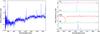 |
Fig. 2 Left: blue part of the spectrum of the NE clump. Several lines are clearly detected: [OII] 372.7, Hγ, [OIII] 436.3, Hβ, [OIII] 495.9, and [OIII] 500.7. Unfortunately the blue spectrum for other clumps is not deep enough to detect these emission lines. Right: spectra of clumps NE, NC, NW, C2, and C5. The spectra have been offset to distinguish them more easily. The spectra of clumps NC, NW, C2, and C5 are multiplied by 5 as they are intrinsically much fainter than the spectrum of NE. Except for NW, several lines are clearly detected: [NII] 654.8, Hα, [NII] 658.4, [SII] 671.7, and [SII] 673.1. The spectrum of NW shows a broad Hα line in absorption at almost 0-velocity with a weak Hα emission line at the recession velocity of Arp 158. |
2.3. Ultraviolet, optical and infrared imaging
Ultraviolet data have been obtained from the public archives of the GALEX space observatory. Observations were carried out on 2005–11–17 in the FUV (far ultraviolet; λeff = 151 nm) and NUV (near ultraviolet; λeff = 227 nm) bands in the context of the Guest Investigator programme GI2-019 (PI: Koratkar). Arp 158 is located ~3′ from the edge of the 1.24° field-of-view which is centered on NGC 507. The exposure time in FUV (NUV) is 3230 s (3398 s) leading to a sensitivity of 38 nJy px-1 (resp. 26 nJy px-1). The point spread function has a FWHM (full width half maximum) size of ~5″ corresponding to a physical size 1.5 kpc.
Shallow optical images have been obtained from SDSS (Sloan Digital Sky Survey) release 7 (Abazajian et al. 2009), tile 4829 in u′, g′, r′, i′ and z′ bands. Observations were carried out on 2004–09–15. Standard SDSS calibrations have been applied.
Shallow near-infrared images of the system were obtained from the 2MASS (2 Micron All Sky Survey, Skrutskie et al. 2006) archives. They are used exclusively for visual inspection.
Finally, Arp. 158 was observed by our team in the 24 μm band on 2009–02–07 using the Spitzer Space Observatory, programme ID 50191. The final exposure time per pixel is 10 s. The frames were processed by the standard Spitzer pipeline version 18.5.0. The processed image presents a smooth gradient in the background which was eliminated subtracting on each row the median of the sky.
Images of the system combining various wavelengths are presented in Fig. 1 along with the regions of interest identified.
Fluxes were measured in all images within circular apertures matching the CO(1–0) beam (about 22″ for the half-power beamwidth, Sect. 2.1 and Fig. 1) using the phot procedure from iraf. The background was taken as the mean of the median pixel value in several positions around the interacting system. The same background was subtracted for all apertures. Recent studies of nearby galaxies have shown the importance of background subtraction to derive the star-formation laws (Blanc et al. 2009; Rahman et al. 2011; Liu et al. 2011). However, this is most important for regions in galaxies forming stars at a low rate that can be resolved only in nearby galaxies. The distance of Arp 158, 62.1 Mpc, and the size of the regions selected limits the bias introduced by the background subtraction. The uncertainty on the background level is taken as the quadratic mean of the standard deviation of the background level measurements and the mean of the standard deviation of pixels within apertures in which the background is measured. Foreground extinction from the Milky Way was corrected in the UV and in the optical using the Cardelli et al. (1989) extinction law assuming E(B − V) = 0.054 from NED. The foreground extinction-corrected fluxes from FUV to 24 μm are presented in Table 3.
2.4. Optical spectroscopy
To gain insight into the physical nature of the selected regions and estimate their metallicity, we have also performed optical spectroscopy. Observations were carried out in service mode under good weather conditions at the William Herschel Telescope. Two long-slit spectra were obtained by our team using the ISIS (Intermediate dispersion Spectrograph and Imaging System) instrument with an exposure time of 1200 s. Each slit is 4′ long and 2″ wide. The first slit was aligned along the 3 bright condensations NE, NC, and NW, and the bar, with a position angle of 175.5°. The second one is aligned along the eastern tidal arm and the FUV bright condensation capturing clumps C1, C2 and C5, with a position angle of 15.5°. Each slit was observed using the R600R grating (dispersion of 0.50 Å/pixel) from 612 nm to 820 nm in the red arm of ISIS and the R600B grating (dispersion of 0.44 Å/pixel) from 360 nm to 540 nm in the blue arm of the instrument. An image of the system in the optical along with the position of the slits is presented in Fig. 1. Data reduction was carried out with the longslit package of iraf in a standard way. Flux calibration was carried out using the spectrophotometric star Feige 15 observed the same night. The emission lines were measured with splot within the iraf package. We present the data in Fig. 2.
In Table 4 we list the fluxes of the main emission lines we detected in the blue or red spectra depending on their wavelength.
Spectroscopic observations.
3. Results
3.1. Optical and near-infrared morphology
The optical image of the system is presented in the top panel in Fig. 1. Several features can be noted. First of all, as we mentioned earlier, there are 3 almost aligned bright concentrations, NE, NC and NW. At least 2 of them are galactic nuclei. The nature of the westernmost one, NW is uncertain. We will examine it further in Sect. 3.2. North of this alignment, we can see that there is a prominent dust lane. In the same alignment, we can see a tidal tail extending to the west. The smooth change of the brightness of the tail starting from the interacting galaxies suggests that it contains significant quantities of stars stripped from the parent galaxies which is confirmed by the fact that the tail is clearly seen in the near-infrared in 2MASS images. Another, more prominent, tidal tail is visible that extends from C4 to the east-south-east. This tail seems to be in the process of being detached from the parent galaxies as the drop in the brightness towards the centre of the tail suggests. In addition, it appears to be much fainter in the near-infrared compared to the northern one, probably because of the presence of fewer evolved stars in this tail. Conversely, its tip is much brighter and contains a number of blue knots suggesting on-going star formation.
SFR and extinction.
3.2. Metallicity of the clumps
Spectroscopic observations of the clumps allow us to ascertain their nature and determine the oxygen abundance for regions photo-ionised by massive stars. All 3 nuclei NE, NC, and NW exhibit some Hα emission, however the equivalent width is much larger in the case of NE. Examining the line ratios for each nucleus in the BPT diagram (Baldwin et al. 1981), it shows that NE is most likely a nuclear starburst. As for NC it suggests that it is an AGN, either an extreme LINER or a Seyfert. Finally, even though the Hα line is detected at the redshift of the system for NW the spectrum is typical of a star at zero velocity with a strong Balmer line in absorption, confirming the suggestion of Chincarini & Heckathorn (1973) that this compact object is a star in the Milky Way rather than a galactic nucleus. Upon close examination this is consistent with the morphology in the near-infrared images, with NW that seems more compact than NE or NC.
We calculate the oxygen abundance from strong emission lines. As the emission lines were not detected in the blue part of the spectrum except in the case of the NE clump (Fig. 2) we rely on the NII@658.4 nm to Hα ratio (Denicoló et al. 2002) which is little affected by the extinction due to the wavelength proximity of the two lines. This estimator is of course only valid for regions photo-ionised by massive stars and cannot be used in the case of AGN, which excludes region NC.
The oxygen abundances we estimate for photo-ionised regions are close to the solar one. In terms of 12 + log O/H, the eastern nucleus NE has 8.77 ± 0.07, C2 has 8.61 ± 0.09 and C5 has 8.72 ± 0.07. The 1-σ error bars are driven by the uncertainty on the N2 relation. Such a high metallicity for the tidal features is typical of this type of objects as gas is stripped from the radially mixed (Kewley et al. 2010) metal-rich parent galaxies.
3.3. Star formation rates and extinction
We determine the SFR both from the FUV emission and from the dust luminosity at 24 μm. The former one is sensitive to the photospheric emission of massive stars over a timescale of 100 × 106 years but is affected by internal extinction. The latter one is due to dust heated by massive stars but only probes star formation that is affected by extinction and can be contaminated by dust heating due to older stellar populations.
As we can see in Fig. 1, the morphology of the system as seen in star formation tracers is remarkably different from what can be seen in the optical bands. First of all, NE exhibits a particularly strong emission at 24 μm, which is consistent with the presence of a nuclear starburst. Emission at 24 μm can be seen throughout the rest of the interacting galaxies without any clear peak. Conversely, there is an UV peak for clump C3 with no corresponding peak at 24 μm. The tip of the westernmost tail, C2, also shows a strong peak at 24 μm with a weaker UV counterpart. In contrast C5 shows a strong UV peak with a weaker counterpart at 24 μm.
To estimate the SFR from the respective luminosities in those bands, we use: SFR(FUV) = 9.5 × 10⁻²² Lν(FUV), with Lν the luminosity density in W Hz-1 (Kennicutt 1998a), and ![Mathematical equation: \hbox{${{\it SFR}(24)=1.83\times\left[L(24)/10^{36}\right]^{0.83}}$}](/articles/aa/full_html/2011/09/aa17004-11/aa17004-11-eq167.png) , where L(24) is in W and is defined as νLν at 24 μm (Relaño et al. 2007) which is adapted for individual star-forming regions and provides results typically within 0.2 dex of other similar estimators (Calzetti et al. 2010). These estimators have been converted to a Kroupa (2001) IMF and assume a constant star formation rate over 100 Myr following Calzetti et al. (2007). As those bands are biased respectively against and towards extinction, we also estimate the SFR from the combination of these bands using Leroy et al. (2008) relation: SFR(24 + FUV) = 6.8 × 10⁻²²Lν(FUV) + 2.67 × 10⁻²³ Lν(24), with Lν in W Hz-1.
, where L(24) is in W and is defined as νLν at 24 μm (Relaño et al. 2007) which is adapted for individual star-forming regions and provides results typically within 0.2 dex of other similar estimators (Calzetti et al. 2010). These estimators have been converted to a Kroupa (2001) IMF and assume a constant star formation rate over 100 Myr following Calzetti et al. (2007). As those bands are biased respectively against and towards extinction, we also estimate the SFR from the combination of these bands using Leroy et al. (2008) relation: SFR(24 + FUV) = 6.8 × 10⁻²²Lν(FUV) + 2.67 × 10⁻²³ Lν(24), with Lν in W Hz-1.
Our spectroscopic observations do not allow us to correct for the extinction except in region NE. We have therefore decided to use the relation provided by Buat et al. (2005) to estimate the extinction in FUV from the ratio between the total infrared (TIR) emission and the FUV emission. Even though their relation was determined using galaxies rather than subregions in galaxies, the influence of the diffuse emission should remain minimal. Indeed the Buat et al. (2005) sample is mostly consistuted of late-type galaxies for which the diffuse emission is small (Sauvage & Thuan 1992). As we have only one infrared band, we use the following relation to estimate the TIR luminosity from the 24 μm luminosity provided for galaxy subregions by Boquien et al. (2010a): L(TIR) = 9.14 × 10⁴ L(24)0.887 with L(24) and L(TIR) in W. The extinction Av is determined from AFUV assuming a Calzetti (2001) attenuation curve. The SFR and estimates of the attenuation are presented in Table 5. These results are uncertain for the NC region due to the contamination by an active nucleus.
The uncorrected FUV yields a much lower SFR than 24 μm. This indicates that all regions suffer from strong extinction. This is particularly the case in strongly star-forming regions such as NE which has AV = 1.4 mag. The Balmer decrement for this region gives an extinction of approximatively AV = 2.1 mag. This is expected as the Balmer decrement measures the extinction of the gas. The relation of Buat et al. (2005) measures the extinction of the continuum, which is smaller (Calzetti 1997). More quiescent regions in the system have a smaller extinction, down to AV = 0.6 mag for C5. The combination of the FUV and 24 μm luminosities yields SFR that are higher than the FUV corrected ones for the 2 most extinguished regions and smaller than the FUV corrected ones for the others but no more than a factor of 1.5. IRAS (Infrared Astronomical Satellite) observations at 60 μm and 100 μm are a better estimator of the TIR as they trace the dust in thermal equilibrium with the radiation field at the peak of the emission. The total flux of the system is 0.24 Jy at 25 μm, assuming Fν(24) = Fν(25), 2.03 Jy at 60 μm and 4.51 Jy at 100 μm. Estimating the TIR using Eq. (5) from Dale & Helou (2002) we find 3.1 × 10¹⁰ L⊙ which yields SFR(IRAS) = 3.74 M⊙ yr-1 using equation 4 from Kennicutt (1998a) converted to a Kroupa (2001) IMF. The total SFR that we derived from 24+FUV is 2.89 M⊙ yr-1. This is only slightly lower than the IRAS value, most likely due to missing extended emission.
3.4. Gas properties
3.4.1. CO lines
CO(1–0) and CO(2–1) emission was detected for all pointings except for C2 for which there is a marginal detection in CO(1–0) and no detection in CO(2–1). The quality for the other positions is sufficient to determine the CO(2–1)/CO(1–0) ratios. The line ratios in NC (0.9 ± 0.1) and C3 (0.9 ± 0.1) are consistent with the average value found in nearby galaxies (0.89, Braine & Combes 1992), if the CO emission comes from a region roughly as large as the CO(1–0) beam. At these positions, optically thin emission, for which a line ratio >1 would be expected, can be excluded. Indeed, at the local thermodynamical equilibrium for a high temperature and high opacity we have CO(2–1)/CO(1–0) = 1. In the case of optically thin emission we expect line ratios >1 with an asymptotic case of CO(2–1)/CO(1–0) =  for optically thin gas in local thermodynamical equilibrium with a sufficiently high temperature (Wilson et al. 2009). Both the NE clump and C5 exhibit line ratios above 1 (1.3 ± 0.2 for the NE clump, and 1.5 ± 0.6 for C5). This could be due to (i) optically thin emission or (ii) emission concentrated to a region smaller than the CO(1–0) beam. Since both the 24 μm and the CO emission are strong at these positions, we think that option (ii) is more likely. Note however that the beam sizes are different which makes strong conclusions difficult.
3.4.2. Gas masses
We calculate the molecular masses using Eq. (1) from Braine et al. (2001): 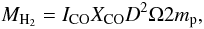 (1)where ICO is the observed line intensity in the beam in units of K km s-1, XCO is the conversion factor to estimate the molecular mass from CO taken as 2 × 1020 cm-2 (K km s-1)-1, D the distance of the system, Ω the solid angle of the beam (1.13θ2, θ being the beam FWHM), and mp the mass of a proton. Similarly to Bigiel et al. (2008), we do not take into account the helium mass to compute the molecular mass. It corresponds to MH2 = 75 ICOD2Ω, with MH2 in M⊙, ICO in K km s-1, D in Mpc, and Ω in arcsec2.
The low resolution of HI data makes it difficult to determine the HI mass within the CO(1–0) beam, especially in the main bodies of the galaxies. As C5 is relatively well isolated from the rest of the interacting system it is easier to measure its HI mass. However, rather than examining the mass encompassed in the CO(1–0) beam, we look at the column density in the pixel corresponding to the centre of the CO(1–0) beam in order to limit the blending with the HI emission from nearby regions. The derived molecular gas mass as well as molecular and atomic gas column densities are presented in Table 6.
Atomic, molecular gas mass and column density in the 5 CO pointing beams.
The system contains large amounts of molecular gas, particularly in the nuclei. However, the CO-to-H2 conversion factor is uncertain in these environments and it is likely that there is more CO emission per unit H2 in galactic centres. The molecular mass in the tidal features is lower, 5.8 × 10⁷ M⊙ in C2 and 6.8 × 10⁷ M⊙ in C5. Comparing to the sample of TDG candidates of Braine et al. (2001), it is in the lower range of observed molecular masses.
Both nuclei are significantly dominated by their molecular phase, which is commonly observed in the centre of spiral galaxies (Bigiel et al. 2008). C5, on the other hand, is HI dominated and its molecular to atomic gas mass ratio is typical of what is observed in collision debris (Braine et al. 2001).
3.5. Kinematics of the system
A comparison of the HI, CO(1–0) and CO(2–1) spectra of the four CO-detected regions is presented in Fig. 3.
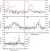 |
Fig. 3 Spectra of the five regions. CO(1–0) is shown in black, CO(2–1) in green, and HI in red. The HI spectra correspond to the central pixel in the CO beam in order to limit the blending with adjacent sources. We have multiplied the flux of the CO spectra by 5 in the case of C2 and C5 to make them more visible. All spectra have been centred to a velocity of 4800 km s-1. |
The recession velocity of the system that we determined through optical spectroscopy, CO and HI observations is consistent with the value of 4758 km s-1 mentioned in the introduction. The system rotates clockwise, the C5 and NE regions having a recession velocity comprised between 4900 km s-1 and 5000 km s-1 whereas the western C3 and C2 regions have a smaller velocity between 4500 km s-1 and 4700 km s-1.
The NE region presents a double-peaked profile centered around 4950 km s-1. It is most prominent in CO(2–1) in which the peaks are separated by a velocity of 70 km s-1. The peaks are not as strong in CO(1–0) and HI, probably due to additional contamination because of the larger beam. This may be the signature of a rotating ring of star formation in the nucleus of the galaxy with blueshifted and redshifted sides, consistent with the optical spectrum showing the presence of a nuclear starburst. Also, such a signature could be produced by a very strong molecular outflow. Finally another, although unlikely, possibility is that in the most central regions, CO is dense enough to be seen in absorption.
Regions located within the galaxy have a large CO line-width, which is likely due to the rotation of the galaxy as for NC the width of the CO(2–1) line, observed with a smaller beam, is narrower than that of the CO(1–0) line, observed with a beam twice as large. The line width reduction is minimal in the case of NE, showing the the bulk of the emission must come from the nucleus rather than from the disk of the galaxy.
HI emission displays a wider profile due to blending by nearby regions and by the fact that HI is more loosely bound compared to molecular gas. This is particularly visible in C5. The NE region shows two features. One corresponds to the double-peaked component mentioned earlier whereas the other one is at a recession velocity around 4800 km s-1. This probably corresponds to gas funneled to the nucleus, feeding the current starburst.
TDGs are by definition bound objects. Rotation curves have been clearly detected in a number of objects (Bournaud et al. 2004, 2007). The observations of Arp 158, unfortunately, do not have enough resolution to measure the rotation curve of C5. However, the CO line profile nevertheless provides us with an indication of the mass within the CO beam. Indeed the CO traces the densest regions which are most likely gravitationally bound, as opposed to the HI which traces lower density gas. This allows us to compute the virial mass assuming that C5 is kinematically detached from the interacting galaxies. We estimate the mass using the following relation: Mvir = RΔV2/G, where Mvir is the virial mass, R is half of the CO beam size, ΔV is the line FWHM and G is the gravitational constant. For the C5 clump with ΔV = 40 km s-1 we find Mvir = 1.3 × 10⁹ M⊙. Such a virial mass is close to the molecular mass of Arp 105S for instance (Braine et al. 2001). This mass is smaller than the total HI mass in C5 according to Iyer et al. (2004). This is not surprising as the HI is more extended. We have seen in Table 6 that for C5, 2N(H2)/N(HI) = 0.25. This leads to a minimal mass M(HI + H2 + He) = 4.7 × 10⁸ M⊙ within the CO beam, which is about 36% of the virial mass. As the HI beam covers nearly 4 times the CO beam area, the HI column density at higher resolution could easily be several times higher or indicative of the presence of dark baryons. Indeed, the stellar mass derived from the SED (Spectral Energy Distribution) fit in Sect. 4 is in the range of 0.7 × 10⁸ M⊙ to 1.3 × 10⁸ M⊙, which is too small to explain the discrepancy. New high resolution HI observations are required to answer this question.
4. Discussion
4.1. Nature of the system
What is the exact nature of the clumps in the system? We have seen that we are in the presence of a 2-body merger at an intermediate stage in the Toomre (1977) sequence, with the disks already merging but the 2 nuclei still clearly separated. Spectroscopic observations have shown that NE is a nuclear starburst in which the efficiency of star formation should be higher than in the rest of the system. These same spectroscopic observations have also shown that NC is an AGN, and as such this region cannot be used to discuss star formation. We examine here the SED of these clumps which provide us with information regarding their stellar content as well as their SFH (Star Formation History).
In Fig. 4 we plot the SED of all regions normalised to the z′ band.
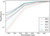 |
Fig. 4 SED of all regions normalised to the flux density in the z′ band. The red, green, blue, cyan and black lines represent respectively the NC, NE, C2, C3 and C5 regions. The dashed lines represent the SED not corrected for the internal extinction whereas the solid lines represent the SED corrected for the extinction assuming a starburst curve (Calzetti 2001) and the extinction values listed in Table 5. Note that the extinguished SEDs of C2 and C5 are similar. |
We see that the tidal features, C2 and C5, have a distinctly different SED, their UV emission being significantly higher relatively to the optical emission compared to other regions. This is most likely due to a combination of several factors. First the interaction triggered a burst of star formation that increases the UV luminosity. The second point is that those tidal features primarily come from the external regions of the galaxies which contain proportionally fewer evolved stars that emit in the optical compared to nuclear regions, this can be seen in Table 3. Conversely, the optical fluxes for regions in the galaxies are enhanced by the photospheric emission of the evolved stellar populations. Finally, as listed in Table 5, the extinction is lower in tidal features compared to more central regions. If we compare C2 and C5 to the extinguished SED, the NE region shows a relatively weak UV emission due to its high extinction enshrouding the nuclear starburst and a strong optical continuum. We see that for the extinction corrected SED, the difference is not as strong compared to the NE clump for instance, showing the importance of the extinction. Finally, NC, the likely host of an AGN, presents a weak UV luminosity with a strong optical emission from old stars.
Beyond the SED, several elements indicate that C5 is a TDG. First of all we see in Fig. 1 that between C4 and C5 there is a faint, extended bridge connecting the two clumps showing the transfer of material from the galaxies to the tip of the tail. This bridge is most likely constituted of evolved stars stripped from the parent galaxies. Unfortunately, the resolution of the HI map does not allow us to evaluate the amount of atomic gas in the bridge. Could it be an interloping object? The optical, HI and CO spectra retrieve a similar recession velocity for C5 showing that the gas and the stars are co-incident. Moreover, the velocity is consistent with the global velocity gradient of the system. This makes it unlikely that C5 is an interloper. Quite evidently, C5 strongly resembles to dwarf galaxies with its relatively low mass, blue colour and low SFR. However, such galaxies generally have a strongly sub-solar metallicity (Tremonti et al. 2004). As we have seen in Sect. 3.2, its metallicity is similar to that of the C2 clump. A possibility would be that these stars actually come from a disrupted low surface brightness galaxy. The interaction could have easily disrupted the baryonic disk. However as we have shown in Sect. 3.5, the virial mass (1.3 × 10⁹ M⊙) is about 3 times that of the visible (HI + H2 + He) mass. Such an interaction would not have been able to destroy the massive dark matter halo of the galaxy. This makes this scenario unlikely. While its high metallicity may be surprising as the interaction strips gas from external regions more easily, the tidal field generates an important mixing of the gas, with the torque injecting lower metallicity gas towards the nucleus, homogeneising the metallicity across the disk (Kewley et al. 2010). A higher metallicity at a given luminosity is one of the best diagnostics to separate dwarf galaxies from recycled objects (Duc & Mirabel 1998). Using the metallicity-luminosity relation for dwarf galaxies of Richer & McCall (1995), C5 would be expected to have 12 + log O/H = 8.1 ± 0.1, much lower than the observed value. Such a discrepancy is expected for collision debris. It appears reasonable that C5 is indeed a TDG rather than a pre-existing object currently undergoing an interaction with the two galaxies.
To gain additional insight, we fit the SED of C5 with an evolutionary synthesis model. It is based on the Pégase ii code (Fioc & Rocca-Volmerange 1997). We consider two populations of arbitrary relative mass: one representing the evolved population stripped from the parent galaxies and the other one the population formed in the TDG. Both populations have an exponentially decreasing SFH. The timescale of the old population is set so that 90% of the original gas reservoir has been transformed into stars by the time of the onset of the formation of the younger component, that is after 12 × 109 years. This timescale is kept as a fixed parameter throughout the fitting procedure. The timescale of the younger population however is a free parameter. Because the dust has only been observed at 24 μm, we do not attempt to fit a dust model to these data as degeneracies would leave dust properties unconstrained. The model is described in much greater detail in Boquien et al. (2010b). Also, the lack of deep enough near-infrared observations does not allow for a precise discussion of the output parameters. Therefore we only use this fit to obtain a new estimate of the SFR with a SFH different than the one assumed by Kennicutt (1998a). The current SFR inferred from the fit is 0.02 M⊙ yr-1, lower than the one calculated from the 24 μm and FUV luminosity, probably reflecting the difference in the assumed star formation history (constant versus exponentially decreasing).
The case of C2 is less evident due to the complexity of the interacting system. It does not seem detached yet from the parent galaxies. The metallicity is slightly lower at 8.61 ± 0.09 which is high enough to rule out a pre-existing dwarf galaxy. An additional hint is given by comparing the UV-to-optical SED of C2 and C5. As we have seen earlier in the present section, they are remarkably similar. The most likely possibility is that this region is the tip of a tidal tail. High resolution HI observations would certainly yield precious information regarding the exact nature of the C2 clump.
4.2. Gas depletion timescale
The gas depletion timescale, which is the time it would take to convert the molecular gas reservoir into stars at the current SFR, can vary between different objects, but it is unclear whether and how it varies within a given interacting system. Braine et al. (2001) showed that collision debris have a depletion timescale of the molecular gas similar to that of spiral galaxies. However, how this timescale changes as a function of the morphology in an interacting system is still an open question. In Table 5 we list the depletion timescale of the molecular gas in the CO(1–0) beams.
The shortest depletion timescale corresponds to the starburst in the eastern nucleus, which is also observed in other nuclear regions. This is expected as starbursts tend to have a shorter depletion timescale (Kennicutt 1998b). The tidal features C3 and C5 show a longer depletion timescale around 2 × 10⁹ yr that is typical of what can be observed in spiral galaxies (Kennicutt 1998b; Bigiel et al. 2011) and in collision debris in general (Braine et al. 2001). C2 however has a shorter depletion timescale. This may be due to an age effect as usual SFR estimators assume a constant SFR which causes an overestimate the current SFR if it is actually declining.
4.3. Schmidt-Kennicutt law
The Schmidt-Kennicutt law links the gas surface density to the SFR surface density:  . Whether and how this law varies is subject of an on-going debate in the literature (Kennicutt 1998b; Gao & Solomon 2004; Kennicutt et al. 2007; Leroy et al. 2008; Bigiel et al. 2008; Blanc et al. 2009; Rahman et al. 2011; Liu et al. 2011). Deviations between quiescent star-forming galaxies and interacting systems can have important implications regarding our understanding of galaxy formation and evolution. The fundamental reason is that the ISM (interstellar medium) of high redshift galaxies is turbulent (Förster Schreiber et al. 2006), and that they are gas rich (Tacconi et al. 2010; Daddi et al. 2010). Nearby interacting systems, by having an enhanced turbulence, can be seen as analogues of high redshift galaxies. Recent high resolution simulations by Teyssier et al. (2010) show that interacting galaxies deviate from the standard Schmidt-Kennicutt law seen in spiral disks, which could be explained by the effect of gas turbulence and fragmentation. Whether star formation proceeds similarly to the Schmidt-Kennicutt law in local interacting galaxies is therefore important to gain insight into the mode of star formation at high redshift.
In a first step we examine how the molecular hydrogen column density and the SFR surface density in the different regions in Arp 158 compare to the relation derived by Bigiel et al. (2008) in the case of spiral galaxies. The SFR in Arp 158 corresponds to the 24+FUV measurement in Table 5 which is the same to that used by Bigiel et al. (2008).
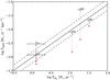 |
Fig. 5 SFR surface density versus the molecular hydrogen surface density. The points with the 3-σ error bars represent pointings in the Arp 158 system with the SFR derived from the FUV + 24 μm relation, and the red circles adopt the SFR derived from the fit of the SED assuming the burst has the extinction calculated in Table 5. The solid black line represents the Schmidt-Kennicutt law for molecular hydrogen derived by Bigiel et al. (2008) for spiral galaxies: log ΣSFR = −3.02 + 0.96log ΣH2, with ΣSFR in M⊙ yr-1 kpc-2 and ΣH2 in M⊙ pc-2. The dashed lines represent the typical 0.2 dex scatter. The molecular mass does not take into account the helium contribution in any case. |
Even though there are only a few measurements, the SFR and the H2 surface densities span more than one order of magnitude and are well correlated with each other in Arp 158. The NC, C3 and C5 regions follow the same relation as spiral galaxies, which is consistent with the results found by Braine et al. (2001) on TDG. The NE and C2 regions exhibit clear excesses of their SFR in comparison to their molecular gas surface density. This is easily explainable for NE as it is a nuclear starburst. This finding confirms observational and theoretical results for starburst galaxies. Another possibility for NE and C2 is that the molecular gas is more concentrated than star formation so that averaging over the beam would underestimate the molecular gas surface density. However, if the gas and star formation are equally extended it would move the points mostly parallel to the Bigiel et al. (2008) relation. Interferometric observations of the entire system would be required to answer this question. Another possibility is that a strong burst quickly depleted the molecular gas reservoir or that star formation tracers give a significantly overevaluated SFR. In all cases, if the burst SFH is decreasing, the standard SFR estimators which assume a constant SFR over 100 Myr will likely overestimate the actual SFR. As star-formation in collision debris tends to be more bursty compared to star-formation averaged over a galactic disk, this could artificially enhance the derived SFR in these regions. When using the SFR derived from the SED fitting we notice that NE and C2 are not strongly deviant anymore compared to the other regions. This shows that great caution must be employed to estimate the SFR as it can influence the results significantly, especially in the case of interacting systems in which the actual SFR can vary rapidly.
As mentioned earlier, Daddi et al. (2010) found that starburst galaxies follow a different Schmidt-Kennicutt law than more quiescent galaxies. The interaction in Arp 158 increases the turbulence in the system. The question is whether different regions in the system also follow different relations. In Fig. 6, we compare the regions in Arp 158 with the relations found by Daddi et al. (2010).
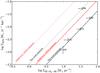 |
Fig. 6 SFR surface density versus the gas surface density, including HI, H2 and He. The points with the 3-σ error bars represent pointings in the Arp 158 system. To take He into account we have multiplied the H2 column density by a factor 1.38. As the HI resolution is significantly worse than the CO beam size, we have used the column density in the central pixel as listed in Table 6. The actual column density remains uncertain and requires higher resolution HI observations. The solid red line represents Daddi et al. (2010) relation derived for BzK galaxies: log ΣSFR = −3.83 + 1.42log Σgas, with ΣSFR in M⊙ yr-1 kpc-2 and Σgas in M⊙ pc-2. The dotted red line is the same relation offset by 0.9 dex fitting ULIRGs. The Daddi et al. (2010) relation has been converted from a Chabrier (2003) IMF to a Kroupa (2001) one for easier comparison. The solid black line represents the best fit for the Arp 158 apertures excluding NE with the same slope as the Daddi et al. (2010) relation. Finally the dotted black line represents the same relation offset to pass through the NE region. |
We see that similarly to what Daddi et al. (2010) found, we are seeing 2 different regimes of star formation in Arp 158, provided the SFR estimator is accurate. The first one regroups all regions, except for NE, which are well fitted by a power law with a slope of 1.42. Conversely NE presents a much higher SFR surface density for a similar surface density, with an offset which is qualitatively similar to the one found by Daddi et al. (2010) for starburst galaxies. The offset is slightly larger in the case of Daddi et al. (2010), probably as the objects they studied are more extreme than ours. Another important point is that contrary to Daddi et al. (2010) we find this offset while keeping the XCO conversion factor constant. Using a smaller conversion factor similar to that used for LIRGs and ULIRGs would only increase the discrepancy. What really sets NE apart is not the gas surface density but the high SFR surface density. A possible explanation is that this region is not simply an inflow-driven starburst but that the increased turbulence and a fragmentation into dense clouds strongly increase the SFR surface density for the same gas surface density (Teyssier et al. 2010; Bournaud et al. 2010b, 2011). An observational signature of this would be an an excess of the dense gas fraction as observed by Juneau et al. (2009). In order to determine whether the dense gas fraction is higher, some HCN observations are required. We stress that the use of a lower XCO factor, as is used for ULIRGs for instance, for the NE region would only exacerbate the discrepancy.
The presence of these 2 modes seen in a resolved way in an interacting system shows that its origin does not depend on the global mass or size of the system but that it is rather linked to the physics of the ISM at scales no larger than 1 kpc. Indeed, this scale corresponds to the largest gravitational instabilities in the ISM. The Jeans length which is of the order of 100–200 pc in nearby spirals increases up to 500–1000 pc in mergers because of higher densities and velocity dispersions. In addition this scale also corresponds to the injection scale of turbulence in the ISM (Elmegreen et al. 2003; Bournaud et al. 2010a).
5. Summary and conclusion
In this paper we have studied how properties of star-forming regions vary across an interacting system. To do so we have combined an extensive set of archival and proprietary data tracing the molecular gas (CO), the atomic gas (HI), star formation (FUV and 24 μm), and the stellar populations. The interacting system shows a complex morphology, the disks of the 2 colliding galaxies having already interpenetrated. To ascertain the exact nature of the different regions in the interacting system we have also obtained optical spectra. In particular we have obtained a firm identification of the nuclei of the merging galaxies, which was still under debate. One, to the east, exhibits a starburst, the other one hosts an AGN. A third nucleus, to the west, turns out to be a foreground star. A brief description of the regions of interest in Arp 158 is provided hereafter.
-
NE: The emission of the eastern nucleus is peaked and is strong at24 μm, suggesting an AGN or a nuclear starburst. The emission line ratios from the BPT diagram (Baldwin et al. 1981) show that it is most likely the latter. The starburst is probably due to gas losing angular momentum as a result of the interaction, and inflowing towards the centre of the galaxy as a consequence.
-
NC: Emission line ratios of the central nucleus hint at an AGN, either an extreme LINER or a Seyfert. This unfortunately compromises any accurate measure of the SFR in this regions.
-
NW: Optical spectroscopy clearly shows that this is a foreground star with a strong Hα Balmer line in absorption at zero velocity. A faint Hα emission at the redshift of the system is also observed showing that the star may mask a star-forming region. A close inspection of 2MASS near-infrared images also shows that NW is qualitatively more compact than NC and NE. This confirms what Chincarini & Heckathorn (1973) found and closes the question of the nature of this object.
-
C1: A peak is visible at 24 μm without counterpart in ultraviolet, hinting that it may be a young, dusty star-forming region that has yet to break the surrounding dust cloud. The CO emission of this clump is encompassed by the CO(1–0) beam for the NC pointing.
-
C2: The western tip of the system is peaked at 24 μm with a faint counterpart in the ultraviolet. CO observations show that it is only marginally detected in CO(1–0) and not detected in CO(2–1), with a detection threshold at 3-σ.
-
C3: The region is particularly peaked in FUV and NUV but does not present a similar peak at 24 μm. However CO emission is clearly detected.
-
C4: A faint 24 μm peak can be seen without any counterpart in the ultraviolet showing the possible presence of embedded star-forming regions. The NE CO pointing overlaps partially with this region in CO(1–0).
-
C5: The TDG candidate is clearly peaked in both the 24 μm and the ultraviolet bands. A faint, diffuse UV emission can be seen in the bridge linking it to the main bodies of the interaction. CO observations show a clear detection both in CO(1–0) and in CO(2–1).
Studying the Schmidt-Kennicutt law, most regions in the system follow closely the relation found in spiral galaxies by Bigiel et al. (2008), with the exception of the nuclear starburst and the tip of one of the tidal tails which show a significantly larger efficiency. Comparisons with the relations derived by Daddi et al. (2010) exhibit the presence of 2 star formation modes. The detection of these 2 modes in a resolved way hints that their origin is linked to the physics of the interstellar medium at scales no larger than 1 kpc, the size of the largest gravitational instabilities and the injection scale of turbulence.
Value obtained from NED, the NASA Extragalactic Database operated by the Jet Propulsion Laboratory, California Institute of Technology, under contract with the National Aeronautics and Space Administration.
Acknowledgments
We would like to thank the anonymous referee for his/her useful comments that have helped improve this paper. We would like to thank Caroline Simpson for kindly providing the HI data for the Arp 158 system. We thank the William Herschel Telescope staff for carrying out the spectroscopic observations in service mode. We also thank the IRAM staff for carrying out part of the CO observations in service mode. UL acknowledges financial support from the research grants AYA2007-67625-C02-02 from the Spanish Ministerio de Ciencia y Educación and FQM-0108 from the Junta de Andalucía (Spain). U.L. warmly thanks IPAC (Caltech), where most of this work was done during a sabbatical stay, for their hospitality. V.C. would like to acknowledge partial support from the E.U. grant FP7-REGPOT 206469. This research has made use of the NASA/IPAC Extragalactic Database (NED) which is operated by the Jet Propulsion Laboratory, California Institute of Technology, under contract with the National Aeronautics and Space Administration.
References
- Abazajian, K. N., Adelman-McCarthy, J. K., Agüeros, M. A., et al. 2009, ApJS, 182, 543 [NASA ADS] [CrossRef] [Google Scholar]
- Baldwin, J. A., Phillips, M. M., & Terlevich, R. 1981, PASP, 93, 5 [NASA ADS] [CrossRef] [EDP Sciences] [Google Scholar]
- Barnes, J. E. 2004, MNRAS, 350, 798 [NASA ADS] [CrossRef] [Google Scholar]
- Bigiel, F., Leroy, A., Walter, F., et al. 2008, AJ, 136, 2846 [NASA ADS] [CrossRef] [Google Scholar]
- Bigiel, F., Leroy, A. K., Walter, F., et al. 2011, ApJ, 730, L13 [NASA ADS] [CrossRef] [Google Scholar]
- Blanc, G. A., Heiderman, A., Gebhardt, K., Evans, N. J., & Adams, J. 2009, ApJ, 704, 842 [NASA ADS] [CrossRef] [Google Scholar]
- Boquien, M., Duc, P.-A., Braine, J., et al. 2007, A&A, 467, 93 [NASA ADS] [CrossRef] [EDP Sciences] [Google Scholar]
- Boquien, M., Duc, P., Wu, Y., et al. 2009, AJ, 137, 4561 [NASA ADS] [CrossRef] [Google Scholar]
- Boquien, M., Bendo, G., Calzetti, D., et al. 2010a, ApJ, 713, 626 [NASA ADS] [CrossRef] [Google Scholar]
- Boquien, M., Duc, P., Galliano, F., et al. 2010b, AJ, 140, 2124 [NASA ADS] [CrossRef] [Google Scholar]
- Bournaud, F., Duc, P.-A., Amram, P., Combes, F., & Gach, J.-L. 2004, A&A, 425, 813 [NASA ADS] [CrossRef] [EDP Sciences] [Google Scholar]
- Bournaud, F., Duc, P.-A., Brinks, E., et al. 2007, Science, 316, 1166 [NASA ADS] [CrossRef] [PubMed] [Google Scholar]
- Bournaud, F., Elmegreen, B. G., Teyssier, R., Block, D. L., & Puerari, I. 2010a, MNRAS, 409, 1088 [NASA ADS] [CrossRef] [Google Scholar]
- Bournaud, F., Powell, L. C., Chapon, D., & Teyssier, R. 2010b [arXiv:1012.5227] [Google Scholar]
- Bournaud, F., Chapon, D., Teyssier, R., et al. 2011, ApJ, 730, 4 [NASA ADS] [CrossRef] [Google Scholar]
- Braine, J., & Combes, F. 1992, A&A, 264, 433 [NASA ADS] [Google Scholar]
- Braine, J., Lisenfeld, U., Duc, P.-A., & Leon, S. 2000, Nature, 403, 867 [NASA ADS] [CrossRef] [PubMed] [Google Scholar]
- Braine, J., Duc, P.-A., Lisenfeld, U., et al. 2001, A&A, 378, 51 [NASA ADS] [CrossRef] [EDP Sciences] [Google Scholar]
- Braine, J., Lisenfeld, U., Duc, P., et al. 2004, A&A, 418, 419 [NASA ADS] [CrossRef] [EDP Sciences] [Google Scholar]
- Braine, J., Gratier, P., Kramer, C., et al. 2010, A&A, 520, A107 [Google Scholar]
- Buat, V., Iglesias-Páramo, J., Seibert, M., et al. 2005, ApJ, 619, L51 [NASA ADS] [CrossRef] [Google Scholar]
- Calzetti, D. 1997, AJ, 113, 162 [NASA ADS] [CrossRef] [Google Scholar]
- Calzetti, D. 2001, PASP, 113, 1449 [NASA ADS] [CrossRef] [Google Scholar]
- Calzetti, D., Kennicutt, R. C., Engelbracht, C. W., et al. 2007, ApJ, 666, 870 [NASA ADS] [CrossRef] [Google Scholar]
- Calzetti, D., Wu, S., Hong, S., et al. 2010, ApJ, 714, 1256 [NASA ADS] [CrossRef] [Google Scholar]
- Cardelli, J. A., Clayton, G. C., & Mathis, J. S. 1989, ApJ, 345, 245 [NASA ADS] [CrossRef] [Google Scholar]
- Chabrier, G. 2003, PASP, 115, 763 [NASA ADS] [CrossRef] [Google Scholar]
- Chien, L., & Barnes, J. E. 2010, MNRAS, 407, 43 [NASA ADS] [CrossRef] [MathSciNet] [Google Scholar]
- Chincarini, G., & Heckathorn, H. M. 1973, PASP, 85, 568 [NASA ADS] [CrossRef] [Google Scholar]
- Cortese, L., Gavazzi, G., Boselli, A., et al. 2006, A&A, 453, 847 [Google Scholar]
- Daddi, E., Elbaz, D., Walter, F., et al. 2010, ApJ, 714, L118 [Google Scholar]
- Dahari, O. 1985, ApJS, 57, 643 [NASA ADS] [CrossRef] [Google Scholar]
- Dale, D. A., & Helou, G. 2002, ApJ, 576, 159 [NASA ADS] [CrossRef] [Google Scholar]
- Denicoló, G., Terlevich, R., & Terlevich, E. 2002, MNRAS, 330, 69 [NASA ADS] [CrossRef] [Google Scholar]
- Duc, P.-A. 1995, Ph.D. Thesis, Université Paris VI [Google Scholar]
- Duc, P.-A., & Mirabel, I. F. 1998, A&A, 333, 813 [NASA ADS] [Google Scholar]
- Duc, P.-A., Brinks, E., Springel, V., et al. 2000, AJ, 120, 1238 [NASA ADS] [CrossRef] [Google Scholar]
- Duc, P.-A., Braine, J., Lisenfeld, U., Brinks, E., & Boquien, M. 2007, A&A, 475, 187 [NASA ADS] [CrossRef] [EDP Sciences] [Google Scholar]
- Elmegreen, B. G., Elmegreen, D. M., & Leitner, S. N. 2003, ApJ, 590, 271 [NASA ADS] [CrossRef] [Google Scholar]
- Fioc, M., & Rocca-Volmerange, B. 1997, A&A, 326, 950 [NASA ADS] [Google Scholar]
- Förster Schreiber, N. M., Genzel, R., Lehnert, M. D., et al. 2006, ApJ, 645, 1062 [NASA ADS] [CrossRef] [Google Scholar]
- Gao, Y., & Solomon, P. M. 2004, ApJ, 606, 271 [NASA ADS] [CrossRef] [Google Scholar]
- Gardan, E., Braine, J., Schuster, K. F., Brouillet, N., & Sievers, A. 2007, A&A, 473, 91 [NASA ADS] [CrossRef] [EDP Sciences] [Google Scholar]
- Genzel, R., Tacconi, L. J., Gracia-Carpio, J., et al. 2010, MNRAS, 407, 2091 [NASA ADS] [CrossRef] [Google Scholar]
- Gerhard, O., Arnaboldi, M., Freeman, K. C., & Okamura, S. 2002, ApJ, 580, L121 [NASA ADS] [CrossRef] [Google Scholar]
- Gratier, P., Braine, J., Rodriguez-Fernandez, N. J., et al. 2010, A&A, 522, A3 [NASA ADS] [CrossRef] [EDP Sciences] [Google Scholar]
- Hancock, M., Smith, B. J., Struck, C., et al. 2007, AJ, 133, 676 [NASA ADS] [CrossRef] [Google Scholar]
- Hancock, M., Smith, B. J., Struck, C., Giroux, M. L., & Hurlock, S. 2009, AJ, 137, 4643 [NASA ADS] [CrossRef] [Google Scholar]
- Iyer, M. G., Simpson, C. E., Gottesman, S. T., & Malphrus, B. K. 2004, AJ, 128, 985 [NASA ADS] [CrossRef] [Google Scholar]
- Juneau, S., Narayanan, D. T., Moustakas, J., et al. 2009, ApJ, 707, 1217 [NASA ADS] [CrossRef] [Google Scholar]
- Kennicutt, Jr., R. C. 1998a, ARA&A, 36, 189 [Google Scholar]
- Kennicutt, Jr., R. C. 1998b, ApJ, 498, 541 [NASA ADS] [CrossRef] [Google Scholar]
- Kennicutt, Jr., R. C., Calzetti, D., Walter, F., et al. 2007, ApJ, 671, 333 [NASA ADS] [CrossRef] [Google Scholar]
- Kewley, L. J.,Rupke, D., Jabran Zahid, H., Geller, M. J., & Barton, E. J. 2010, ApJ, 721, L48 [NASA ADS] [CrossRef] [Google Scholar]
- Kroupa, P. 2001, MNRAS, 322, 231 [NASA ADS] [CrossRef] [Google Scholar]
- Leroy, A., Bolatto, A., Walter, F., & Blitz, L. 2006, ApJ, 643, 825 [NASA ADS] [CrossRef] [Google Scholar]
- Leroy, A. K., Walter, F., Brinks, E., et al. 2008, AJ, 136, 2782 [NASA ADS] [CrossRef] [Google Scholar]
- Lisenfeld, U., Braine, J., Duc, P.-A., et al. 2002, A&A, 394, 823 [NASA ADS] [CrossRef] [EDP Sciences] [Google Scholar]
- Lisenfeld, U., Braine, J., Duc, P.-A., et al. 2004, A&A, 426, 471 [NASA ADS] [CrossRef] [EDP Sciences] [Google Scholar]
- Liu, G., Koda, J., Calzetti, D., Fukuhara, M., & Momose, R. 2011, ApJ, 735, 63 [NASA ADS] [CrossRef] [Google Scholar]
- Mendes de Oliveira, C.,Cypriano, E. S.,Sodré, Jr., L., & Balkowski, C. 2004, ApJ, 605, L17 [NASA ADS] [CrossRef] [Google Scholar]
- Petitpas, G. R., & Taylor, C. L. 2005, ApJ, 633, 138 [NASA ADS] [CrossRef] [Google Scholar]
- Rahman, N., Bolatto, A. D., Wong, T., et al. 2011, ApJ, 730, 72 [NASA ADS] [CrossRef] [Google Scholar]
- Relaño, M., Lisenfeld, U., Pérez-González, P. G., Vílchez, J. M., & Battaner, E. 2007, ApJ, 667, L141 [NASA ADS] [CrossRef] [Google Scholar]
- Richer, M. G., & McCall, M. L. 1995, ApJ, 445, 642 [NASA ADS] [CrossRef] [Google Scholar]
- Ryan-Weber, E. V., Meurer, G. R., Freeman, K. C., et al. 2004, AJ, 127, 1431 [NASA ADS] [CrossRef] [Google Scholar]
- Sakai, S.,Kennicutt, Jr., R. C., van der Hulst, J. M., & Moss, C. 2002, ApJ, 578, 842 [NASA ADS] [CrossRef] [Google Scholar]
- Sauvage, M., & Thuan, T. X. 1992, ApJ, 396, L69 [NASA ADS] [CrossRef] [Google Scholar]
- Schmidt, M. 1959, ApJ, 129, 243 [NASA ADS] [CrossRef] [Google Scholar]
- Skrutskie, M. F., Cutri, R. M., Stiening, R., et al. 2006, AJ, 131, 1163 [NASA ADS] [CrossRef] [Google Scholar]
- Solomon, P. M., & Van den Bout, P. A. 2005, ARA&A, 43, 677 [NASA ADS] [CrossRef] [Google Scholar]
- Tacconi, L. J., Genzel, R., Neri, R., et al. 2010, Nature, 463, 781 [Google Scholar]
- Teyssier, R., Chapon, D., & Bournaud, F. 2010, ApJ, 720, L149 [NASA ADS] [CrossRef] [Google Scholar]
- Toomre, A. 1977, in Evolution of Galaxies and Stellar Populations, ed. B. M. Tinsley, & R. B. Larson, 401 [Google Scholar]
- Tremonti, C. A., Heckman, T. M., Kauffmann, G., et al. 2004, ApJ, 613, 898 [NASA ADS] [CrossRef] [Google Scholar]
- Weilbacher, P. M.,Duc, P.-A., & Fritze-v. Alvensleben, U. 2003, A&A, 397, 545 [NASA ADS] [CrossRef] [EDP Sciences] [Google Scholar]
- Werk, J. K., Putman, M. E., Meurer, G. R., et al. 2008, ApJ, 678, 888 [NASA ADS] [CrossRef] [Google Scholar]
- Werk, J. K., Putman, M. E., Meurer, G. R., et al. 2010, AJ, 139, 279 [NASA ADS] [CrossRef] [Google Scholar]
- Wilson, T. L., Rohlfs, K., & Hüttemeister, S. 2009, Tools of Radio Astronomy, ed. T. L. Wilson, K. Rohlfs, & S. Hüttemeister (Springer-Verlag) [Google Scholar]
- Yoshida, M., Yagi, M., Okamura, S., et al. 2002, ApJ, 567, 118 [NASA ADS] [CrossRef] [Google Scholar]
All Tables
All Figures
|
Fig. 1 Top: optical image in g′ (blue channel), r′ (green channel) and i′ (red channel) bands. The regions of interest listed in Table 1 are indicated with a red label. The white dashed rectangles represent the two long slits used for optical spectroscopy. Bottom: FUV (blue channel), NUV (green channel) and 24 μm (red channel). The contours in cyan trace the HI column density. The yellow dashed circles represent the CO(1–0) beams and the area in which fluxes have been measured. Due to the large CO beams, not all regions of interest can have their CO emission detected separately. |
| In the text | |
|
Fig. 2 Left: blue part of the spectrum of the NE clump. Several lines are clearly detected: [OII] 372.7, Hγ, [OIII] 436.3, Hβ, [OIII] 495.9, and [OIII] 500.7. Unfortunately the blue spectrum for other clumps is not deep enough to detect these emission lines. Right: spectra of clumps NE, NC, NW, C2, and C5. The spectra have been offset to distinguish them more easily. The spectra of clumps NC, NW, C2, and C5 are multiplied by 5 as they are intrinsically much fainter than the spectrum of NE. Except for NW, several lines are clearly detected: [NII] 654.8, Hα, [NII] 658.4, [SII] 671.7, and [SII] 673.1. The spectrum of NW shows a broad Hα line in absorption at almost 0-velocity with a weak Hα emission line at the recession velocity of Arp 158. |
| In the text | |
|
Fig. 3 Spectra of the five regions. CO(1–0) is shown in black, CO(2–1) in green, and HI in red. The HI spectra correspond to the central pixel in the CO beam in order to limit the blending with adjacent sources. We have multiplied the flux of the CO spectra by 5 in the case of C2 and C5 to make them more visible. All spectra have been centred to a velocity of 4800 km s-1. |
| In the text | |
|
Fig. 4 SED of all regions normalised to the flux density in the z′ band. The red, green, blue, cyan and black lines represent respectively the NC, NE, C2, C3 and C5 regions. The dashed lines represent the SED not corrected for the internal extinction whereas the solid lines represent the SED corrected for the extinction assuming a starburst curve (Calzetti 2001) and the extinction values listed in Table 5. Note that the extinguished SEDs of C2 and C5 are similar. |
| In the text | |
|
Fig. 5 SFR surface density versus the molecular hydrogen surface density. The points with the 3-σ error bars represent pointings in the Arp 158 system with the SFR derived from the FUV + 24 μm relation, and the red circles adopt the SFR derived from the fit of the SED assuming the burst has the extinction calculated in Table 5. The solid black line represents the Schmidt-Kennicutt law for molecular hydrogen derived by Bigiel et al. (2008) for spiral galaxies: log ΣSFR = −3.02 + 0.96log ΣH2, with ΣSFR in M⊙ yr-1 kpc-2 and ΣH2 in M⊙ pc-2. The dashed lines represent the typical 0.2 dex scatter. The molecular mass does not take into account the helium contribution in any case. |
| In the text | |
|
Fig. 6 SFR surface density versus the gas surface density, including HI, H2 and He. The points with the 3-σ error bars represent pointings in the Arp 158 system. To take He into account we have multiplied the H2 column density by a factor 1.38. As the HI resolution is significantly worse than the CO beam size, we have used the column density in the central pixel as listed in Table 6. The actual column density remains uncertain and requires higher resolution HI observations. The solid red line represents Daddi et al. (2010) relation derived for BzK galaxies: log ΣSFR = −3.83 + 1.42log Σgas, with ΣSFR in M⊙ yr-1 kpc-2 and Σgas in M⊙ pc-2. The dotted red line is the same relation offset by 0.9 dex fitting ULIRGs. The Daddi et al. (2010) relation has been converted from a Chabrier (2003) IMF to a Kroupa (2001) one for easier comparison. The solid black line represents the best fit for the Arp 158 apertures excluding NE with the same slope as the Daddi et al. (2010) relation. Finally the dotted black line represents the same relation offset to pass through the NE region. |
| In the text | |
Current usage metrics show cumulative count of Article Views (full-text article views including HTML views, PDF and ePub downloads, according to the available data) and Abstracts Views on Vision4Press platform.
Data correspond to usage on the plateform after 2015. The current usage metrics is available 48-96 hours after online publication and is updated daily on week days.
Initial download of the metrics may take a while.