| Issue |
A&A
Volume 531, July 2011
|
|
|---|---|---|
| Article Number | A29 | |
| Number of page(s) | 9 | |
| Section | Planets and planetary systems | |
| DOI | https://doi.org/10.1051/0004-6361/201116510 | |
| Published online | 06 June 2011 | |
Modeling the radio signature of the orbital parameters, rotation, and magnetic field of exoplanets
1 LASP, University of Colorado at Boulder, USA
2
LESIA, Observatoire de Paris CNRS, UPMC, Univ. Paris 7, France
e-mail: This email address is being protected from spambots. You need JavaScript enabled to view it.
3
LATMOS-IPSL, Université Versailles St.-Quentin, CNRS/INSU, France
e-mail: This email address is being protected from spambots. You need JavaScript enabled to view it.
Received: 14 January 2011
Accepted: 16 March 2011
Abstract
Context. Since the first extra-solar planet discovery in 1995, several hundreds of these planets have been discovered. Most are hot Jupiters, i.e. massive planets orbiting close to their star. These planets may be powerful radio emitters.
Aims. We simulate the radio dynamic spectra resulting from various interaction models between an exoplanet and its parent star, i.e. exoplanet-induced stellar emission and three variants of the exoplanet’s magnetospheric auroral radio emission (full auroral oval, active sector fixed in longitude, and active sector fixed in local time).
Methods. We show the physical information about the system that can be drawn from radio observations, and how this can be achieved. This information includes the magnetic field strength and the rotation period of the emitting body (planet or star), the orbital period, the orbit’s inclination, and the magnetic field tilt relative to the rotation axis or offset relative to the center of the planet. For most of these parameters, radio observations provide a unique means of measuring them.
Results. Our results should provide the proper framework of analysis and interpretation for future detections of radio emissions from exoplanetary systems – or from magnetic white dwarf-planet or white dwarf-brown dwarf systems –, that are expected to commence soon as part of extensive programs at large radiotelescopes such as LOFAR, UTR2 or the GMRT. Our methodology can be easily adapted to simulate specific observations, once effective detection is achieved.
Key words: planet-star interactions / planets and satellites: aurorae / radio continuum: planetary systems
© ESO, 2011
1. Introduction
The relatively high contrast (~1 in our Solar System) between planetary and solar low frequency radio emission suggests that the low frequency radio range may be the most suitable for the direct detection and study of exoplanets using large ground-based radiotelescopes (Zarka 2007, and references therein). The spectral range of interest is typically between ~10 MHz (the Earth’s ionospheric cutoff) and a few tens of MHz (the natural upper limit to the planetary radio emission, 40 MHz in the case of Jupiter). Searches for exoplanetary radio signals have been or are presently performed at the VLA at 74 MHz (see e.g. Lazio & Farrell 2007), at the GMRT at 150 MHz (Winterhalter et al. 2006), 244 and 614 MHz (Lecavelier Des Etangs et al. 2009), and with the UTR2 radiotelescope (Ryabov et al. 2004; Zarka 2007, 2010). Although no detection has been made yet, theoretical estimates predict, especially for hot Jupiters (Zarka 2004a, 2007; Grießmeier et al. 2007), but also for planets orbiting at several AU from their parent star (Nichols 2011), that the flux densities are 104 − 6 times higher than that of Jupiter (i.e. of the order of 1 Jy with ~1 MHz × 1 min integration), thus near the detection limit of the largest existing radiotelescopes or the new facilities soon in operation such as LOFAR (Fender et al. 2006) and the LWA (Ellingson et al. 2009).
The motivations for the radio detection and study of exoplanets are diverse. Besides directly detecting exoplanetary photons and vastly expanding the field of comparative magnetospheric physics to star-planet plasma interactions in general, cyclotron radio emission is expected to provide measurements or estimates of fundamental planetary physical properties such as: the planet’s surface magnetic field, placing constraints on internal structure models (Sánchez-Lavega 2004), and empirical scaling laws for planetary magnetic fields (see e.g. Farrell et al. 1999); the planetary rotation period, which can be independently deduced from the rotational modulation of the radio emission, permitting us to check whether the planet is tidally spin-orbit locked; and the orbit inclination, which might be deduced from the comparison of the emission diagrams originating from the two hemispheres.
These expectations are directly based on our knowledge of the phenomenology of Solar system planetary radio emissions (see e.g. Zarka 1998, 2000, 2004b). However, it is interesting to quantitatively test, by means of the realistic modeling of the expected emission’s source distribution and beaming, how and to what extent these important parameters could be deduced from true detections and observations of exoplanetary radio emissions, expected to occur in the near future.
Until now, modeling and extrapolations of Solar system scaling laws (Zarka et al. 2001; Zarka 2007; Grießmeier et al. 2007; Nichols 2011, and references therein) have been made to predict reasonable orders of magnitudes for the intensity of exoplanetary radio emissions, demonstrating the interest in attempting their detection. However, these works did not address the characteristics of the expected radio signal, such as its polarization, time-frequency distribution, or modulations. Since 2008, we have developed a simulation tool to allow us to successfully compute intensity and polarization dynamic spectra of Jupiter’s and Saturn’s non-thermal radio emission (Hess et al. 2008a; Lamy et al. 2008a). This tool has been named ExPRES (Exoplanetary and Planetary Radio Emissions Simulator). From physically sound assumptions about the radiosource distribution and beaming in the planetary environment (generally at high latitudes), based on a planetary magnetic field model and the physics of the cyclotron-maser instability (CMI), which is known to cause the intense planetary auroral and satellite-induced radio emission (Wu 1985; Treumann 2006), this software can compute the intensity and polarization dynamic spectra that would be measured by a fixed or mobile (e.g. orbiting) observer.
Since any exoplanetary radio sources could not be resolved spatially, the relevant observations that we expect to obtain are time-frequency distributions of intensity and polarization (so-called dynamic spectra), as modeled by ExPRES. In the present paper, we perform and analyze ExPRES simulations of the two types of high-latitude cyclotron radio emission observed in our solar system and discussed in Zarka (2007): the ubiquitous auroral magnetospheric radio emission from all magnetized planets, generated by magnetosphere-solar wind interaction, and the emission produced by satellite-planet electrodynamic interactions. The former case corresponds to the interaction of a weakly magnetized flow (the solar wind) with a strongly magnetized (planetary) obstacle, while the latter corresponds to the interaction of a strongly magnetized flow (the magnetospheric plasma) with a magnetized obstacle (via magnetic reconnection, e.g. at Ganymede) or an unmagnetized obstacle (via generation of Alfvén waves and currents, e.g. at Io). As for exoplanets, we expect to detect either auroral emission from the exoplanetary magnetosphere itself (if the exoplanet is strongly magnetized), or emission induced by the exoplanet through interaction with the stellar magnetic field (as a giant analog of the satellite-Jupiter case) regardless of whether the exoplanet is magnetized or not. The latter case also applies to the magnetic white dwarf-planet or white dwarf-brown dwarf systems studied in the literature (Willes & Wu 2004, 2005).
Previous studies have found that in our Solar system, the dissipated power is always a nearly constant fraction of the flow’s electromagnetic (Poynting) flux on the obstacle 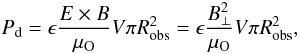 (1)where V is the flow speed and ϵ an efficiency factor of ~ 0.2 ± 0.1. Even more remarkably, the resulting radio power has been found to be a nearly constant fraction (1–5%) of the dissipated power, thus a nearly constant fraction (η = 2 − 10 × 10-3) of the flow’s Poynting flux (Zarka et al. 2001; Zarka 2007, and references therein). Applying these results to known exoplanets, hot Jupiters are found to be the most likely sources of any detectable radio emission, either in their magnetosphere if the planetary surface magnetic field exceeds a few gauss (1 G = 10-4 T), hereafter called exoplanetary radio emission –, and/or in the parent star’s corona near the sub-planetary point if the stellar magnetic field exceeds several tens of gauss (Zarka 2007; Grießmeier et al. 2007), hereafter called stellar (exoplanet-induced) radio emission.
It would not be possible to simulate all the possible cases of field strength, topology and rotation periods of both the exoplanet and its parent star, of orbital period and inclination of the exoplanet, of type of generation scenario (exoplanetary or stellar), radio source distribution and beaming. The purpose of this paper is thus to discuss prototype ExPRES simulations of generic/typical cases to show which parameters can be deduced from the future intensity and polarization dynamic spectra, and how they can be derived, identifying possible degeneracies). This will set the framework for first comparisons to actual detections as well as future ExPRES simulations intended to model accurately the measured dynamic spectra. The generic cases chosen here correspond to two models of interactions:
-
stellar radio emission, i.e an exoplanet-induced – Io-like – hotspot near the star at the sub-planetary point;
-
exoplanetary auroral radio emissions, including:
-
emission along a full auroral oval;
-
emission along a restricted sector of “active” longitudes, i.e. Jupiter-like;
-
emission along a sector of “active” local time, i.e. Saturn- or Earth-like.
-
The stellar or planetary magnetic field are assumed to be dipolar, either axisymmetric or tilted (by 15°) relative to the body’s rotation axis, itself perpendicular to the planetary orbital plane. The maximum cyclotron frequency is arbitrarily set to fce = eB/2πme = 38 MHz at the footprint of the L = 20 field line (by analogy with the case of Jupiter). An inclination i of the exoplanetary orbit as seen by the terrestrial observer between 0° and 90° (in steps of 15°) is considered. Here i = 0° corresponds to the observer being in the orbital plane of the planet, and i = 90° corresponds to an orbital plane in the plane of the sky. Our discussion here focuses on the 0° and 15° representative cases. The low frequency cutoff (occultation) of the observed radio emission by the circumstellar plasma envelope – assumed to be spherical – is taken into account (and assumed to occur at the local plasma frequency fpe). Finally, values for the planetary orbital, stellar rotation, and planetary rotation periods are set to the values Porb = 2 × 10⁴ min ≃ 13.9 days, Prot - planet = 8 × 10³ min ≃ 5.6 days = Porb/2.5, and Prot - star = 4.444 × 10³ min ≃ 3.1 days = Porb/4.5. We arbitrarily ordered these values as Porb > Prot - planet > Prot - star and avoided there being integer ratios between them. Alternative orders probably exist in the known exoplanetary systems that can be easily modelled.
In Sect. 2, we briefly summarize the physics of electron acceleration and radio emission in Solar System planets’ magnetospheres. In Sect. 3, we then present the ExPRES code and its underlying physical assumptions. Section 4 describes the simulation results for stellar radio emission (Sect. 4.1) and exoplanet-induced radio emission (Sect. 4.2). These simulation results are then discussed to help us discriminate between the two interaction models (Sect. 5) and determine planetary physical and orbital parameters (Sect. 6). We finally synthesize our results and discuss possible extensions of this work in Sect. 7.
2. Planetary radio emission and electron acceleration
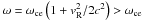
Electrons with energies of a few keV are observed in high latitude regions of all planetary magnetospheres. These electrons are the source of radio emission generated at the local fce. An in situ exploration of Earth’s auroral regions has permitted us to identify the CMI as the generation mechanism for radio waves, based on resonance between a circularly polarized wave and the gyration motion of electrons in the planet’s magnetic field (Wu 1985; Treumann 2006). The resonance condition is given by 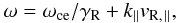 (2)where ωce = 2πfce, γR is the Lorentz factor or resonant electrons, vR, ∥ is their velocity parallel to the local magnetic field, and k∥ is the parallel wave vector. In the weakly relativistic case, this reduces to
 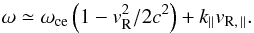 (3)For a given pair (ω, k∥), this condition defines a circle in the (v∥, v ⊥ ) plane. Radio wave amplification is achieved if the electron distribution function has dominant positive gradients (increase in the distribution function towards higher velocities) along this circle. Three typical distributions observed in the auroral regions have these characteristics: (i) the loss-cone resulting from collisions in the atmosphere of near-parallel downgoing electrons, which are always present; (ii) the horseshoe/shell distribution, resulting from acceleration parallel to the magnetic field (possibly steady state due to static electric fields); and (iii) a ring caused by acceleration parallel to the magnetic field at high latitudes (possibly impulsive, e.g. due to Alfvén waves). The most unstable mode for the CMI is, respectively (Hess et al. 2008a; Su et al. 2008):
-
(i)
 at
at  ;
; -
(ii)
 at k∥ = 0;
 -
(iii)
 at k∥ ~ vR, ∥ωce/(Nc2) ≥ 0,
where N is the refraction index that can be computed from the cold plasma dispersion relation, which takes different values at a given frequency and angle of propagation relative to the local magnetic field for left-hand ordinary (L-O) mode and right-hand extraordinary (R-X or R-Z) mode. Previous studies have shown that the R-Z mode cannot escape the plasma, CMI amplification is relatively inefficient for the L-O mode, and is efficient for the R-X mode if  is smaller than ~ 0.1 (Treumann 2006; Mottez et al. 2010). Since the R-X low frequency cutoff frequency is
  , shell emission below ωce meets a difficulty that can be overcome because in a hot plasma (several keV) the effective value of the cyclotron frequency in the electrons frame is ωce/γ < ωce, thus for low values of ωpe and large enough γ the R-X mode cutoff lies below ωce and emission is possible. In the Earth’s magnetosphere, interaction with the solar wind (so-called “Dungey-cycle” Dungey 1961), lead to the development of a steady state current circuit that leads to the formation of parallel electric fields and potential drops in the auroral regions. Those accelerate electrons (and ions) generating horseshoe/shell distributions, and at the same time carve density cavities in the auroral plasma, leading to the amplification of auroral radio waves in the shell mode (< ωce) (Roux et al. 1993).
In Jupiter’s magnetosphere, intense radio bursts are produced as a result of the interaction of Io with the rotating Jovian magnetic field. This interaction is short-lived for a given field line (duration < 1 min) and induces currents carried by Alfvén waves, which in turn accelerate electrons (Hess et al. 2007). Magnetic-field-aligned potential drops of up to 1 keV are also observed (Hess et al. 2009a,b). Simulation of these types of emission has shown that the loss-cone mode dominates if there is no plasma cavity, which is likely except near potential drops (Hess et al. 2008b). Radio emission is thus produced at oblique angles relative to the local magnetic field, resulting in a hollow conical beaming pattern (Mottez et al. 2010). This anisotropic beaming associated with the Jovian magnetic field topology causes the typical “arc” shape of Io-Jupiter decameter radio emissions in the time-frequency (t, f) plane, which was successfully modelled based on loss-cone driven CMI (Hess et al. 2008a, 2010a).
Finally, at Saturn, radio emission is due to the combination of the solar wind flow and the corotation of the magnetospheric plasma, driving Kelvin-Helmholtz waves and/or field-aligned currents (Galopeau et al. 1995). Radio emission is more intense on the morning side of the auroral regions, albeit present at all longitudes and local times (Lamy et al. 2008b). The emission morphology in the (t, f) plane mixes an unstructured continuum with drifting features and subcorotating arcs (Lamy et al. 2008a). The former might be linked to steady-state plasma acceleration up to a few keV by potential drops, while the latter might be related to Alfvénic acceleration up to 20 keV.
3. Numerical code
To simulate the intensity and polarization of the radio sources, we use the ExPRES numerical code that was originally designed to model the Io-Jupiter radio dynamic spectra (Hess et al. 2008a) and was later adapted to simulate any auroral radio source, such as those of Saturn (Lamy et al. 2008a), provided that the emission process is the CMI. The aim of this numerical code is to model the geometry of the emissions relative to the local magnetic field at various frequencies, to compute the direction of the emission at different locations based on the assumed energy source for the CMI, and to compare this direction to that of the observer relative to the source, to produce a modeled dynamic spectrum of the emission seen by the observer.
The first step is to define the location of the radio sources, via the longitude and latitude of the footprint(s) of the radio-emitting magnetic field line(s), and the frequency of the emission. By using a model of the magnetic field of the planet, the frequency of emissions, assumed to be the local cyclotron frequency of the electrons (fce), can be converted into the position of the source along the emitting magnetic field line(s).
The second step is to compute the direction of emission. The CMI amplifies waves that propagate along a hollow conical sheet whose axis is the local magnetic field vector. Refraction may occur in either the source or its immediate vicinity, as well as along the wave propagation between the source and the observer. The latter is generally neglected in planetary magnetospheres for the high frequency electron cyclotron waves considered here, and the former can be included in the description of the source’s beaming pattern. The parameters defining the direction of emission are hence the magnetic field vector – as provided by the magnetic field model – and the radio hollow cone aperture angle as a function of frequency (and possibly as a function of the azimuth around the magnetic field vector). This cone angle can be deduced from the CMI theory. For the most intense radio emission from Jupiter and Saturn, the radio hollow cone angle variation versus frequency can be well modelled by the directivity resulting from a loss-cone-driven instability, independent of the azimuth (Hess et al. 2008a; Ray & Hess 2008; Lamy et al. 2008a; Mottez et al. 2010), even when the actual source of free energy is not a loss-cone (Hess et al. 2008b, 2010b). We accordingly define the hollow cone aperture as  (4)where fmax is the electron cyclotron frequency at the footprint of the emitting magnetic field line (deduced from the magnetic field model) and v the velocity of the emitting electrons. By analogy with the typical energy of the electrons generating the auroral planetary radio emission in the Solar System (a few keV), this velocity is assumed to be v = 0.1 c in the present paper.
The last step is to compare the directions of emission with the direction of the observer – fixed or moving – as seen from each point of the source. A source point is visible if the two directions differ by an angle smaller than the hollow cone thickness, set to 1° in our simulation, consistent with the typical observed width of the hollow cones related to the Io-Jupiter emission (Queinnec & Zarka 1998; Kaiser et al. 2000).
The result of a run of ExPRES is a simulated dynamic spectrum similar to that that should be measured by the observer. In its simplest form, for a point source, each (t, f) element of this dynamic spectrum takes a value of one if emission is visible at the corresponding time and frequency, and zero when no emission is detected. For a distribution of point sources (corresponding to an extended source), the number of point sources visible at any given (t, f) approximates the received intensity. We also compute the dynamic spectrum of the observed polarization. For dominant X-mode emission (Zarka 1998), radio emission with 100% right-handed circular polarization is received from a northern magnetic hemisphere (of the star or of the planet), while 100% left-handed circular polarization is received from a southern magnetic hemisphere.
4. Simulation results
We simulate two models of interaction leading to the generation of radio emission, as described in the introduction: the first one assumes an Io-Jupiter-like interaction between the planet and its parent star, generating exoplanetary-induced stellar emission; the second one assumes a more usual stellar-wind driven interaction, generating exoplanetary magnetospheric emission. For each model, we considered an axisymmetric dipolar magnetic field of the emitting body, and a dipolar magnetic field tilted by 15° relative to the rotation axis of the emitting body. In each case, the simulations were performed assuming an inclination of the planetary orbital plane, relative to the observer’s line-of-sight, of 0°, 15°, 30°, 45°, 60°, 75°, and 90°. The inclinations correspond to an observer located northward of the orbiting plane. For southward inclinations, the same dynamic spectrum in intensity is obtained, but with inverted polarizations.
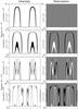 |
Fig. 1 Model dynamic spectra for an exoplanet-induced stellar emission. Abscissa is given in exoplanet’s years (i.e. orbital phase of the exoplanet) and stellar rotation (“* Rot”). In polarization dynamic spectra, black stands for northern emissions, white for southern emissions. a), b) Intensity and polarization dynamic spectra for an axisymmetric stellar magnetic field and 0° inclination (i.e. observer along the orbital plane). c), d) Intensity and polarization dynamic spectra for an axisymmetric stellar magnetic field and 15° inclination (i.e. observer’s direction 15° north of the orbital plane). e), f) Intensity and polarization dynamic spectra for a stellar magnetic field tilted by 15° relative to the rotation axis (perpendicular to the orbital plane) and 0° inclination. g), h) Intensity and polarization dynamic spectra for a stellar magnetic field tilted by 15° and 15° inclination. |
Regardless of either the interaction model or the magnetic field tilt, our simulations showed that almost no emission is visible for an inclination of the planetary orbital plane ≥ 60°. This kind of extinction was observed at Saturn by the Cassini spacecraft when the spacecraft latitude was larger than 45° (Lamy et al. 2008b). Consequently, only results obtained for lower inclinations are discussed here. This expected absence of visible emission for high orbit inclinations relative to the observer’s line-of-sight should have little consequence for radio detection because the main detection methods (i.e. transit and radial velocity) are biased towards the detection of exoplanets whose orbital plane has a low inclination relative to the observer’s line-of-sight.
4.1. Exoplanet-induced stellar emissions
The first model of interaction assumes an Io-Jupiter like interaction: the motion of the exoplanet relative to the corotating (or sub-corotating) stellar magnetic field generates a current along the field lines, utimately causing radio emission above the star’s surface. The high frequency cutoff of this emission is the electron cyclotron frequency at the star’s surface, whereas the low frequency cutoff corresponds to the distance at which the ratio of the plasma to cyclotron frequency (fpe/fce) becomes large enough (typically ≥ 0.3) to quench wave amplification by the CMI. In our simulations, the stellar magnetic field was assumed to be intense enough for the low frequency cutoff not to be observed. The radiosource region is modeled by point sources spread along an unique magnetic field line connecting the star to the exoplanet.
The plots in Fig. 1 show the intensity and polarization dynamic spectra obtained from this interaction model, for both axisymmetric and tilted stellar magnetic fields, and for inclinations of 0° and 15° of the exoplanet’s orbital plane relative to the observer’s line-of-sight.
All panels of Fig. 1 show radio arcs periodically occurring at a period equal to the orbital period of the planet, as expected for a single field line in corotation with the exoplanet. The same kind of dynamic spectrum is observed for the Io-Jupiter emission. The thickness of the arcs reflects the longitudinal extent of the emission region (in this simulation ~ 0) and the hollow cone thickness. For the tilted stellar magnetic field case, this occurrence period is modulated by the rotation period of the star, as the observer alternatively sees its northern and southern magnetic poles.
For an inclination of 0° and an axisymmetric magnetic field, the intensity and polarization dynamic spectra (panels a) and b)) show that both the northern and southern emissions together reach a maximum frequency that is close to the electron cyclotron frequency at the surface of the star. When the inclination increases (the observer lying increasingly northward of the orbital plane), the southern sources of emission reach lower maximum frequencies (panels c) and d)). This effect is also seen for the tilted stellar magnetic field case panels e) to h)).
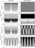 |
Fig. 2 Model dynamic spectra for the emission of the full auroral oval of an exoplanetary magnetosphere. Abscissa is given in exoplanet’s years (i.e. orbital phase of the exoplanet) and exoplanet’s days (i.e. rotational phase of the exoplanet). In polarization dynamic spectra, black stands for northern emissions, white for southern emissions. a), b) Intensity and polarization dynamic spectra for an axisymmetric planetary magnetic field and 0° inclination (i.e. observer along the orbital plane). c), d) Intensity and polarization dynamic spectra for an axisymmetric planetary magnetic field and 15° inclination (i.e. observer’s direction 15° north of the orbital plane). e), f) Intensity and polarization dynamic spectra for a planetary magnetic field tilted by 15° relative to the rotation axis (perpendicular to the orbital plane) and 0° inclination. g), h) Intensity and polarization dynamic spectra for a planetary magnetic field tilted by 15° and 15° inclination. |
4.2. Exoplanet magnetospheric emissions
The second model of interaction assumes that the star-exoplanet interaction results in auroral activity at the planet. Three sub-models of this induced auroral activity are considered here: a full auroral oval, active (emitting) at all latitudes, an active sector fixed in exoplanet’s longitude, and an active sector fixed in local time. All these scenarii have in common emission with a high frequency cutoff corresponding to the electron cyclotron frequency at the surface of the exoplanet. The low frequency cutoff occurs for a large plasma-to-cyclotron frequency ratio (fpe/fce), either in the source or along the wave trajectory, where the frequency of the emission drops below the local R-X mode cutoff. In our study, we assume that the exoplanet’s magnetic field is strong enough for the cutoff not to occur at the source. Outside the magnetosphere, however, the wave passes through the interplanetary medium, which is an extension of the stellar corona. Assuming a Solar-like parent star, i.e. relatively weakly magnetized, the R-X cutoff frequency can be assumed to be equal to the local plasma frequency, which is given by  (5)where the stellar wind number density N decreases with the distance to the star (d) as N ∝ d-2. The density at the stellar surface boundary is set to 2 × 106 cm-3, which results in stellar wind densities similar to the solar wind. The observed low-frequency cutoff is the consequence of the frequency-dependent apparent size of both the star (including the stellar corona and wind) and the planet (Fig. 5). Owing to the geometry of observation, the distance of closest approach (or impact parameter) of the radio waves relative to the star varies with the exoplanet’s orbital phase, so the observed low-frequency cutoff frequency varies accordingly. This effect is described in Sect. 6.3.
4.2.1. Full auroral oval
We modeled a full auroral oval by assuming that the sources are spread along 360 magnetic-field lines separated from each other by 1° in longitude. The active magnetic-field lines map to a circle with a radius of 20 exoplanetary radii at the equator, i.e, they form a magnetic shell of parameter L = 20. The active magnetic-field line footprints are thus at a latitude of ~ 77°.
The plots in Fig. 2 show the intensity and polarization dynamic spectra obtained from this interaction model, for both axisymmetric and tilted planetary magnetic fields, and for inclinations of 0° and 15° of the exoplanet’s orbital plane relative to the observer’s line-of-sight.
For an inclination of 0° and an axisymmetric magnetic field, no modulation of the intensity of the source is observed, except the one caused by the shielding of the emission by the star, stellar corona, and interplanetary medium, i.e. the modulation of the low-frequency cutoff at the exoplanet’s orbital period. The amplitude of modulation of this cutoff decreases for increasing inclinations, as discussed in Sect. 6.3.
As for the exoplanet-induced stellar emission, the intensity and polarization dynamic spectra (panels a) and b)) show that at 0° inclination, both the northern and southern emissions reach together a maximum frequency close to the electron cyclotron frequency at the surface of the planet. When the inclination increases (the observer lying increasingly northward of the orbital plane) the southern hemisphere emissions reach lower maximum frequencies. The same effect is also produced by the tilted magnetic field.
For such a tilted magnetic field, the intensity dynamic spectrum shows a modulation at the exoplanetry rotation period caused by the observer seeing alternatively the northern and southern magnetic poles.
4.2.2. Active sector fixed in longitude
We modeled an active sector of width arbitrarily chosen to be equal to 12° by assuming emission sources spread along 13 active magnetic field lines separated from each other by 1° in longitude. As in the full auroral oval case, the active magnetic field lines cross the equatorial plane of the planet at a distance of 20 exoplanetary radii from the planet.
The plots in Fig. 3 show the intensity and polarization dynamic spectra obtained from this interaction model, for both axisymmetric and tilted planetary magnetic fields and for inclinations of 0° and 15°.
The properties of the emissions are close to those of the full oval, except that the emission appears as discrete arcs rather than a continuum, with a recurrence period equal to the exoplanetary rotation period. This is obviously due to the variation in the source phase relative to the observer’s direction, caused by the exoplanetary rotation. The width of the arcs is the sum of the longitudinal interaction region size and the hollow cone thickness.
In constrast to the previous models of interaction, the northern and southern arcs appear to be in phase even for a tilted magnetic field because even if the observer sees alternatively the two magnetic poles, the emissions only occur within a given longitude range, considered here to be the same in both hemispheres. This leads to an apparent inability to differenciate between the dynamic spectrum obtained for an axisymmetric field observed with an inclination of 15° and a magnetic field tilted by 15° observed with an inclination of 0°. The only way to discriminate between these cases is the variation in the low frequency cutoff due to the stellar wind/interplanetary plasma, which is related to the inclination only and is thus different for an observation with an inclination of 15° and 0°.
4.2.3. Active sector fixed in local time
We again modeled a 12° wide active sector by assuming that the emission sources are spread along 13 active magnetic field lines separated from each other by 1° in longitude. The active magnetic field lines again map to a distance of 20 exoplanetary radii at the equator. However, the longitudes of the active magnetic field lines vary with the exoplanetary rotation such that the local times of the sources remain constant, i.e., their position remains constant relative to the direction of the central star (at 12h local time).
The plots in Fig. 4 show the intensity and polarization dynamic spectra obtained from this interaction model, for both axisymmetric and tilted planetary magnetic fields and for inclinations of 0° and 15°.
Apart from the low frequency cutoff produced by the shielding of the emission by the weakly magnetized stellar wind, our simulation results are comparable to those obtained for exoplanet-induced stellar emission (Sect. 4.1): the sources fixed in local time are also fixed in the star-centered reference frame in corotation with the planet at its orbital speed. For an axisymmetric magnetic-field, the low frequency cutoff is the major difference between this auroral case and the stellar emission case. The other difference between these types of emission is their phase shift, when we assume the orbital phase of the planet as a reference, shift that depends on the position of the active sector in local time. For example, if the active sector were centered on midnight, the emissions would be in phase, while they would be in antiphase for an active sector centered at noon.
For a tilted magnetic field, there is another difference: the alternation between the two polarizations occurs in accordance with the planetary rotation period instead of the stellar rotation period (the former here being longer than the latter).
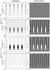 |
Fig. 3 Model dynamic spectra for the emission of an active sector fixed in longitude along the auroral oval of an exoplanetary magnetosphere. Abscissa is similar to Fig. 2. In polarization dynamic spectra, black stands for northern emissions, white for southern emissions. a), b) Intensity and polarization dynamic spectra for an axisymmetric planetary magnetic field and 0° inclination. c), d) Intensity and polarization dynamic spectra for an axisymmetric planetary magnetic field and 15° inclination. e), f) Intensity and polarization dynamic spectra for a planetary magnetic field tilted by 15° relative to the rotation axis and 0° inclination. g), h) Intensity and polarization dynamic spectra for a planetary magnetic field tilted by 15° and 15° inclination. |
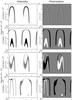 |
Fig. 4 Model dynamic spectra for the emission of an active sector of the auroral oval of an exoplanetary magnetosphere fixed in local time. Abscissa is similar to Fig. 2. In polarization dynamic spectra, black stands for northern emissions, white for southern emissions. a), b) Intensity and polarization dynamic spectra for an axisymmetric planetary magnetic field and 0° inclination. c), d) Intensity and polarization dynamic spectra for an axisymmetric planetary magnetic field and 15° inclination. e), f) Intensity and polarization dynamic spectra for a planetary magnetic field tilted by 15° relative to the rotation axis and 0° inclination. g), h) Intensity and polarization dynamic spectra for a planetary magnetic field tilted by 15° and 15° inclination. |
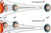 |
Fig. 5 Sketch of the variation in the low frequency cutoff with the phase φ and the inclination i. The apparent sizes of the star (including its stellar wind) and the planet increase as the observed frequency decreases. Hence, the closer to the star the planet appears in projection on the plane of the the sky, the higher is the cutoff frequency. The gray zones delimited by the continuous and dashed lines corresponds to the regions where the solar wind plasma frequencies are higher than two frequencies f1 and f2 < f1, respectively. The green and blue regions surrounding the exoplanet are the apparent diameter of the planet (emission region) at the frequencies f1 and f2. The upper panel shows the case of a 0° inclination. In this case, as the planet apparent position is closer to the star, the radio emission from the planet becomes shielded, at low frequency first. This shielding occurs at a slower rate for larger inclinations of the planet orbit (lower panel). Note that this sketch is not to scale, the size of the star being much larger than that of the planet. |
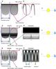 |
Fig. 6 Summary sketch illustrating how physical parameters of the system are related to specific features of the observed dynamic spectra. a)–c) Planetary magnetic field tilted by 0° relative to the rotation axis and 0° inclination, for a) the full auroral oval interaction model and b) an auroral active sector fixed in local time. d)–f) Planetary magnetic field tilted by 0° and 15° inclination, for the full auroral oval interaction model. g)–i) Planetary magnetic field tilted by 15° and 0° inclination, for the full auroral oval interaction model. |
5. Discriminating between the interaction models
When radio emission from exoplanetary systems is eventually detected and their dynamic spectra measured with sufficient signal-to-noise ratio (SNR), the next challenge will be to draw physical information from the observations. The first step in interpreting the observed dynamic spectra, or in the present case the modelled ones, is to determine the interaction model to which it applies (Fig. 6).
If the emission is a continuum with only a modulation of the low frequency cutoff and a modulation of the wave polarization, the interaction model is the full auroral oval one. If the wave polarization is itself modulated, the exoplanet’s magnetic field is tilted by an angle that can be deduced from the shape of this modulation.
If the emission is a discrete arc recurring with the orbital period and there is no shielding of the low frequency part of the emission by the stellar wind, the interaction model is the exoplanet-induced stellar emission one. We note that a secondary modulation can be attributed to the stellar rotation period if the stellar magnetic field is tilted.
If the emission is an arc occurring with the orbital period and there is shielding of the low frequency part of the emissions by the stellar wind, the interaction model is that for which the active sector is fixed in local time. Here a secondary modulation can be attributed to the exoplanet’s rotation period if the exoplanetary magnetic field is tilted.
Finally, if the emission is an arc whose main occurrence period is not the orbital period the interaction model is that for which the active sector fixed in longitude. We note that the orbital period then appears as a secondary, superimposed modulation period.
6. Orbital parameter determination
6.1. Magnetic field strength
Our simulations show that the highest frequency reached by the radio emission is close to the electron cyclotron frequency at the surface of the emitting body. Since the electron cyclotron frequency is proportional to the magnetic field amplitude, the measurement of the maximum frequencies in the dynamic spectra enables us to infer the magnetic field amplitudes at or near the surface of the exoplanet (or of the star) along the footprints of the active field lines. The radio observation of an exoplanet is thus likely to be the most straightforward way to estimate the amplitude of the exoplanetary magnetic field.
6.2. Orbital period
For all interaction models, our simulation results show a modulation of the emission with the planetary orbital period. This modulation is often superimposed on a second one at the stellar or planetary rotation period. Since the orbital period is easily determined by most of the available exoplanet detection methods (radial velocities, transits, ...), we use these independent determinations to distinguish the observed modulations and infer the superimposed planetary or stellar rotation period (cf. Sect. 6.5). Radio observations can thus provide a measure of the exoplanet’s orbital period, but this determination is not the main motivation for radio observations.
6.3. Orbit inclination
From the results of our simulations, there are two main ways to deduce the inclination of the orbital plane of the exoplanet. The first is to compare the maximum frequencies of the emission from the two hemispheres (with opposite polarizations). The magnetic field tilt is not an issue because it only causes the emission from opposite hemispheres to be out-of-phase. The above maximum frequency in each polarization just needs to be determined over a long enough interval. However, for an active sector fixed in longitude, the observed maximum frequency in each hemisphere is the one at the footprints of active field lines in the corresponding longitude range only, thus it is then impossible to differentiate between a tilted magnetic field and an inclined orbit. Moreover if the center of the magnetic dipole is offset from the planet’s center – which has not been modelled in the present study – the ratio of maximum frequencies reached by northern to southern emissions does not only depends on the orbit inclination but also on the dipole offset. Thus, the maximum frequency ratio is not the most reliable way to measure the orbit inclination.
The second method for determining the inclination of the exoplanet’s orbital plane is to measure the low frequency cutoff of the emissions. This cutoff depends on both the phase of the exoplanet’s orbital motion, and on the inclination of its orbit (Fig. 5). For orbital phases − 90° ≤ φ ≤ 90° (i.e. when the exoplanet is on the anti-observer part of its orbit, the origin of orbital phases being taken at the anti-observer point as for the Io phase around Jupiter (Zarka et al. 1996)), the value of the low frequency cutoff corresponds to the highest plasma frequency (highest density) encountered by the wave along the line-of-sight. In the present paper, we assumed a spherically symmetric density model for the stellar wind and a radial dependence of the density N ∝ d-2 (where N is the electron density and d the radial distance from the star). The highest density thus corresponds to the distance of closest approach (or impact parameter) of the radio waves relative to the star. This distance d, which is also the apparent distance from the exoplanet to the star at phase φ, can be expressed as 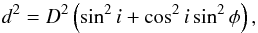 (6)where D is the exoplanet orbit radius and i the inclination as defined above. Taking into acount Eq. (5), the low frequency cutoff at phase fco(φ) can be expressed as a function of this cutoff when the exoplanet is at either limb of the star, i.e. fco(φ = ± 90°), as
 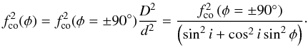 (7)The inclination can thus be deduced from the observed variation in the low frequency cutoff for exoplanet phases − 90° ≤ φ ≤ 90°
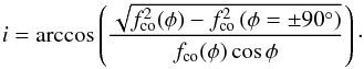 (8)This equation can be easily modified to take into account second order terms, such as a lack of spherical symmetry in the stellar wind density. This method provides the most accurate value of the inclination and should then be used whenever possible. For the exoplanet-induced stellar emission model, this method cannot be applied as the stellar wind shielding (neglected here) does not depend on the exoplanet’s phase, but rather the distance from the star at which the ratio of the plasma to cyclotron frequency (fpe/fce) becomes sufficiently large (typically ≥ 0.3) to prevent the CMI amplification of the waves inside the source.
6.4. Magnetic field tilt or offset
The case of a magnetic dipole with an offset has not been simulated in the present study, mainly because the number of possible magnetic field geometries is large so we had to select only few representative cases. The expected effect of a magnetic dipole offset is to cause a different value of the surface magnetic field in opposite hemispheres. This can lead to a confusion between the effect of a magnetic tilt offset and that of orbit inclination, so the orbit inclination must be computed first using the above low-frequency cutoff method whenever applicable (not for stellar emissions).
The effect of a magnetic field tilt is to put out-of-phase the emissions from the two opposite hemispheres, as the observer will see different magnetic hemispheres when he observes different active longitudes. It should be possible to distinguish between a magnetic dipole tilt and a magnetic dipole offset, as they produce different effects on the observed emissions. However, for an active sector fixed in longitude, this difference is not visible because the emission only occurs for a limited range of longitudes, i.e., the observer always faces the same magnetic hemisphere when the emissions occur.
6.5. Exoplanet rotation period and stellar rotation period
When exoplanet magnetospheric emission is caused by an active sector fixed in longitude, the rotation period of the exoplanet is the main periodic modulation of the observed (t, f) radio arcs. In all other models of exoplanetary magnetospheric auroral emission, the rotation period is the modulation due to the tilt of the exoplanetary magnetic field superimposed on the modulation at the exoplanet’s orbital period. For an exoplanet-induced stellar emission, the rotation period of the exoplanet remains unknown but the stellar rotation period is inferred from the modulations produced by the tilt of the stellar magnetic field superimposed on the modulation at the exoplanet’s orbital period.
7. Discussion
We have simulated the radio dynamic spectra resulting from the four typical interaction models between an exoplanet and its parent star leading to the generation of radio emission by means of the CMI mechanism. This will enable us to derive physical information from the first detections of radio emissions from exoplanetary systems, which we expect to be achieved by the extensive programs running or about to start using large radiotelescopes such as LOFAR, UTR2, or the GMRT. These observations will be in the form of dynamic spectra, as star-exoplanet systems will also be unresolved in radio, especially hot Jupiter systems. The simulations discussed in the present paper cover neither all possible cases of interaction nor all possible physical parameters of the studied systems, but provide the basic methodology that can easily be adapted to specific observations, once effective detection has been achieved. In particular, more complex stellar or exoplanetary magnetic field models can be considered, as well as non-spherical stellar wind models, elliptical planetary orbits, etc.
Figure 6 illustrates in a synthetic way how physical parameters can be drawn from specific parts of the observed dynamic spectra. Panels a)–c) correspond to an orbit inclination and a magnetic tilt that are both equal to 0°, and they show that the type of interaction will be deduced from the general (t, f) shape of the emission (e.g. continuum for a full oval (a) or arcs for an active sector fixed in local time (b)), the magnetic moment of the emitting body will be given by the maximum frequency of the emission, and the orbital period by its main modulation. Panels d)–f), corresponding to the the full oval case with a magnetic tilt of 0° and an orbit inclination of 15°, show in addition that the orbit inclination can be inferred from the polarization pattern and by the shape of the low frequency cutoff of the emission. Finally, panels g)–i), corresponding to the the full oval case with an orbit inclination of 0° and a magnetic tilt of 15°, show how the rotation period and dipole tilt of the exoplanet are revealed by the secondary modulation of the intensity and polarization patterns and their detailed shape.
Dynamic spectra discussed here are noiseless. However, as mentioned in Sect. 1, initial observations with typical integration
over ~1 MHz × 1 min dynamic spectral bins will have a low SNR. Observation and data analysis strategies can be developed to increase the SNR of dynamic spectra, which would involve longer integration time bins (≥ 10 min), detection of periodicities in the signal integrated over its full bandwidth (up to tens of MHz) followed by time folding and integration of dynamic spectra at each of the detected periods (orbital, planetary rotation, stellar rotation). Finally, we again note that the methodology developed in this paper is fully applicable to the case of radio emission produced by magnetic white dwarf-planet or white dwarf-brown dwarf systems (Willes & Wu 2004, 2005, and references therein).
References
- Dungey, J. W. 1961, Phys. Rev. Lett., 6, 47 [NASA ADS] [CrossRef] [Google Scholar]
- Ellingson, S. W., Clarke, T. E., Cohen, A., et al. 2009, IEEE Proc., 97, 1421 [Google Scholar]
- Farrell, W. M., Desch, M. D., & Zarka, P. 1999, J. Geophys. Res. (Space Phys.), 104, 14025 [NASA ADS] [CrossRef] [Google Scholar]
- Fender, R. P., Wijers, R. A. M. J., Stappers, B., et al. 2006, in VI Microquasar Workshop: Microquasars and Beyond [Google Scholar]
- Galopeau, P. H. M., Zarka, P., & Quéau, D. L. 1995, J. Geophys. Res., 100, 26397 [Google Scholar]
- Grießmeier, J., Zarka, P., & Spreeuw, H. 2007, A&A, 475, 359 [NASA ADS] [CrossRef] [EDP Sciences] [Google Scholar]
- Hess, S., Mottez, F., & Zarka, P. 2007, J. Geophys. Res., 112, A11212 [NASA ADS] [CrossRef] [Google Scholar]
- Hess, S., Cecconi, B., & Zarka, P. 2008a, Geophys. Res. Lett., 35, 13107 [NASA ADS] [CrossRef] [Google Scholar]
- Hess, S., Mottez, F., & Zarka, P. 2008b, J. Geophys. Res., 113, A03209 [NASA ADS] [Google Scholar]
- Hess, S., Mottez, F., & Zarka, P. 2009a, Geophys. Res. Lett., 36, 14101 [NASA ADS] [CrossRef] [Google Scholar]
- Hess, S., Zarka, P., Mottez, F., & Ryabov, V. B. 2009b, Planet. Space Sci., 57, 23 [NASA ADS] [CrossRef] [Google Scholar]
- Hess, S., Petin, A., Zarka, P., Bonfond, B., & Cecconi, B. 2010a, Planet. Space Sci., 58, 1188 [NASA ADS] [CrossRef] [Google Scholar]
- Hess, S. L. G., Delamere, P., Dols, V., Bonfond, B., & Swift, D. 2010b, J. Geophys. Res. (Space Phys.), 115, 6205 [Google Scholar]
- Kaiser, M. L., Zarka, P., Kurth, W. S., Hospodarsky, G. B., & Gurnett, D. A. 2000, J. Geophys. Res., 105, 16053 [NASA ADS] [CrossRef] [MathSciNet] [Google Scholar]
- Lamy, L., Zarka, P., Cecconi, B., Hess, S., & Prangé, R. 2008a, J. Geophys. Res. (Space Phys.), 113, 10213 [Google Scholar]
- Lamy, L., Zarka, P., Cecconi, B., et al. 2008b, J. Geophys. Res. (Space Phys.), 113, 7201 [Google Scholar]
- Lazio, T. J. W., & Farrell, W. M. 2007, ApJ, 668, 1182 [NASA ADS] [CrossRef] [Google Scholar]
- Lecavelier Des Etangs, A., Sirothia, S. K., Gopal-Krishna, & Zarka, P. 2009, A&A, 500, L51 [NASA ADS] [CrossRef] [EDP Sciences] [Google Scholar]
- McIlwain, C. E. 1961, J. Geophys. Res., 66, 3681 [Google Scholar]
- Mottez, F., Hess, S., & Zarka, P. 2010, Planet. Space Sci., 58, 1414 [NASA ADS] [CrossRef] [Google Scholar]
- Nichols, J. D. 2011, MNRAS, in press [Google Scholar]
- Queinnec, J., & Zarka, P. 1998, J. Geophys. Res., 103, 26649 [NASA ADS] [CrossRef] [Google Scholar]
- Ray, L. C., & Hess, S. 2008, J. Geophys. Res., 113, A11218 [NASA ADS] [Google Scholar]
- Roux, A., Hilgers, A., de Feraudy, H., et al. 1993, J. Geophys. Res., 98, 11657 [NASA ADS] [CrossRef] [Google Scholar]
- Ryabov, V. B., Zarka, P., & Ryabov, B. P. 2004, Planet. Space Sci., 52, 1479 [NASA ADS] [CrossRef] [Google Scholar]
- Sánchez-Lavega, A. 2004, ApJ, 609, L87 [NASA ADS] [CrossRef] [Google Scholar]
- Su, Y.-J., Ma, L., Ergun, R. E., Pritchett, P. L., & Carlson, C. W. 2008, J. Geophys. Res. (Space Phys.), 113, 8214 [NASA ADS] [CrossRef] [Google Scholar]
- Treumann, R. A. 2006, A&AR, 13, 229 [CrossRef] [Google Scholar]
- Willes, A. J., & Wu, K. 2004, MNRAS, 348, 285 [NASA ADS] [CrossRef] [Google Scholar]
- Willes, A. J., & Wu, K. 2005, A&A, 432, 1091 [NASA ADS] [CrossRef] [EDP Sciences] [Google Scholar]
- Wu, C. S. 1985, Space Sci. Rev., 41, 215 [NASA ADS] [CrossRef] [Google Scholar]
- Zarka, P. 1998, J. Geophys. Res., 103, 20159 [NASA ADS] [CrossRef] [Google Scholar]
- Zarka, P. 2000, in Radio Astronomy at Long Wavelengths, ed. R. G. Stone, K. W. Weiler, M. L. Goldstein, & J.-L. Bougeret, 167 [Google Scholar]
- Zarka, P. 2004a, in Extrasolar Planets: Today and Tomorrow, ed. J. Beaulieu, A. Lecavelier Des Etangs, & C. Terquem, ASP Conf. Ser., 321, 160 [Google Scholar]
- Zarka, P. 2004b, Adv. Space Res., 33, 2045 [NASA ADS] [CrossRef] [Google Scholar]
- Zarka, P. 2007, Planet. Space Sci., 55, 598 [NASA ADS] [CrossRef] [Google Scholar]
- Zarka, P. 2010, in EAS Pub. Ser. 41, ed. T. Montmerle, D. Ehrenreich, & A.-M. Lagrange, 441 [Google Scholar]
- Zarka, P., Farges, T., Ryabov, B. P., Abada-Simon, M., & Denis, L. 1996, Geophys. Res. Lett., 23, 125 [NASA ADS] [CrossRef] [Google Scholar]
- Zarka, P., Treumann, R. A., Ryabov, B. P., & Ryabov, V. B. 2001, Ap&SS, 277, 293 [Google Scholar]
All Figures
|
Fig. 1 Model dynamic spectra for an exoplanet-induced stellar emission. Abscissa is given in exoplanet’s years (i.e. orbital phase of the exoplanet) and stellar rotation (“* Rot”). In polarization dynamic spectra, black stands for northern emissions, white for southern emissions. a), b) Intensity and polarization dynamic spectra for an axisymmetric stellar magnetic field and 0° inclination (i.e. observer along the orbital plane). c), d) Intensity and polarization dynamic spectra for an axisymmetric stellar magnetic field and 15° inclination (i.e. observer’s direction 15° north of the orbital plane). e), f) Intensity and polarization dynamic spectra for a stellar magnetic field tilted by 15° relative to the rotation axis (perpendicular to the orbital plane) and 0° inclination. g), h) Intensity and polarization dynamic spectra for a stellar magnetic field tilted by 15° and 15° inclination. |
| In the text | |
|
Fig. 2 Model dynamic spectra for the emission of the full auroral oval of an exoplanetary magnetosphere. Abscissa is given in exoplanet’s years (i.e. orbital phase of the exoplanet) and exoplanet’s days (i.e. rotational phase of the exoplanet). In polarization dynamic spectra, black stands for northern emissions, white for southern emissions. a), b) Intensity and polarization dynamic spectra for an axisymmetric planetary magnetic field and 0° inclination (i.e. observer along the orbital plane). c), d) Intensity and polarization dynamic spectra for an axisymmetric planetary magnetic field and 15° inclination (i.e. observer’s direction 15° north of the orbital plane). e), f) Intensity and polarization dynamic spectra for a planetary magnetic field tilted by 15° relative to the rotation axis (perpendicular to the orbital plane) and 0° inclination. g), h) Intensity and polarization dynamic spectra for a planetary magnetic field tilted by 15° and 15° inclination. |
| In the text | |
|
Fig. 3 Model dynamic spectra for the emission of an active sector fixed in longitude along the auroral oval of an exoplanetary magnetosphere. Abscissa is similar to Fig. 2. In polarization dynamic spectra, black stands for northern emissions, white for southern emissions. a), b) Intensity and polarization dynamic spectra for an axisymmetric planetary magnetic field and 0° inclination. c), d) Intensity and polarization dynamic spectra for an axisymmetric planetary magnetic field and 15° inclination. e), f) Intensity and polarization dynamic spectra for a planetary magnetic field tilted by 15° relative to the rotation axis and 0° inclination. g), h) Intensity and polarization dynamic spectra for a planetary magnetic field tilted by 15° and 15° inclination. |
| In the text | |
|
Fig. 4 Model dynamic spectra for the emission of an active sector of the auroral oval of an exoplanetary magnetosphere fixed in local time. Abscissa is similar to Fig. 2. In polarization dynamic spectra, black stands for northern emissions, white for southern emissions. a), b) Intensity and polarization dynamic spectra for an axisymmetric planetary magnetic field and 0° inclination. c), d) Intensity and polarization dynamic spectra for an axisymmetric planetary magnetic field and 15° inclination. e), f) Intensity and polarization dynamic spectra for a planetary magnetic field tilted by 15° relative to the rotation axis and 0° inclination. g), h) Intensity and polarization dynamic spectra for a planetary magnetic field tilted by 15° and 15° inclination. |
| In the text | |
|
Fig. 5 Sketch of the variation in the low frequency cutoff with the phase φ and the inclination i. The apparent sizes of the star (including its stellar wind) and the planet increase as the observed frequency decreases. Hence, the closer to the star the planet appears in projection on the plane of the the sky, the higher is the cutoff frequency. The gray zones delimited by the continuous and dashed lines corresponds to the regions where the solar wind plasma frequencies are higher than two frequencies f1 and f2 < f1, respectively. The green and blue regions surrounding the exoplanet are the apparent diameter of the planet (emission region) at the frequencies f1 and f2. The upper panel shows the case of a 0° inclination. In this case, as the planet apparent position is closer to the star, the radio emission from the planet becomes shielded, at low frequency first. This shielding occurs at a slower rate for larger inclinations of the planet orbit (lower panel). Note that this sketch is not to scale, the size of the star being much larger than that of the planet. |
| In the text | |
|
Fig. 6 Summary sketch illustrating how physical parameters of the system are related to specific features of the observed dynamic spectra. a)–c) Planetary magnetic field tilted by 0° relative to the rotation axis and 0° inclination, for a) the full auroral oval interaction model and b) an auroral active sector fixed in local time. d)–f) Planetary magnetic field tilted by 0° and 15° inclination, for the full auroral oval interaction model. g)–i) Planetary magnetic field tilted by 15° and 0° inclination, for the full auroral oval interaction model. |
| In the text | |
Current usage metrics show cumulative count of Article Views (full-text article views including HTML views, PDF and ePub downloads, according to the available data) and Abstracts Views on Vision4Press platform.
Data correspond to usage on the plateform after 2015. The current usage metrics is available 48-96 hours after online publication and is updated daily on week days.
Initial download of the metrics may take a while.