| Issue |
A&A
Volume 531, July 2011
|
|
|---|---|---|
| Article Number | A156 | |
| Number of page(s) | 15 | |
| Section | Astronomical instrumentation | |
| DOI | https://doi.org/10.1051/0004-6361/201016419 | |
| Published online | 05 July 2011 | |
Kernel spectral clustering of time series in the CoRoT exoplanet database
1
Department of Electrical Engineering ESAT-SCD-SISTAKatholieke Universiteit Leuven, Kasteelpark Arenberg 10, 3001 Leuven, Belgium
e-mail: This email address is being protected from spambots. You need JavaScript enabled to view it.
; This email address is being protected from spambots. You need JavaScript enabled to view it.
; This email address is being protected from spambots. You need JavaScript enabled to view it.
;
2
Instituut voor Sterrenkunde, Katholieke Universiteit Leuven, Celestijnenlaan 200D, 3001 Leuven, Belgium
e-mail: This email address is being protected from spambots. You need JavaScript enabled to view it.
Received: 29 December 2010
Accepted: 27 April 2011
Abstract
Context. Detection of contaminated light curves and irregular variables has become a challenge when studying variable stars in large photometric surveys such as that produced by the CoRoT mission.
Aims. Our goal is to characterize and cluster the light curves of the first four runs of CoRoT, in order to find the stars that cannot be classified because of either contamination or exceptional or non-periodic behavior.
Methods. We study three different approaches to characterize the light curves, namely Fourier parameters, autocorrelation functions (ACF), and hidden Markov models (HMMs). Once the light curves have been transformed into a different input space, they are clustered, using kernel spectral clustering. This is an unsupervised technique based on weighted kernel principal component analysis (PCA) and least squares support vector machine (LS-SVM) formulations. The results are evaluated using the silhouette value.
Results. The most accurate characterization of the light curves is obtained by means of HMM. This approach leads to the identification of highly contaminated light curves. After kernel spectral clustering has been implemented onto this new characterization, it is possible to separate the highly contaminated light curves from the rest of the variables. We improve the classification of binary systems and identify some clusters that contain irregular variables. A comparison with supervised classification methods is also presented.
Key words: stars: variables: general / binaries: general / techniques: photometric / methods: data analysis / methods: statistical
© ESO, 2011
1. Introduction
An enormous volume of astrophysical data has been collected in the past few years by means of ground and space-based telescopes. This is mainly due to an incredible improvement in the sensitivity and accuracy of the instruments used for observing and detecting phenomena such as stellar oscillations and planetary transits. Oscillations provide very important insight into the internal structure of the stars, and can be studied from the light curves (or time series). These are a collection of data points that result from measuring the brightness of the stars at different moments in time. An example of a space-based mission is the COnvection, ROtation & planetary Transits (CoRoT) satellite (Fridlund et al. 2006; Auvergne et al. 2009). The main goals of CoRoT are to detect planets outside our solar system and study stellar variability. Another important example is the ongoing Kepler mission (Borucki et al. 2010). This satellite is exploring the structure and diversity of extrasolar planetary systems, and measures the stellar variability of the host stars. More than 100 000 light curves will be collected by this satellite. Our ambitions are of course not limited to these projects. The GAIA satellite will observe the sky as no instrument has ever done before. Its main goal is to create the most precise three-dimensional map of the Milky Way. This mission will extend our knowledge on, amongst others, the field of stellar evolution, by observing more than one billion stars!
Missions like these play an important role in the development of our astrophysical understanding. But how does one extract useful information from this abundance of data? To start with, one can group the time series into sets with similar properties and generate a catalogue. This allows for easier selection of particular objects, leaving more time for fundamental astronomical research.
There exist two ways of learning the underlying structure of a dataset, namely supervised and unsupervised methods. In the supervised approach, it is necessary to predefine the different variability classes expected to be present in the dataset. For the unsupervised techniques on the other hand, the dataset is divided into natural substructures (clusters), without the need to specify any prior information. The main advantage of clustering (Jain et al. 1999) over supervised classification is the possibility of discovering new clusters that can be associated with new variability types.
In astronomy, some computational classification methods have already been implemented and applied to different datasets. The most popular automated clustering technique is the Bayesian parametric modeling methodology, AUTOCLASS, proposed by Cheeseman et al. (1988) and used by Eyer & Blake (2005) to study the ASAS variable stars. Hojnacki et al. (2008) applied unsupervised classification algorithms in the Chandra X-ray Observatory to classify X-ray sources. Debosscher (2009) applied supervised classification techniques to the OGLE and CoRoT databases. Sarro et al. (2009) reported on the results of clustering variable stars in the Hipparcos, OGLE, and CoRoT databases, using probability density distributions in attribute space. Some of the Kepler Q1 long-cadence light curves were previously classified in Blomme et al. (2010), where multi-stage trees and Gaussian mixtures were used to classify a sub-sample of 2288 stars.
Until now, the supervised classification and clustering techniques applied to the CoRoT dataset, have been based on a multidimensional attribute space, which consists of three frequencies and four harmonics at each frequency, that are extracted from the time series using Fourier analysis. The methodology to extract these attributes is described in Debosscher et al. (2007) and has some disadvantages that can be seen as follows. We consider a monoperiodic and a multiperiodic variable. The first one can be described by a single frequency and amplitude, while the second consists of a combination of different frequencies, amplitudes and phases. By forcing the set of parameters to be equal for all the stars, including the irregular ones, it is likely to end up with incomplete characterization for some of the light curves. This can later be related to misclassifications. There are other limitations to the techniques that are so far used to analyse the CoRoT dataset. For the supervised techniques, it is not possible to find new variability classes. However, unsupervised algorithms such as k-means and hierarchical clustering assume an underlying distribution of the data. This is undesirable when the attribute space becomes more complex. To solve this problem, we propose to use another unsupervised learning technique, namely spectral clustering.
The CoRoT dataset is highly contaminated by instrumental systematics. The orbital period, long-term trends, and spurious frequencies are some of the impurities present in the data. Options to correct for these instrumental effects are discussed in Debosscher (2009). Discontinuities in the light curves are also present. This is a consequence of contaminants such as cosmic rays hitting the CCD. New methods to clean the light curves have therefore been developed. The majority of these techniques give significant improvements when applied to individual light curves, but in cases where systematics of big datasets need to be removed, these techniques are inefficient. All these contaminants can be confused with real oscillation frequencies. For example, jumps in the light curves can be interpreted as eclipses or vice versa. Figure 1 shows the two candidate eclipsing binaries resulting after applying supervised (Debosscher et al. 2009) and k-means to the fixed set of Fourier attributes. If one wishes to clean the dataset of either systematics or jumps without affecting the signal of eclipsing binaries, it is necessary to separate the binary systems in some way, or detect the contaminated light curves. This can be achieved by performing a new characterization of the light curves and applying different classification or clustering techniques.
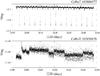 |
Fig. 1 Two eclipsing binaries (ECL) candidates obtained by supervised classification (Debosscher et al. 2009) and k-means on the fixed set of Fourier attributes. Top: real candidate ECL. Bottom: contaminated light curve. |
This work presents the application of kernel spectral clustering to different characterizations of the CoRoT light curves. Three different ways of modeling the light curves are presented in Sect. 2. In Sect. 3, we describe the spectral clustering algorithm used to cluster the light curves, which was proposed in Alzate & Suykens (2010). Section 4 is devoted to the clustering results of the three different characterizations of light curves. We compare our partition with the previous supervised classification results presented in Debosscher et al. (2009). Finally, in Sect. 5 we present the conclusions of our work and some future directions of this research.
2. Time series analysis
The light curves (time series) analysed in this work belong to the first four observing runs of CoRoT: IRa01, LRa01, LRc01, and SRc01. The stars were observed during different periods of time, producing time series of unequal length. In addition the sampling time is 32 s, but for the majority of the stars an average over 16 samples was taken. This results in an effective sampling time of 512 s. Consequently, the dataset contains a time series with different sampling times. To facilitate the analysis, we re-sample all the light curves with a uniform sampling time equal to 512 s. Owing the high resolution of the light curves, it is possible to use interpolation, without affecting the spectrum. This was tested in Degroote et al. (2009b) and is repeated in this work.
Three different characterizations are evaluated. We first propose to use the autocorrelation functions (ACFs) of the time series as a new characterization of the light curves. Second, a modification of the attribute extraction proposed in Debosscher et al. (2007) is implemented. Finally, each time series is modeled by a hidden Markov model (HMM). This leads to a new set of parameters that can be used to cluster the stars. The idea behind this is to find out how likely it is that a certain time series is generated by a given HMM. This was proposed in Jebara & Kondor (2003) and a variation of this method, together with its application to astronomical dataset is proposed here.
2.1. Autocorrelation functions
The autocorrelation of the power spectrum is an important tool for studing the stellar interiors, because it provides information about the small frequency separation between different oscillation modes inside the stars (Aerts et al. 2010). From these separations it is possible to infer information such as the mass and evolutionary state of the star. In other words, the small frequency separation is an indicator of the evolutionary state of the star that is directly associated with its variability class.
In Roxburgh & Vorontsov (2006), the determination of the small separation from the ACF of the time series is described. This is useful, especially in this application, where highly contaminated spectra are expected because of systematics and other external effects. Furthermore, the identification of single oscillation frequencies is unreliable. Taking into account the information that can be obtained from the ACF, we proposed to use it to differentiate between the different variability classes.
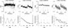 |
Fig. 2 Autocorrelation function of four CoRoT light curves. Top: original light curves. Bottom: ACFs. The light curves correspond to candidates of four different classes, namely (from left to right), ellipsoidal variable (ELL), short period δ Scuti (SPDS), eclipsing binary (ECL), and β Cephei (BCEP). |
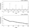 |
Fig. 3 Autocorrelation functions of the two candidates eclipsing binaries of Fig. 1. Top: ACF of the real candidate ECL. Bottom: ACF of the contaminated light curve. Note that by characterizing the stars with the ACF it is possible to distinguish between them. |
The ACF is computed from the interpolated time series. Figure 2 shows the ACF of the light curves of four stars that belong to, according to previous supervised classification (Debosscher et al. 2009), four different classes. By using the ACF, all the stars are represented by vectors of equal length. It is possible to distinguish most of the variability classes, using the ACF. As an alternative to clustering Fourier attributes, we propose to cluster the ACFs. In Fig. 3, the autocorrelations of the two candidates binaries of Fig. 1 are shown. We note that by analyzing both ACFs it is possible to discriminate between them.
2.2. Fourier analysis
As mentioned before, the CoRoT dataset has been analysed using supervised (Debosscher et al. 2009) and unsupervised (Sarro et al. 2009) techniques. The results of these analysis are based on grouping Fourier parameters extracted in an automated way from all the stars. Three frequencies and each of the four harmonics are fitted to the light curves, resulting in a set of Fourier parameters available for clustering and classification. The set of parameters is formed by frequencies, amplitudes, and phases. In those works, several misclassifications were caused by unreliable feature extraction. In other words, some stars (e.g. irregulars) cannot be reliably characterized by the set of attributes.
In this work, we propose to extract more frequencies and more harmonics from the light curves, in order to improve the fitting in most of the cases. The procedure implemented here is an adaptation of the methodology used in Debosscher et al. (2007) and is described below (for details we refer to the original paper).
To correct for systematic trends, a second-order polynomial is subtracted from the light curves. Posterior to this, the frequency analysis is done using Lomb-Scargle periodograms (Lomb 1976; Scargle 1982). Up to 6 frequencies and 20 harmonics can be extracted and fitted to the data using least squares fitting. The selection of the frequencies is done by means of a Fisher-test (F-test) applied to the highest peaks of the amplitude spectrum. By doing this, the highly multi periodic and irregular stars can be characterized by more than three frequencies and four harmonics.
With this approach, the set of attributes is different for all the stars. We can have stars with few attributes (e.g. one frequency, two harmonics, three amplitudes, and two phases) and stars with up to 200 attributes in the case of 6 frequencies, 20 harmonics, amplitudes, and phases. This is indeed a more reliable characterization of the light curves, but the implementation of any clustering algorithm becomes impossible. We recall that the set of attributes must be equal for all the objects in the dataset. However, we use these attributes in a way that we explain in Sect. 3.
2.3. Hidden Markov models
In this section we try to characterize the statistical properties of the time series. One way of modelling time series is by means of HMMs. These models assume that the time series are generated by Markov processes that go through a sequence of hidden states.
Hidden Markov models first appeared in the literature around 1970. They have been applied in different fields, such as speech recognition, bioinformatics, econometrics, among others. In this section, we briefly describe the basis of HMMs, and for more details refer the author to Rabiner (1989), Oates et al. (1999), Jebara & Kondor (2003), and Jebara et al. (2007).
The standard Markov models, although very useful in many fields of applied mathematics, are often too restrictive once one considers more intricate problems. An extension that circumvents some of these restrictions, is the class of HMMs. They are called hidden because the observations are probabilistic functions of certain states that are not known. This is in contrast to the “standard” Markov chain, in which each state is related to an observation. In a HMM, however, information about the underlying process of the states is only available through the effect they have on the observations.
It is important to consider the characteristics of the dataset to be modelled. In this implementation, we assume that the time series are ordered sequences of observations, generated by an underlying process that goes through a sequence of different states that cannot be directly observed. Any time series can be modelled using a HMM but it is necessary to consider the properties of the signal. For example, the dataset studied here contains stationary, non-stationary and noisy time series. In addition, the states of the processes (those operating in stellar atmospheres) are normally unknown. When the time series are sequences of discrete values that are taken from a fixed set and the states of the process are defined, both standard Markov models and discrete models can be used.
The most important assumptions made by this kind of statistical models are: (1) the signals can be characterized as a parametric random process; (2) the parameters of the stochastic process can be estimated; and (3) the process only depends on one independent variable, which in this case is time (Rabiner 1989). For applications where the observed signal depends on two or more independent variables, the approach presented in this work cannot be used.
For a set of N time series  where xn is an ordered sequence in time t = 1,... , Tn, there exists a set of HMMs
  . Each θn is a model that generates the sequence xn with a certain probability, and is defined as θ(π,α,μ,Σ), where πi = p(q0 = i), for i = 1,...,M, represents the initial state probability or prior, which is the probability that the process starts in a given state. In this application, π is a vector of length M that is initialized at random. The matrix α ∈ RM × M contains the transition probabilities of going from state i to state j: αij = p(qt = j | qt − 1 = i). This stochastic matrix is also initialized at random. In this approach, a continuous observation density is considered, and is determined by μ and Σ. The observation density indicates the probability of emitting xt from the ith state and is defined as
 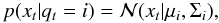 (1)where μi and Σi are respectively the mean and covariance of the Gaussian distribution in state i. The observation density can be composed of a Gaussian mixture, and for this work we consider up to two Gaussian distributions. Figure 4 shows a simple example of a HMM consisting of three states q1, q2, and q3. For illustration purposes, a time series is indicated as well as a sequence of states through which the model was supposed to pass to generate the observations.
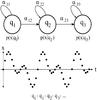 |
Fig. 4 Top: example of a hidden Markov model consisting of three states: q1, q2, and q3. αij represents the probability of going from state i to state j. p(x | qi) is a continuous emission density that corresponds to the probability of emitting x in state qi. Bottom: observations (time series) that the model generated by going through the indicated sequence of states. |
Once the number of states, the prior probability, the transition, and the observation probability matrices are initialized, the expectation-maximization (EM) algorithm, also called Baum-Welch algorithm, is used to estimate the parameters of the HMMs (see Zucchini & MacDonald 2009). The most important assumption of HMM is that the process goes through a sequence of hidden states to generate the observed time series. From this, the EM algorithm performs maximum likelihood estimation with missing data (the states). The algorithm consists of two stages: expectation (E) and maximization (M).
In the E-step, the algorithm estimates the missing data from the observations and the current model parameters. This is why it is necessary to give an initial estimate of the probability matrices and the number of states. Posterior to this, the M-step maximizes the likelihood function defined as 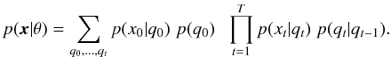 (2)Different models are evaluated (from two to ten states) but the one with the highest likelihood is selected as the model that generates a given sequence.
Once the best-fit model parameters for every time series are selected, the new data consists of N HMMs. The likelihood of every model generating each time series is then computed, and we obtain a new representation of the data. We propose to treat each time series as a point in an N dimensional space, where the value in the nth dimension is determined by the likelihood of the model θn generating the given time series.
3. Kernel spectral clustering
Clustering is an unsupervised learning technique (Jain et al. 1999), that separates the data into substructures called clusters. These groups are formed by objects that are similar to each other and dissimilar to objects in different clusters. Different algorithms use a metric or a similarity measure, to partition the dataset.
Two of the most used clustering algorithms are k-means, defined as a partition, center-based technique, and hierarchical clustering, which is subdivided into agglomerative and divisive methods (Seber 1984). It has been shown that for some of the applications where these classic clustering methods fail, spectral clustering techniques perform better (von Luxburg 2007).
Spectral clustering uses the eigenvectors of a (modified) similarity matrix derived from the data, to separate the points into groups. Spectral clustering was initially studied in the context of graph partitioning problems (Shi & Malik 2000; Ng et al. 2001). It has also been adapted to random walks and perturbation theory. A description of all these applications of spectral clustering can be found in von Luxburg (2007).
The technique used in this work (Alzate & Suykens 2010), kernel spectral clustering, is based on weighted kernel principal component analysis (PCA) and the primal-dual least-squares support vector machine (LS-SVM) formulations discussed in Suykens et al. (2002). The main idea of kernel PCA is to go to a high dimensional space and there apply linear PCA.
We now briefly describe the algorithm that is presented in detail in Alzate & Suykens (2010). For further reading on SVM and LS-SVM, we refer to Vapnik (1998), Schölkopf & Smola (2002), Suykens et al. (2002), and Suykens et al. (2010).
3.1. Problem definition
Given a set of N training data points  , xi ∈ Rd and the number of desired clusters k, we can formulate the clustering model
  (3)where ϕ(·) is a mapping to a high-dimensional feature space and w(l),bl are the unknowns. Cluster decisions are taken by
  , thus the clustering model can be seen as a set of k − 1 binary cluster decisions that need to be transformed into the final k groups. The data point xi can be regarded as a representation of a light curve in a d-dimensional space. The clustering problem formulation we use in this work (Alzate & Suykens 2010) is then defined as
 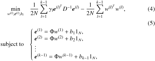 where 1N is the all-ones vector, γl are positive regularization constants, e(l) is the compact form of the projections
 ![Mathematical equation: \hbox{${\vec e}^{(l)}=[{\vec e}^{(l)}_1,\dots,{\vec e}^{(l)}_N]$}](/articles/aa/full_html/2011/07/aa16419-10/aa16419-10-eq48.png) , Φ = [ϕ(x1)T;...;ϕ(xN)T] , and D is a symmetric positive definite weighting matrix typically chosen to be diagonal. This problem is also called the primal problem. In general, the mapping ϕ(·) might be unknown (typically it is implicitly defined by means of a kernel function), thus the primal problem cannot be solved directly. To solve this problem, it is necessary to formulate the Lagrangian of the primal problem and satisfy the Karush-Kuhn-Tucker (KKT) optimality conditions. This reformulation leads to a problem where the mapping ϕ(·) need not to be known. For further reading on optimization theory, we refer to Boyd & Vandenberghe (2004).
, Φ = [ϕ(x1)T;...;ϕ(xN)T] , and D is a symmetric positive definite weighting matrix typically chosen to be diagonal. This problem is also called the primal problem. In general, the mapping ϕ(·) might be unknown (typically it is implicitly defined by means of a kernel function), thus the primal problem cannot be solved directly. To solve this problem, it is necessary to formulate the Lagrangian of the primal problem and satisfy the Karush-Kuhn-Tucker (KKT) optimality conditions. This reformulation leads to a problem where the mapping ϕ(·) need not to be known. For further reading on optimization theory, we refer to Boyd & Vandenberghe (2004).
Alzate & Suykens (2010) proved that the eigenvalue problem satisfies the KKT conditions of the Lagrangian (dual problem)  (6)where λl and α(l) are the eigenvalues and eigenvectors of D-1MDΩ respectively, λl = N/γl, and Ωij = ϕ(xi)Tϕ(xj) = K(xi,xj). The matrix MD is a weighting centering matrix and bl are the bias terms that result from the optimality conditions
  (7)where IN is the identity matrix. The effect of these two terms is to center of the kernel matrix Ω by removing the weighted mean from each column. By centering the kernel matrix, it is possible to use the eigenvectors corresponding to the first k − 1 eigenvalues to partition the dataset into k clusters. After selecting a training set of light curves and defining a kernel function and its parameters1, the matrix D-1MDΩ is created. The eigenvectors α(l) are then computed providing information about the underlying groups present in the training set of light curves. The clustering model in the dual form can be computed by re-expressing it in terms of the eigenvectors α(l)
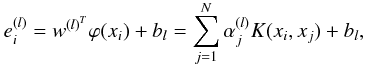 (8)where i = 1,...,N,, and l = 1,...,k − 1. To illustrate this methodology, we manually select 51 stars and we use two Fourier parameters: fundamental frequency and amplitude. Figure 5 shows the dataset, consisting of training and validation sets.
 |
Fig. 5 Top left: dataset. Training set (filled circles) and validation set (crosses). Top right: eigenvectors α(1)(open circles) and α(2)(filled circles) containing the clustering information for the training set. Bottom: Kernel matrices for different σ2 values. The intensity indicates how similar the points are to each other. White indicates that the points should be in the same cluster. From left to right: σ2 = 0.01, σ2 = 0.2, σ2 = 5. Note that for the first case the points are only similar to themselves. In other words, only the points in the diagonal are 1, the rest is approximately zero. For the right case, it is difficult to discriminate between some points, especially in the first two clusters (first two blocks). As the kernel parameter σ2 increases, the model becomes less able to discriminate between the clusters. |
For this particular example, we know that the number of clusters is k = 3, hence the clustering information is contained in the two eigenvectors corresponding to the two highest eigenvalues of Eq. (6). These two eigenvectors, α(1) and α(2), are indicated in Fig. 5.
The kernel function used in this example is the RBF kernel defined as  (9)with a predetermined kernel parameter σ2 = 0.2. The kernel parameter has a direct influence on the partition of the data. When σ2 is too small, the similarity between the points will drop to zero and the kernel matrix will be approximated by the identity matrix. The opposite case occurs when the σ2 is too big, when all the points will then be highly similar to each other. In both extreme situations, the algorithm is unable to distinguish between the clusters correctly. For these reasons, the selection of the kernel parameter needs to be done based on a suitable criterion. In this work, we use balanced line-fit (BLF) criterion as proposed by Alzate & Suykens (2010) and discussed later in this section. Figure 5 indicates three kernel matrices for different σ2 values.
Owing to the piecewise constant structure of the eigenvectors, it is possible to obtain a “codeword” for each point in the training set. This is done by binarizing the eigenvectors using sign , i = 1,...,N, l = 1,...,k − 1. For the example of Fig. 5, the resultant coding is presented in Table 1.
3.2. Extensions to new data points
One of the most important goals of a machine learning technique, is to be able to expand a learned concept to new data. The model should be able to cluster new data. In other words, when new stars are observed, they are automatically associated with the clusters. This is the so-called out-of-sample extension, which is implemented using the projections of the mapped validation points onto the α(l) eigenvectors obtained with the training dataset.
For a validation set of Nv light curves  , a validation kernel matrix
  is computed. This matrix can be seen as a similarity measure between the validation and the training points.
To associate the validation points with the k clusters, the projections onto the α(k − 1) eigenvectors are binarized. A matrix Zv ∈ RNv × (k − 1) is computed, with entries 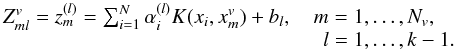 (10)A codeword for each validation point is obtained and compared with the codes discussed before (Table 1), using Hamming distance. In the same way as the training set is partitioned, the validation points are grouped into the k clusters.
The projections  are also used to evaluate the goodness of the model. Figure 6 shows the projections of all the points of the dataset onto the two eigenvectors α(1) and α(2). The alignment of the points in each quadrant indicates how accurately the clusters are formed, which was proposed by Alzate & Suykens (2010) as a model selection criterion. In Fig. 6 (top), one can observe that the colinearity of the points in the clusters is imperfect. This can be changed by tuning the kernel parameter or the number of clusters. The projections for a more suitable σ2 value are shown in the same figure.
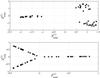 |
Fig. 6 Score variables for the training and validation sets with kernel parameter σ2 = 0.7 (top) and σ2 = 0.1 (bottom). Note that the alignment for the second result is better, thus this is selected as the final model. |
We previously mentioned that special care needs to be taken when selecting a training set. In this work, we use the fixed-size algorithm described in Suykens et al. (2002). With this method, the dimensionality of the kernel matrix goes from N × N to M × M, where M ≪ N. To select the light curves most closely represent the whole dataset, the quadratic Renyi entropy is used and defined as 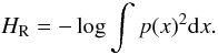 (11)The entropy is related to kernel PCA and density estimation by Girolami (200212) as
 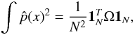 (12)where Ω is the kernel matrix and 1N = [1;1;...;1] . The main idea of the fixed-size method is to find M points that maximize the quadratic Renyi entropy. This is done by selecting M points from the dataset and iteratively replacing them until a higher value of entropy is found. For implementation details, we refer to Suykens et al. (2002).
Algorithm 1 shows the kernel spectral clustering technique, described above. More information about the implementation can be found in Alzate & Suykens (2010).
| Algorithm 1. Kernel spectral clustering |
|
|
Input: Dataset  , with
NT the total number of time series,
positive definite kernel function
K(xi,xj),
number of clusters k, , with
NT the total number of time series,
positive definite kernel function
K(xi,xj),
number of clusters k, |
Output: Partition  . . |
1. We select N points that maximize the quadratic Renyi entropy defined in Eq. (11). These points correspond to the training set . From the NT − N points left, we extract the validation set  . . |
| 2. We calculate the training kernel matrix Ωij = K(xi,xj), i,j = 1,...,N. |
| 3. We next compute the eigendecomposition of D-1MDΩ, indicated in Eq. (6). Obtaining the eigenvectors α(l) where l = 1,...,k − 1, which correspond to the largest k − 1 eigenvalues. |
| 4. We binarize the eigenvectors α(l) and obtain sign, where i = 1...,N and l = 1,...,k − 1. |
5. We obtain from sign the encoding for the training set. We find the k most frequent encodings that will form the codeset:  , cp ∈ {−1,1 } k − 1. , cp ∈ {−1,1 } k − 1. |
6. We compute the Hamming distance dH(.,.) between the code of each xi, namely sign(αi), and all the codes in the codeset  . We select the code cp with the minimum distance and assign xi to . We select the code cp with the minimum distance and assign xi to  where p ⋆ = argmin where p ⋆ = argmin sign(αi),cp). sign(αi),cp). |
7. We then binarize the projections of the validation set, sign , m = 1,...,Nv, defined in Eq. (10). We define sign(zm) to be the encoding vector of , m = 1,...,Nv, defined in Eq. (10). We define sign(zm) to be the encoding vector of  . . |
| 8. Using p ⋆ = argminsign(zm),cp), and for all m, we assign to . |
4. Experimental results
The three different characterizations (Fourier attributes, ACFs, and HMMs) described above are studied using kernel spectral clustering2. We use the RBF kernel because it is a localized and positive definite kernel, which ensures that it is a good choice as a similarity measure in the context of spectral clustering. For each implementation, the most suitable model is selected using the BLF criterion. Once each model is selected, an analysis of the eigenvectors is performed.
With the BLF criterion, we select the most likely values of the kernel parameter and the number of clusters. This model then corresponds to the final solution using kernel spectral clustering with a particular characterization. In other words, we obtain three different sets of k and σ2, one for clustering Fourier attributes, another of ACFs, and a last one for HMMs. These three different clustering results are compared using the silhouette index (see Rousseeuw 1987), which is a well-known internal validation technique, used in clustering to interpret and validate clusters of data. This index, used to find the most accurate clustering of the data is described as follows. The silhouette value S(i) of an object i, measures how similar i is to the other points in its own cluster. It takes values from − 1 to 1 and is defined as  (13)or equivalently
  (14)where a(i) is the average distance between point i and the other points in the same cluster, i = 1,...,nk, nk being the number of points in cluster k, and b(i) is the lowest average distance between point i and the points in all the other clusters. When S(i) is close to 1, the object i is assigned to the right cluster, when S(i) = 0 then i can be considered as an intermediate case, and when S(i) = −1, the point i is assigned to the wrong cluster. Hence, if all the objects in the dataset produce a positive silhouette value, this indicates that the clustering results are consistent with the data. To compare two different results, it is necessary to compute the average silhouette values, and the results with the highest value are then selected as the most appropriate clustering of the data.
Other validation methods exist, such as the Adjusted Rand Index (Hubert & Arabie 1985). This is an external validation technique that uses a reference partition to determine how closely the clustering results are related to a desired classification. This index ranges between − 1 and 1 and takes the value of 1 when the cluster indicators match the reference partition. In applications such as this one, where stars were observed for the first time, it is not possible to have a reference partition. The closest reference we have is the partition generated by supervised classification in Debosscher et al. (2009). This is not an accurate reference because there are some limitations in this supervised approach, such as an incomplete characterization of the time series, adding errors to this reference classification. However, there are some light curves that have been manually classified, which we use as a reference, to compare the different results. At the end of this section, we present these candidates and the partition obtained with different methods.
To determine whether our results are more reliable than those obtained by basic clustering techniques, we run k-means and hierarchical clustering on the Fourier attributes extracted by Debosscher et al. (2009). These results will be later compared with those obtained after using kernel spectral clustering.
4.1. k-means and hierarchical clustering
It is first necessary to find the most relevant Fourier attributes from the set extracted by Debosscher et al. (2009). We do this by first selecting seven classes, defined in the supervised approach, namely: variable Be-stars (BE), δ Scuti (δ Sct), ellipsoidal variables (ELL), short period δ Scuti (SPDS), slowly pulsating Be-stars (SPB), eclipsing variables (ECL), and low amplitude periodic variables (LAPV). After selecting those classes, we find the set of attributes that most closely reproduce these seven groups using clustering techniques. We run k-means with different distance measurements, and hierarchical clustering with several linkage methods. For details of these algorithms, we refer to Seber (1984). Each algorithm is implemented for different sets of attributes, and each one produces different clustering results that we compare with the supervised classification of Debosscher et al. (2009) using the adjusted rand index mentioned before. This index takes a value of 1 when the cluster indicators match the reference partition which corresponds in this case to the seven classes found by the supervised approach of Debosscher et al. (2009).
The maximum ARI obtained is 0.3267, which is produced by the k-means algorithm using Euclidean distance on the following set of attributes  where A11 and A21 correspond to the amplitude of the first and second most significant frequencies respectively, and A12 and A22 are the amplitudes of the second harmonics of the two significant frequencies. This set of attributes, together with the amplitudes of the third and fourth harmonics of f1 was also used in Sarro et al. (2009).
Once the best set of attributes and algorithm are selected, we perform clustering on the dataset and evaluate the clustering results for different values of k, using the silhouette index. The goal is to find the number of clusters that produce the best partition of the data. This corresponds to k = 8, for an average silhouette of 0.2325. This silhouette value indicates that more than half of the light curves are associated with the correct cluster. Figure 7 shows the distribution of the clusters in the plane log f1–log f2.
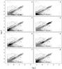 |
Fig. 7 Clusters obtained applying k-means algorithm to log f1, log f2, log A11, log A12, log A21, and log A22. Results for k = 8. The clusters are indicated in black. |
After this first clustering implementation, we compare the results with those of Debosscher et al. (2009) and Sarro et al. (2009), and it is already possible to discriminate the “obvious” classes. For example, cluster 7 contains mainly eclipsing binaries, cluster 6 is formed by SPB, γ Dor, and some ECL candidates, and some light curves in cluster 4 can be assigned to the δ Sct class. Cluster 4 also contains some SPB candidates. Cluster 2 contains light curves that show some monoperiodic variations. This cluster as well as clusters 3, 5, and 8 contain stars for which the light curves indicate rotational modulation and variations in the type of Be stars. Cluster 1 contains candidates δ Sct for which the second frequency is significantly lower. This cluster contains highly contaminated light curves and SPB candidates. The separation of the SPB, δ Sct, and γ Dor can be done by using temperature information or color indices such as B − V. A greater problem is the separation of the contaminated light curves, some binary systems, and irregular variables. We recall that k-means clustering finds linearly separable clusters. In addition, the characterization of the light curves is done using Fourier analysis. This is why we go to higher dimensional spaces, by means of a kernel function (RBF), and apply a more sophisticated clustering algorithm. These results are presented as follows.
For all the implementations, it is necessary to define a grid with the two model parameters, namely number of clusters k and kernel bandwidth σ. In Debosscher et al. (2009), 30 variability classes were considered for the training set, hence taking this assumption into account, k takes values between 25 and 34 clusters. The range for the kernel parameter is defined to be around a value (rule of thumb) corresponding to the mean of the variance in all dimensions, multiplied by the number of dimensions in the dataset.
Owing to the large-scale aspect of the dataset, namely about 28 000 stars, it is practically impossible to store a kernel matrix of this size. For this reason, it is necessary to select a subset that most accurately represents the underlying distribution of the objects in the dataset. On the basis of the size of the largest matrix that can be used in the development environment (MATLAB), namely 2000 × 2000, we select 2000 light curves as a training set. It is important to keep in mind that this training set differs significantly from the one used in supervised classification. In the last case, the training set contains inputs and the desired output, from which the model learns. In our implementation, we reduce the size of the dataset that is used to train a model, which is later tuned with a validation set. No output is predefined and the model is learned in a complete unsupervised way. For this unsupervised implementation, it is important to include in the training set, light curves of all types. The way we guarantee this is by selecting the most dissimilar light curves of the dataset. Hence, this procedure cannot be done at random; if this were the case, then the large dataset would not be correctly characterised.
The training set is selected using the fixed-size algorithm proposed in Suykens et al. (2002). A validation set consisting of 4000 light curves is also selected. We mentioned before that the limiting size for a matrix in our implementation is 2000 × 2000. This corresponds to the maximum matrix size that we can use to obtain an eigendecomposition. For the validation set, we do not need to do this, and this is why we can select (for practical reasons) 4000 light curves.
To visualize the training set, we plot in Fig. 8 the Fourier parameters computed in Debosscher et al. (2009). We note that the support vectors (training examples) represent the underlying distribution of the points in the Fourier space formed by the fundamental frequency and its amplitude.
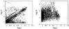 |
Fig. 8 Training set (black) compared with the dataset. The logarithm of the Fourier attributes is plotted, where f1 is the fundamental frequency, f2 the second significant frequency, and A1 the amplitude of the fundamental frequency. Note that the training examples describe the underlying distribution of the dataset. |
4.2. Kernel spectral clustering of autocorrelation functions
The first approach consists of the clustering the ACFs. After evaluating the BLF with different model parameters, the highest value corresponds to k = 27 and σ2 = 360. One important and useful result is that the binary systems are clustered in a separate group. In Fig. 9, three examples of four different clusters are indicated. We include the two ACFs of the two ECL candidates presented in Fig. 1. In this approach, those two light curves are associated with two different clusters. The ACFs of the real eclipsing candidate is indicated in the fourth row and third column of the figure, while the contaminated one is associated with cluster 2 (second row) and indicated in the third column.
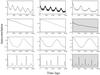 |
Fig. 9 Some clustering results obtained with ACFs. Each row indicates one cluster. In the third column, second row, the ACF of the contaminated light curve of Fig. 1 is indicated. The real eclipsing binary of that example is associated with another cluster (fourth row and third column). |
From the results produced by the spectral clustering of ACFs, it is already possible to improve the classification of binary stars. After validating the results, it is observed that the mean silhouette value is −0.196. This indicates that the partition is incompatible with the data, or in other words, more than 50% of the light curves are associated with the wrong cluster. This is probably related to another important observation, namely that the amplitude information is lost when taking the ACF. This is a significant drawback because we are interested in detecting variability classes that differ not only in frequency range, but also in the amplitude of the oscillations. This brings us to the second characterization, namely the Fourier parameters.
4.3. Kernel spectral clustering of Fourier parameters
In Sect. 2, a variable set of parameters was extracted from each light curve. The different sets cannot be directly compared using clustering, because the dimensions of the points have to be the same. We propose to create a new attribute space, formed by the number of frequencies extracted from the data, together with the number of harmonics of the fundamental frequency, the fundamental frequency, and its amplitude. This results in a 4-dimensional space. We select these attributes based on the assumption that most of the stars are periodic and that at least one frequency was extracted from all of the time series. It is clear that other combinations of Fourier attributes could produce more reliable results, but that the set of parameters must be fixed, corresponding to an incomplete characterisation of some of the light curves in the dataset.
After using the 4-dimensional space described above, this approach produces a mean silhouette value of −0.437, which is a poor result. In other words, the majority of the light curves in most of the clusters are significantly dissimilar to each other.
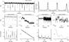 |
Fig. 10 Top: light curve (left) and ACF (right) of a candidate ECL that is used to train a HMM. The other two rows indicate the light curves (middle), and its autocorrelations (bottom), of four objects, two in the training set (101551987 and 101344332) and two in the validation set (211665710 and 101199903). |
4.4. Kernel spectral clustering of hidden Markov models
The last characterization corresponds to that produced by the HMM. To train the HMM, we use the toolbox of HMMs for Matlab, written by Murphy (1998). In this implementation, models between two and ten hidden states are tested. The likelihood of each time series is computed using the EM algorithm. A compromise must be made in the selection of the maximum number of states. It is possible that some time series will be more accurately represented by a model with more than ten states, but it is also possible that this time series will be overfitted by those particular models. The number of states is an important parameter, and needs to be optimized to achieve the maximum performance. However, in this implementation we did not optimize this number, instead we tested different number of states and ten appears to be an acceptable upper limit.
Figure 10 shows an example of a light curve (CoRoT 101166793) that belongs to the training set. This light curve is used to train a HMM. As mentioned before, each HMM of the training set is used to compute the likelihood to generate all the light curves in the training and validation sets. The negative logarithm of the likelihood obtained for this time series is –97.7430. In the figure, four different light curves are also indicated, two of them belonging to the training set (101551987 and 101344332) and the other two (211665710 and 101199903) to the validation set. The negative logarithm of the likelihoods for these four light curves are −197.64, −2.599 × 10³, −230.4267, and −3.1532 × 10³, respectively. It is already possible to observe that the similarity between the binary stars is captured by this approach, as well as with the clustering of ACFs.
Once the matrix containing all the logarithms of the likelihoods is computed, an RBF kernel is used. A grid is defined, where k ranges from 3 to 40 clusters, and the kernel parameter σ2 takes values between 1.4325 × 10¹⁰ and 1.4325 × 10¹². The BLF criterion is used to select the optimal set of parameters, as shown In Fig. 11 for different values of k and σ2. As mentioned earlier in this section, we are interested in finding clusters in the range between 25 and 34. For completeness, however, we also show the BLF values for k ranging from 3 to 40 clusters in Fig. 11(left). Here one can see that the two highest values correspond to k = 8 and k = 31. To compare these two results, we use the light curves that were manually classified. In this case, we can rely on the adjusted rand index (ARI) that was described at the beginning of this section. The ARI for k = 8 is 0.4853, and for k = 31 it is 0.5570. This indicates that the light curves are more closely associated when k = 31. In addition, we already know that this kind of dataset can be divided into more than 25 groups (Debosscher et al. 2009). The best-fit model then corresponds to k = 31 and σ2 = 1.3752 × 10¹² with a BLF value of 0.8442.
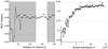 |
Fig. 11 Model selection for the clustering of HMM of the CoRoT dataset. The non-shaded area in the left indicates our region of interest. The selected model corresponds to k = 31 (left) and σ2 = 1.3752 × 10¹² (right) with a BLF value of 0.8442. |
Using the clustering results produced by the model with the set of parameters selected above, the mean silhouette value obtained for this implementation is 0.1658, which is better than the one obtained with the ACFs (−0.196).
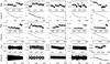 |
Fig. 12 Light curves and ACFs assign to cluster 3 (rows 1 and 2). The corot identifiers are (from left ro right): 211637023, 211625883, 102857717, 102818921, and 100824047. This cluster as well as cluster 5 (rows 3 and 4) contains contaminated light curves that are classified as PVSG, CP and MISC by supervised techniques. The identifiers for cluster 5 are (from left ro right): 102860822, 102829101, 211635390, 211659499, and 102904547. Cluster 6 (last two rows) consists mainly of DSCT and SPDS. The CoRoT IDs for these examples are: 102945921, 102943667, 101286762, 101085694, and 211657513. The abscissas of the odd rows is indicated in HJD (days) and of the even ones in time lags. |
By manually checking the clusters, it is possible to find results that can improve the accuracy of a catalogue, as discussed below. It is important to keep in mind that our purpose is not to deliver a catalogue, but rather as mentioned at the beginning of this paper, to improve the characterization of the stars and apply a new spectral clustering algorithm to the CoRoT dataset.
In total, 6000 light curves were used to train and validate the model. Fifteen out of 31 clusters have a mean silhouette value larger than zero, and we now discuss the most important characteristics of these clusters.
We analyse the clusters that are well formed according to the silhouette index, which are the clusters with the highest average silhouette value. To start with, cluster 3 contains light curves that indicate that there is contamination caused by jumps. Some examples of light curves in this cluster are indicated in Fig. 12. According to supervised analysis, some of these light curves are classified as DSCUT, PVSG, CP, and MISC (miscellaneous class). This is an important cluster, because some of the light curves with jumps are detected and associated with this cluster. Some other clusters contain this kind of light curves. This brings us to the second well-formed cluster according to the silhouette index. Cluster 5 contains only contaminated light curves, which were classified as PVSG and LBV candidates by supervised techniques. Cluster 6 contains mainly DSCT and SPDS candidates. Some other light curves associated with this cluster were classified as CP candidates. Examples of these two clusters are also indicated in Fig. 12.
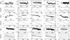 |
Fig. 13 Light curves and ACFs assign to cluster 7 (rows 1 and 2). The corot identifiers are (from left ro right): 211656935, 102765765, 102901628, 211633836, and 211645959. This cluster contains pulsating, monoperiodic variables. Cluster 8 (rows 3 and 4) contains contaminated light curves, classified by supervised techniques as PVSG, CP. The identifiers for cluster 8 are (from left ro right): 101518066, 101433441, 101122587, 110568806, and 101268486. Cluster 10 (last two rows) contains mainly monoperiodic variables. The CoRoT IDs for these examples are: 102760966, 211607636, 100521116, 100723479, and 211650240. The abscissas of the odd rows is indicated in HJD (days) and of the even ones in time lags. |
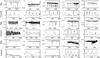 |
Fig. 14 Light curves and ACFs assign to clusters 12, 13, and 23. The corot identifiers are (from top to bottom, left ro right): 211663851, 102901962, 100966880, 102708916, 211612920, 211659387, 102918586, 211639152, 102776565, 102931335, 102895470, 102882044, 102733699, 102801308, and 100707214. The abscissas of the odd rows is indicated in HJD (days) and of the even ones in time lags. All these light curves correspond to candidates ECL. Note also that stars with intrinsic variability are associated with these clusters. For example, 102918586 (Col. 1, row 3) was classified by Debosscher (2009) as a Be candidate. |
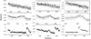 |
Fig. 15 Light curves associated with cluster 15–16, 19, and 27, indicated in rows 1, 2, and 3 respectively. The first row shows examples of light curves in clusters 15 and 16, which contain pulsating variables. Cluster 19 (second row) is formed by light curves with long-term variations. The light curves assigned to the last cluster are contaminated. |
Continuing with the “well formed” clusters, we analyse cluster 7. This cluster contains light curves of different classes. We note that we do not use frequency information, hence it is unsurprising that overlap between classes, with different oscillation periods, is present. As mentioned before, cluster 7 corresponds to light curves of a different kind, namely pulsating and monoperiodic variables. Some time series in this cluster have been classified as CP candidates, which are difficult to identify by only using photometric information (Debosscher 2009). Some Be stars are also observed in this cluster together with some LAPV candidates. Figure 13 shows some light curves associated with this cluster.
Cluster 8 contains 270 contaminated and irregular light curves that are mainly classified as PVSG and CP candidates. Examples for this cluster are indicated in Fig. 13. Cluster 10 is formed by SPB and SPDS candidates. Multiperiodicity is the common characteristic of the light curves in this cluster and also in cluster 11. Some examples of SPB and SPDS in this cluster are shown in Fig. 13.
Clusters 12, 13, and 23 contain eclipsing binary candidates. Some examples of light curves in these clusters are shown in Fig. 14. Some light curves indicate clear eclipses, while others, such as the ones indicated in the figure, show intrinsic and extrinsic variability. These stars cannot be clearly classified using supervised techniques or k-means. Taking as an example the light curve with the identifier 211659387, shown in the figure in the first column and third row. This object was classified as a DSCT candidate by the supervised algorithm, while it is clearly visible that it is an eclipsing binary candidate. This is a significant improvement compared with previous analysis on CoRoT. We note that light curves with few eclipses are also associated with the cluster corresponding to the ECL candidates. This is another important contribution of this work.
Clusters 15 and 16 (see Fig. 15) contain light curves of pulsating variables. Some Be candidates are found in these two clusters. SPB candidates are also found in cluster 16, together with light curves that have been classified as PVSG before. In Fig. 15, examples of light curves associated with cluster 19 are indicated. Some of them were classified before (Debosscher 2009) as SPDS, γ Dor, and PVSG. Light curves in this cluster present long-term variations. The last cluster indicated in the figure, namely cluster 27, contains mainly contaminated light curves. Another cluster with a positive silhouette value is the number 26. This cluster contains SPB candidates and some other stars that have similar variability but were classified as ECL. A specific example is the light curve with identifier 211663178.
The remaining clusters contain a mixture of pulsating, multiperiodic or monoperiodic variables. We attempted to distinguish the contaminated light curves, 602 out of 6000 light curves being associated with clusters 3, 5, 6, 8, and 27. Figure 16 shows the ACFs of the light curves associated with these clusters. For visualization purposes, we plot only clusters 3, 5, 6, and 27.
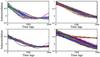 |
Fig. 16 ACFs of examples in clusters (from top to bottom, left to right) 3, 5, 6 and 27. All the light curves associated to these clusters present jumps. |
After studying the clusters separately, we can conclude that the contaminated light curves could be clearly separated. However, when the contamination does not affect significant regions in the light curve, it is still possible to associate the object with one of the clusters with real variable candidates. The second stage of our analysis was then to distinguish the binary systems. Even when the host star displays different kinds of oscillations or when only one eclipse was observed, we are able to separate those from the contaminated and the other candidates. Once the contaminated light curves are separated from the rest, it is possible to implement cleaning techniques, such as the one developed by Degroote et al. (2009a). If the binary systems are separated from the ones with highly contaminated light curves, it is safer to clean the time series without affecting either intrinsic or extrinsic oscillations.
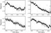 |
Fig. 17 Light curves associated to cluster 29. Using frequency analysis it is difficult to characterize this kind of stars. With our method, we can separate them. |
The last important result is that the irregular variables are separated from the periodic ones. Cluster 29 contains only this kind of stars and allows us to treat them in a different way from the periodic ones. This is a significant advantage because methods such as Fourier analysis do not produce a good characterization of this type of stars and we are able to separate 509 light curves that have irregular properties. Hence, the automated methods always associate these stars with the wrong group. Figure 17 indicates some examples of light curves assigned to this cluster.
Manual comparison of three different methods.
To confirm that the results obtained with this implementation are due to the combination of the new characterization of the light curves with the kernel spectral clustering algorithm, we apply k-means to the likelihood matrix. The best result obtained with k-means corresponds to k = 27 and produces an average silhouette value of 0.0324. The partition obtained does not help us to discriminate between the eclipsing binaries and the multiperiodic variables. However, the association of the contaminated light curves with a separate cluster is also obtained with this basic clustering algorithm. This confirms that the new characterization provides a way of improving the automated classification of variable stars. The separation of the irregular light curves is no longer possible with this simple approach, hence we obtained most of our results here using the kernel spectral clustering algorithm.
As mentioned at the beginning of this section, a manually classified set (test set) of light curves is used to compare different results, namely the ones obtained with supervised classification, HMM+kernel spectral clustering, and HMM+k-means. The test set contains eclipsing binary candidates, contaminated light curves, and irregular variables. Some of the objects in this set correspond to the most problematic light curves in Debosscher et al. (2009) and this is why we include them in this test set. In Table 2, we present the number of light curves used for this comparison. We indicate the number of objects per class and the percentage that is correctly distinguished by each of the methods that are compared. The table lists for each class (binary, contaminated, and irregular) the number of light curves associated with a particular group.
Forty binaries were selected, and in Debosscher et al. (2009) nine of them were classified as eclipsing binary candidates, the remainder being associated with classes such as RVTAU, CP, BE, PVSG, LAPV, and WR. HMM+k-means assigned these binaries to nine different clusters. The best result was obtained with HMM+KSC, where 36 light curves were associated with clusters 12, 13, and 23, corresponding to the eclipsing binary candidates. Only 4 light curves were assigned to different clusters.
Forty irregular light curves were also selected. The supervised classification approach assigned them to different classes, as shown in Table 2. The implementation of HMM+k-means divides them into 6 different clusters, while HMM+KSC groups 37 of them in cluster 29, which we characterized as the cluster of irregular variables. As a final reference, we use 42 contaminated light curves. The results produced by supervised classification and HMM+k-means indicate that these kinds of light curves are associated with several classes or clusters, respectively. With HMM+KSC, these light curves are assigned to clusters 27, 5, 6, and 3. With this test set, we can see that k-means separates these three classes into 20 clusters, without counting the clusters with only one light curve. In contrast, HMM+KSC separates them into 9 clusters out of 31.
5. Conclusions
We have presented the results of applying a new spectral clustering technique to three different characterizations of the CoRoT light curves, namely by means of Fourier parameters, ACF of the light curves, and hidden Markov models of the time series. A brief description of these formalisms has been presented, along with an explanation of the clustering algorithm that is implemented.
To summarize, the Fourier parameters are extracted by means of harmonic fitting techniques. A variable set of Fourier attributes is extracted from the time series. This set is later used to define an attribute space that is used to cluster the stars. This particular implementation does not produce good results but does provide a closer fitting of the light curves, hence more reliable characterization of the stars. These attributes can be combined with a different set, for example either ACFs or HMMs, to improve the results.
The ACFs of the time series were used to cluster the stars. We proposed differentiating between ACFs instead of comparing time series. Some important results were obtained, such as the separation of the contaminated light curves from the eclipsing binaries. This becomes important when one wishes to remove noise from the light curves without affecting the dynamics of the ECL. The results produced by clustering the ACFs are not satisfactory. Therefore, a third implementation is performed, namely the modelling of the stars using HMMs.
Each time series is modelled by a HMM, and the pairwise likelihood is computed for all the time series and models. We propose to use the likelihoods as a new attribute space defining the stars. The spectral clustering algorithm produces significantly more reliable results than those of the ACFs.
Our most important results are summarized as follows:
-
We succeeded in identifying the irregular variables: this allowsus to treat this kind of stars in a different way from periodic stars.The inclusion of these light curves in the dataset, alwaysincreased the misclassifications in previous analyses of theCoRoT dataset.
-
We identified the light curves with high contamination: as soon as these time series were separated from the rest, it is possible to filter them or to apply different cleaning techniques, without affecting intrinsic or extrinsic oscillations.
-
We clearly distinguished the binary systems, a result that can be also used for detecting planetary transits. 322 out of 6000 light curves were assigned to the clusters of binary candidates.
-
We performed a new and more accurate characterization of the light curves.
Other techniques exist to characterize light curves, such as ARIMA models and wavelet analysis. However, some improvements can still be implemented to the HMM approach presented in this work. One of them is the combination of attribute spaces, which can be done by combining three kernels (Fourier+ACF+Time series). Another improvement can be obtained by changing the kernel matrix from RBF to likelihood kernels or including dynamic time warping (DTW). A different kernel function can detect similarities between the light curves, which cannot be found with the method used in this work.
Since there is already some knowledge of this kind of datasets, it is possible to include some constraints in the clustering algorithm (Alzate & Suykens 2009). Constrained clustering is an important tool that improves the accuracy of the partitions thanks to the inclusion of prior knowledge. In addition, it is possible to specify that two light curves should or should not be assigned to the same cluster.
The methodology that we have presented in this paper can be applied to any dataset consisting of time series. In case one needs to cluster images or spectra, it is important to determine how well the RBF kernel performs for each particular application. In addition, the HMM present some limitations. As mentioned in Sect. 2.3, the dataset needs to have particular properties to be modelled with HMMs.
For some datasets, it will not be necessary to use this sophisticated methodology, for instance where the clusters are linearly separable, and can be analysed using basic clustering algorithms such as k-means and hierarchical clustering. For example, when only periodic variables are analysed it is sufficient to characterise the light curves using Fourier parameters and cluster them using k-means. However, it is always difficult to anticipate the kinds of objects in a given dataset, especially when they are observed for the first time. Therefore, we need to compare different methodologies in order to select the characterisation that best suits the dataset, and determine the most suitable method for identifying clusters in the dataset.
The selection of a training set and the model parameters requires special care and will be discussed in the next section.
The code is publicly available at: http://www.esat.kuleuven.be/sista/lssvmlab/AaA
Acknowledgments
This work was partially supported by a project grant from the Research Foundation-Flanders, project “Principles of Pattern set Mining”; Research Council KUL: GOA/11/05 Ambiorics, GOA/10/09 MaNet, CoE EF/05/006 Optimization in Engineering(OPTEC), IOF-SCORES4CHEM, several PhD/postdoc and fellow grants; Flemish Government: FWO: PhD/postdoc grants, projects: G0226.06 (cooperative systems and optimization), G0321.06 (Tensors), G.0302.07 (SVM/Kernel), G.0320.08 (convex MPC), G.0558.08 (Robust MHE), G.0557.08 (Glycemia2), G.0588.09 (Brain-machine) research communities (WOG: ICCoS, ANMMM, MLDM); G.0377.09 (Mechatronics MPC) IWT: PhD Grants, Eureka-Flite+, SBO LeCoPro, SBO Climaqs, SBO POM, O and O-Dsquare; Belgian Federal Science Policy Office: IUAP P6/04 (DYSCO, Dynamical systems, control and optimization, 2007–2011); EU: ERNSI; FP7- HD-MPC (INFSO-ICT-223854), COST intelliCIS, FP7-EMBOCON (ICT-248940); Contract Research: AMINAL; Other:Helmholtz: viCERP, ACCM, Bauknecht, Hoerbiger; Research Council of K.U. Leuven (GOA/2008/04); The Fund for Scientific Research of Flanders (G.0332.06), and from the Belgian federal science policy office (C90309: CoRoT Data Exploitation). Carolina Varon is a doctoral student at the K.U. Leuven, Carlos Alzate is a Postdoctoral Fellow of the Research Foundation – Flanders (FWO), Johan Suykens is a professor at the K.U. Leuven and Jonas Debosscher is a Postdoctoral Fellow at the K.U. Leuven, Belgium. The scientific responsibility is assumed by its authors.
References
- Aerts, C., Christensen-Dalsgaard, J., & Kurtz, D. W. 2010, Asteroseis. Astron. Astrophys. Lib. (Springer) [Google Scholar]
- Alzate, C., & Suykens, J. A. K. 2009, in 2009 International Joint Conference on Neural Networks (IJCNN09), 141 [Google Scholar]
- Alzate, C., & Suykens, J. A. K. 2010, IEEE Trans. Pattern Anal. Mach. Intell., 32, 335 [CrossRef] [PubMed] [Google Scholar]
- Auvergne, M., Bodin, P., Boisnard, L., et al. 2009, A&A, 506, 411 [NASA ADS] [CrossRef] [EDP Sciences] [Google Scholar]
- Blomme, J., Debosscher, J., De Ridder, J., et al. 2010, ApJ, 713, L204 [Google Scholar]
- Borucki, W. J., Koch, D., Basri, G., et al. 2010, Science, 327, 977 [NASA ADS] [CrossRef] [PubMed] [Google Scholar]
- Boyd, S., & Vandenberghe, L. 2004, Convex Optimization (Cambridge University Press) [Google Scholar]
- Cheeseman, P., Kelly, J., Self, M., et al. 1988, in Proceedings of the Fifth International Conference On Machine Learning (Morgan Kaufmann Publishers), 54 [Google Scholar]
- Debosscher, J. 2009, Ph.D. Thesis, Katholieke Universiteit Leuven [Google Scholar]
- Debosscher, J., Sarro, L. M., Aerts, C., et al. 2007, A&A, 475, 1159 [NASA ADS] [CrossRef] [EDP Sciences] [Google Scholar]
- Debosscher, J., Sarro, L. M., López, M., et al. 2009, A&A, 506, 519 [NASA ADS] [CrossRef] [EDP Sciences] [Google Scholar]
- Degroote, P., Aerts, C., Ollivier, M., et al. 2009a, A&A, 506, 471 [NASA ADS] [CrossRef] [EDP Sciences] [Google Scholar]
- Degroote, P., Briquet, M., Catala, C., et al. 2009b, A&A, 506, 111 [NASA ADS] [CrossRef] [EDP Sciences] [Google Scholar]
- Eyer, L., & Blake, C. 2005, MNRAS, 358, 30 [NASA ADS] [CrossRef] [Google Scholar]
- Fridlund, M., Baglin, A., Lochard, J., & Conroy, L. 2006, in The CoRoT Mission Pre-Launch Status – Stellar Seismology and Planet Finding [Google Scholar]
- Girolami, M. 2002, Neural Computation, 14, 1455 [CrossRef] [Google Scholar]
- Hojnacki, S. M., Micela, G., LaLonde, S., Feigelson, E., & Kastner, J. 2008, Statis. Meth., 5, 350 [CrossRef] [Google Scholar]
- Hubert, L., & Arabie, P. 1985, J. Classif., 2, 193 [Google Scholar]
- Jain, A. K., Murty, M. N., & Flynn, P. J. 1999, ACM Computing Surveys, 31, 264 [Google Scholar]
- Jebara, T., & Kondor, R. 2003, in Proceedings of the 16th Annual Conference on Computational Learning Theory, COLT 2003, and the 7th Kernel Workshop, Kernel (Springer) 2777, 57 [Google Scholar]
- Jebara, T., Song, Y., & Thadani, Y. 2007, in Machine Learning: ECML 2007, 164 [Google Scholar]
- Lomb, N. R. 1976, Ap&SS, 39, 447 [NASA ADS] [CrossRef] [Google Scholar]
- Murphy, K. 1998, Hidden Markov Model (HMM) Toolbox for Matlab, http://www.cs.ubc.ca/~murphyk/Software/HMM/hmm.html [Google Scholar]
- Ng, A., Jordan, M., & Weiss, Y. 2001, Advances in Neural Information Processing Systems, 14, 849 [Google Scholar]
- Oates, T., Firoiu, L., & Cohen, P. R. 1999, in Proceedings of the IJCAI-99 Workshop on Neural, Symbolic and Reinforcement Learning Methods for Sequence Learning, 17 [Google Scholar]
- Rabiner, L. R. 1989, in Proc. IEEE, 257–286 [Google Scholar]
- Rousseeuw, P. J. 1987, J. Comput. Appl. Mathem., 20, 53 [Google Scholar]
- Roxburgh, I. W., & Vorontsov, S. V. 2006, MNRAS, 369, 1491 [NASA ADS] [CrossRef] [Google Scholar]
- Sarro, L. M., Debosscher, J., Aerts, C., & López, M. 2009, A&A, 506, 535 [NASA ADS] [CrossRef] [EDP Sciences] [Google Scholar]
- Scargle, J. D. 1982, ApJ, 263, 835 [NASA ADS] [CrossRef] [Google Scholar]
- Schölkopf, B., & Smola, A. J. 2002, Learning with Kernels (The MIT press) [Google Scholar]
- Seber, G. A. F. 1984, Multivariate Observations (John Wiley & Sons) [Google Scholar]
- Shi, J., & Malik, J. 2000, IEEE Trans. Pattern Anal. Machine Intell., 22, 888 [Google Scholar]
- Suykens, J. A. K., Van Gestel, T., De Brabanter, J., De Moor B., & Vandewalle J. 2002, Least Squares Support Vector Machines (World Scientific Publishing Co. Pte. Ltd.) [Google Scholar]
- Suykens, J. A. K., Alzate, C., & Pelckmans, K. 2010, Statistics Surveys, 4, 148 [CrossRef] [Google Scholar]
- Vapnik, V. 1998, Statistical learning Theory (John Wiley & Sons, Inc.) [Google Scholar]
- von Luxburg, U. 2007, Statistics and Computing, 17, 395 [Google Scholar]
- Zucchini, W., & MacDonald, I. L. 2009, Monographs on Statistics and Applied Probability, 110, Hidden Markov Models for time series: An introduction using R, 2nd edn. (CRC Press) [Google Scholar]
All Tables
All Figures
|
Fig. 1 Two eclipsing binaries (ECL) candidates obtained by supervised classification (Debosscher et al. 2009) and k-means on the fixed set of Fourier attributes. Top: real candidate ECL. Bottom: contaminated light curve. |
| In the text | |
|
Fig. 2 Autocorrelation function of four CoRoT light curves. Top: original light curves. Bottom: ACFs. The light curves correspond to candidates of four different classes, namely (from left to right), ellipsoidal variable (ELL), short period δ Scuti (SPDS), eclipsing binary (ECL), and β Cephei (BCEP). |
| In the text | |
|
Fig. 3 Autocorrelation functions of the two candidates eclipsing binaries of Fig. 1. Top: ACF of the real candidate ECL. Bottom: ACF of the contaminated light curve. Note that by characterizing the stars with the ACF it is possible to distinguish between them. |
| In the text | |
|
Fig. 4 Top: example of a hidden Markov model consisting of three states: q1, q2, and q3. αij represents the probability of going from state i to state j. p(x | qi) is a continuous emission density that corresponds to the probability of emitting x in state qi. Bottom: observations (time series) that the model generated by going through the indicated sequence of states. |
| In the text | |
|
Fig. 5 Top left: dataset. Training set (filled circles) and validation set (crosses). Top right: eigenvectors α(1)(open circles) and α(2)(filled circles) containing the clustering information for the training set. Bottom: Kernel matrices for different σ2 values. The intensity indicates how similar the points are to each other. White indicates that the points should be in the same cluster. From left to right: σ2 = 0.01, σ2 = 0.2, σ2 = 5. Note that for the first case the points are only similar to themselves. In other words, only the points in the diagonal are 1, the rest is approximately zero. For the right case, it is difficult to discriminate between some points, especially in the first two clusters (first two blocks). As the kernel parameter σ2 increases, the model becomes less able to discriminate between the clusters. |
| In the text | |
|
Fig. 6 Score variables for the training and validation sets with kernel parameter σ2 = 0.7 (top) and σ2 = 0.1 (bottom). Note that the alignment for the second result is better, thus this is selected as the final model. |
| In the text | |
|
Fig. 7 Clusters obtained applying k-means algorithm to log f1, log f2, log A11, log A12, log A21, and log A22. Results for k = 8. The clusters are indicated in black. |
| In the text | |
|
Fig. 8 Training set (black) compared with the dataset. The logarithm of the Fourier attributes is plotted, where f1 is the fundamental frequency, f2 the second significant frequency, and A1 the amplitude of the fundamental frequency. Note that the training examples describe the underlying distribution of the dataset. |
| In the text | |
|
Fig. 9 Some clustering results obtained with ACFs. Each row indicates one cluster. In the third column, second row, the ACF of the contaminated light curve of Fig. 1 is indicated. The real eclipsing binary of that example is associated with another cluster (fourth row and third column). |
| In the text | |
|
Fig. 10 Top: light curve (left) and ACF (right) of a candidate ECL that is used to train a HMM. The other two rows indicate the light curves (middle), and its autocorrelations (bottom), of four objects, two in the training set (101551987 and 101344332) and two in the validation set (211665710 and 101199903). |
| In the text | |
|
Fig. 11 Model selection for the clustering of HMM of the CoRoT dataset. The non-shaded area in the left indicates our region of interest. The selected model corresponds to k = 31 (left) and σ2 = 1.3752 × 10¹² (right) with a BLF value of 0.8442. |
| In the text | |
|
Fig. 12 Light curves and ACFs assign to cluster 3 (rows 1 and 2). The corot identifiers are (from left ro right): 211637023, 211625883, 102857717, 102818921, and 100824047. This cluster as well as cluster 5 (rows 3 and 4) contains contaminated light curves that are classified as PVSG, CP and MISC by supervised techniques. The identifiers for cluster 5 are (from left ro right): 102860822, 102829101, 211635390, 211659499, and 102904547. Cluster 6 (last two rows) consists mainly of DSCT and SPDS. The CoRoT IDs for these examples are: 102945921, 102943667, 101286762, 101085694, and 211657513. The abscissas of the odd rows is indicated in HJD (days) and of the even ones in time lags. |
| In the text | |
|
Fig. 13 Light curves and ACFs assign to cluster 7 (rows 1 and 2). The corot identifiers are (from left ro right): 211656935, 102765765, 102901628, 211633836, and 211645959. This cluster contains pulsating, monoperiodic variables. Cluster 8 (rows 3 and 4) contains contaminated light curves, classified by supervised techniques as PVSG, CP. The identifiers for cluster 8 are (from left ro right): 101518066, 101433441, 101122587, 110568806, and 101268486. Cluster 10 (last two rows) contains mainly monoperiodic variables. The CoRoT IDs for these examples are: 102760966, 211607636, 100521116, 100723479, and 211650240. The abscissas of the odd rows is indicated in HJD (days) and of the even ones in time lags. |
| In the text | |
|
Fig. 14 Light curves and ACFs assign to clusters 12, 13, and 23. The corot identifiers are (from top to bottom, left ro right): 211663851, 102901962, 100966880, 102708916, 211612920, 211659387, 102918586, 211639152, 102776565, 102931335, 102895470, 102882044, 102733699, 102801308, and 100707214. The abscissas of the odd rows is indicated in HJD (days) and of the even ones in time lags. All these light curves correspond to candidates ECL. Note also that stars with intrinsic variability are associated with these clusters. For example, 102918586 (Col. 1, row 3) was classified by Debosscher (2009) as a Be candidate. |
| In the text | |
|
Fig. 15 Light curves associated with cluster 15–16, 19, and 27, indicated in rows 1, 2, and 3 respectively. The first row shows examples of light curves in clusters 15 and 16, which contain pulsating variables. Cluster 19 (second row) is formed by light curves with long-term variations. The light curves assigned to the last cluster are contaminated. |
| In the text | |
|
Fig. 16 ACFs of examples in clusters (from top to bottom, left to right) 3, 5, 6 and 27. All the light curves associated to these clusters present jumps. |
| In the text | |
|
Fig. 17 Light curves associated to cluster 29. Using frequency analysis it is difficult to characterize this kind of stars. With our method, we can separate them. |
| In the text | |
Current usage metrics show cumulative count of Article Views (full-text article views including HTML views, PDF and ePub downloads, according to the available data) and Abstracts Views on Vision4Press platform.
Data correspond to usage on the plateform after 2015. The current usage metrics is available 48-96 hours after online publication and is updated daily on week days.
Initial download of the metrics may take a while.