| Issue |
A&A
Volume 530, June 2011
|
|
|---|---|---|
| Article Number | A115 | |
| Number of page(s) | 20 | |
| Section | Catalogs and data | |
| DOI | https://doi.org/10.1051/0004-6361/201016113 | |
| Published online | 23 May 2011 | |
Rotating massive main-sequence stars
I. Grids of evolutionary models and isochrones⋆
1
Astronomical Institute, Utrecht University, Princetonplein 5, 3584 CC Utrecht, The Netherlands
e-mail: ines.brott@univie.ac.at
2
University of Vienna, Department of Astronomy, Türkenschanzstr. 17, 1180 Vienna, Austria
3
Space Telescope Science Institute, 3700 San Martin Drive, Baltimore, MD 21218, USA
4
Argelander-Institut für Astronomie der Universität Bonn, Auf dem Hügel 71, 53121 Bonn, Germany
5
Astronomical Institute Anton Pannekoek, University of Amsterdam, Kruislaan 403, 1098 SJ Amsterdam, The Netherlands
6
UK Astronomy Technology Centre, Royal Observatory Edinburgh, Blackford Hill, Edinburgh EH9 3HJ, UK
7
Astrophysics Research Centre, School of Mathematics & Physics, The Queens University of Belfast, Belfast BT7 1NN, Northern Ireland, UK
8
Armagh Observatory, College Hill, Armagh BT61 9DG, Northern Ireland, UK
Received: 9 November 2010
Accepted: 31 January 2011
We present a dense grid of evolutionary tracks and isochrones of rotating massive main-sequence stars. We provide three grids with different initial compositions tailored to compare with early OB stars in the Small and Large Magellanic Clouds and in the Galaxy. Each grid covers masses ranging from 5 to 60 M⊙ and initial rotation rates between 0 and about 600 km s-1. To calibrate our models we used the results of the VLT-FLAMES Survey of Massive Stars. We determine the amount of convective overshooting by using the observed drop in rotation rates for stars with surface gravities log g < 3.2 to determine the width of the main sequence. We calibrate the efficiency of rotationally induced mixing using the nitrogen abundance determinations for B stars in the Large Magellanic cloud. We describe and provide evolutionary tracks and the evolution of the central and surface abundances. In particular, we discuss the occurrence of quasi-chemically homogeneous evolution, i.e. the severe effects of efficient mixing of the stellar interior found for the most massive fast rotators. We provide a detailed set of isochrones for rotating stars. Rotation as an initial parameter leads to a degeneracy between the age and the mass of massive main sequence stars if determined from its observed location in the Hertzsprung-Russell diagram. We show that the consideration of surface abundances can resolve this degeneracy.
Key words: stars: abundances / stars: evolution / stars: early-type / stars: rotation / stars: massive
Model data is made available at the CDS via anonymous ftp to cdsarc.u-strasbg.fr (130.79.128.5) or via http://cdsarc.u-strasbg.fr/viz-bin/qcat?J/A+A/530/A115
© ESO, 2011
1. Introduction
Massive stars can be considered as cosmic engines. With their high luminosities, strong stellar winds and violent deaths they drive the evolution of galaxies throughout the history of the universe. Even before galaxies formed, massive stars are believed to have played an essential role in re-ionizing the universe (Haiman & Loeb 1997), with important consequences for its subsequent evolution. Massive stars are visible out to large distances in the nearby universe (Kudritzki et al. 2008), and as ensembles even in star-forming galaxies at high redshift (e.g., Douglas et al. 2009). Their explosions as supernovae or gamma-ray bursts shine through a major fraction of the universe, probing intervening structures as well as massive star evolution at the lowest metallicities (Savaglio 2006; Ohkubo et al. 2009). It is therefore of paramount importance for many areas within astrophysics to obtain accurate models of massive star evolution. In this paper we present an extensive grid of evolutionary models of rotating massive stars focusing on the main-sequence stage, which is at the root of understanding their subsequent evolution.
Basic concepts about massive main-sequence stars are long established and provide a good guide to their expected properties, most importantly the mass-luminosity relation (Mitalas & Falk 1984; González et al. 2005). However, two major issues have plagued evolutionary models of massive stars until today: mixing and mass loss (Chiosi & Maeder 1986). We concentrate here on the role of mixing in massive stars as, on the main sequence, the effects of mass loss remain limited in the considered mass and metallicity range.
Concerning thermally driven mixing processes, the occurrence of semiconvection and the related question of the appropriate choice of the criterion for convection do not alter the main sequence evolution of massive stars significantly (Langer et al. 1985). However, the efficiency of convective overshooting in massive main-sequence stars is still not well known. In particular, the cool edge of the main-sequence band is not well determined, as stars in observational samples are found in the gap predicted between main-sequence stars and blue core-helium burners (e.g. Fitzpatrick & Garmany 1990; Evans et al. 2006). Here we follow a promising approach to determine the cool edge of the main sequence band, and thus the overshooting efficiency, from the rotational properties of B-type stars (see Hunter et al. 2008b; Vink et al. 2010).
Rotationally-induced mixing processes have been invoked in the past decade to explain the surface enrichment of some massive main-sequence stars with the products from hydrogen burning, in particular nitrogen (Heger et al. 2000; Meynet & Maeder 2000; Maeder 2000). Rotationally-induced mixing was further used to explain the ratio between O-stars and various types of Wolf-Rayet stars at different metallicities (Meynet & Maeder 2005), the variety of core collapse supernovae (Georgy et al. 2009) and the evolution towards long gamma-ray bursts (Yoon & Langer 2005). However, in view of the fact that all the mentioned observed phenomena have alternative explanations, a direct test of rotational mixing in massive stars appears of paramount importance.
In view of the recent results from the FLAMES Survey of Massive Stars (Evans et al. 2005), which provided spectroscopic data for large samples of massive main sequence stars, we pursued the strategy of computing dense model grids of rotating massive main sequence stars, and predict in detail and comprehensively their observable properties. This evolutionary model data, which was calibrated using results from the FLAMES Survey, is tailored to provide the first direct and quantitative test of rotational mixing in rapidly rotating stars (Hunter et al. 2008a, 2009; Brott et al. 2011, from here on Paper II).
Our new model grids deliver predictions for many observables, with a wide range of potential applications. Besides helium and the CNO elements, we show how the light elements lithium, beryllium and boron are affected by rotational mixing, as well as the elements fluorine and sodium. We also provide isochrones which predict complex structures near the turn-off point of young star clusters. In Sect. 2, we describe the set-up and calibration of our massive star models, Sects. 3 and 4 provide the evolutionary tracks in the HR diagram and the corresponding isochrones, and the surface abundances of all considered elements. We end with a brief summary in Sect. 5.
2. Stellar evolution code
We use a one-dimensional hydrodynamic stellar evolution code that takes into account the physics of rotation, magnetic fields and mass-loss. This code has been described extensively by Heger et al. (2000). Recent improvements are presented in Petrovic et al. (2005) and Yoon et al. (2006).
To allow for deviations from spherical symmetry due to rotation in this one-dimensional code, we consider the stellar properties and structure equations on mass shells that correspond to isobars. According to e.g. Zahn (1992) turbulence efficiently erases gradients along isobaric surfaces and enforces shellular rotation (Meynet & Maeder 1997) allowing us to use the one-dimensional approximation. The effect of the centrifugal acceleration on the stellar structure equations is considered according to Kippenhahn & Thomas (1970) and Endal & Sofia (1976) as described in Heger et al. (2000).
2.1. Transport of chemicals and angular momentum
All mixing processes are treated as diffusive processes. Convection is modeled using the Ledoux criterion, adopting a mixing-length parameter of αMLT = 1.5 (Böhm-Vitense 1958; Langer 1991). Semi-convection is treated as in Langer et al. (1983) adopting an efficiency parameter αSEM = 1 (Langer 1991). We take into account convective core-overshooting using an overshooting parameter of 0.335 pressure scale heights i.e. the radius of the convective core is equal to the radius given by the Ledoux criterium plus an extension equal to 0.335 Hp, where Hp is the pressure scale height evaluated at the formal boundary of the convective core (see Sect. 2.4 for the calibration). Furthermore, we consider various instabilities induced by rotation that result in mixing: Eddington-Sweet circulation, dynamical and secular shear instability, and the Goldreich-Schubert-Fricke instability (Heger et al. 2000).
Transport of angular momentum is also treated as a diffusive process following Endal & Sofia (1978) and Pinsonneault et al. (1989) as described in Heger et al. (2000). The turbulent viscosity is determined as the sum of the diffusion coefficients for convection, semi-convection, and those resulting from rotationally induced instabilities. In addition, we take into account the transport of angular momentum by magnetic fields due to the Spruit-Tayler dynamo (Spruit 2002), implemented as described in Petrovic et al. (2005). We do not consider possible transport of chemical elements as a result of the Spruit-Tayler dynamo because its validity is still controversial (Spruit 2006). We note that, while the dynamo process itself was confirmed through numerical calculations by Braithwaite (2006), it is still unclear under which conditions it can operate and whether it is active in massive stars (Zahn et al. 2007). Heuristically, angular momentum transport through magnetic fields produced by the Spruit-Tayler dynamo, as the so far only mechanism, appears to reproduce the rotation rates of white dwarfs and neutron stars quite well (Heger et al. 2005; Suijs et al. 2008).
In agreement with Maeder & Meynet (2005) we find that magnetic fields keep the star near rigid rotation throughout its main sequence evolution, suppressing the mixing induced by shear between neighboring layers. The dominant rotationally induced mixing process in our models is the Eddington-Sweet circulation, a large scale meridional current that is caused by thermal imbalance in rotating stars between pole and equator (e.g. Tassoul 1978).
Some of the diffusion coefficients describing rotational mixing are based on order of magnitude estimates of the relevant time and length scales (Heger et al. 2000). To consider the uncertainties efficiency factors are introduced, which need to be calibrated against observational data. The contribution of the rotationally induced instabilities to the total diffusion coefficient is reduced by a factor fc = 0.0228 (see Sect. 2.5 for the calibration) while their full value enters in the expression for the turbulent viscosity (see Heger et al. 2000, for details). The inhibiting effect of chemical gradients on the efficiency of rotational mixing processes is regulated by the parameter fμ, see Heger et al. (2000). We adopt fμ = 0.1 after Yoon et al. (2006) who calibrated this parameter to match observed surface helium abundances.
2.2. Mass loss
We updated the treatment of mass loss by stellar winds by implementing the prescription of Vink et al. (2000, 2001), based on the method by de Koter et al. (1997), for winds from early O- and B-type stars. This mass loss recipe predicts a fast increase of the mass-loss rate as one moves to lower temperatures near 22 000 K. This increase is related to the recombination of Fe iv to Fe iii at the sonic point and is commonly referred to as the bi-stability jump. These rates are derived for 12.5 kK ≲ Teff ≲ 50 kK. We note that the formulae on the hot and cool side of the jump have not been derived for the intermediate temperature range between 22.5 and 27.5 kK. In this range, we thus perform a linear interpolation. In order to accommodate for a strong mass-loss increase when approaching the HD limit, we switch to the empirical mass loss rate of Nieuwenhuijzen & de Jager (1990), when the Vink et al. rate becomes smaller than that from Nieuwenhuijzen & de Jager (1990) at any temperature lower than the critical temperature for the bi-stability jump. This ensures a smooth transition between the two mass loss prescriptions. This strategy also naturally accounts for the increased mass loss at the second bi-stability jump at ~12.5 kK.
To account for the effects of surface enrichment on the stellar winds, we follow the approach of Yoon et al. (2006). The mass-loss rate of Vink et al. (2000, 2001) is employed for stars with a surface helium mass fraction, Ys, below 0.4. We interpolate between the mass-loss rate of Vink et al. (2000, 2001) and the Wolf-Rayet mass-loss rate of Hamann et al. (1995) reduced by a factor of 10 (Yoon et al. 2006) for 0.4 ≤ Ys ≤ 0.7. When the helium surface abundance exceeds Ys > 0.7, we adopt the Wolf-Rayet mass-loss rate.
Rotational mass loss enhancement is included according to Yoon & Langer (2005).
2.3. The initial chemical composition
We adopt three different initial compositions that are suitable for comparison with OB stars in the Small and Large Magellanic Cloud (SMC, LMC) and a mixture that is tailored to the Galactic sample of the FLAMES survey of massive stars (Evans et al. 2005), to which we will refer in this paper as the Galactic (GAL) mixture for brevity. In contrast with several previous studies we do not simply adopt Solar-scaled abundance ratios. Even though such mixtures may be sufficient to study the overall effects of metallicity, they are not accurate enough for direct comparison with observed surface abundances. For example, Kurt & Dufour (1998) find that the carbon to nitrogen ratio in HII regions in the LMC and SMC is considerably larger than the solar ratio. In the stellar interior, carbon is converted into nitrogen, which can reach the surface due to mixing and/or mass loss. Brott et al. (2008) found that the surface nitrogen abundance can be enhanced by a factor of 11 with a realistic initial SMC mixture. A Solar-scaled mixture with the same iron abundance would lead to enhancement of only a factor of 4, for the same initial parameters. This demonstrates the need for tailored initial chemical mixtures.
For the initial abundances of C, N and O we use data from HII regions by Kurt & Dufour (1998). Surface abundances for these elements in B-type stars may no longer reflect the initial composition due to nuclear processing and mixing. For Mg and Si we use measurements of B-type stars as these stars are not expected to significantly alter the abundances of these elements during their main-sequence evolution. The B-type stars in different fields and clusters in the LMC show only small variations in Mg and Si of less than 0.02 dex (Trundle et al. 2007; Hunter et al. 2007, 2009). Also for the SMC these authors find no evidence for any systematic differences. The Fe abundance for the SMC is taken from a study of A-supergiants by Venn (1999). For all the other elements we adopt solar abundances by Asplund et al. (2005) scaled down by 0.4 dex for the LMC mixture and 0.7 dex for the SMC mixture. The initial abundances are summarized in Table 1. These mixtures have metallicities of Z = 0.0047 for the LMC and Z = 0.0021 for the SMC, where Z is defined as the mass fraction of all elements heavier than helium (see Table 2).
Choosing a chemical composition suitable for comparison with stars in the Milky Way is not straight forward due to the chemical gradients within the disk of our galaxy. We adopt an initial Mg and Si abundance based on the analysis of the Galactic cluster NGC 6611 by Hunter et al. (2007). For C we adopted the NLTE corrected value from Hunter et al. (2007). N and O abundances are based on the average of HII-regions, see Hunter et al. (2008b, 2009) and references therein. The Fe abundance is taken from measurements of A-supergiants by Venn (1995). For all other elements we have adopted solar abundances by Asplund et al. (2005). The resulting metallicity of our Galactic mixture is Z = 0.0088, which is lower than the solar metallicity of Z = 0.012 found by Asplund et al. (2005) and the solar neighborhood metallicity of Z = 0.014 measured by Przybilla et al. (2008). We point out we assumed the stellar wind mass loss rates as well as the opacities in our models to depend on the iron abundance, for which the spread in measurements is much smaller than for the total metallicity. Our wind mass loss rate scales with (FeSurf/Fe⊙)0.85, where we use the iron abundance from Grevesse et al. (1996) as solar reference, for consistency reasons with older models.
For helium we assume that the mass fraction scales linearly with Z between the primordial helium mass fraction of Y = 0.2477 (Peimbert et al. 2007) at Z = 0 and Y = 0.28 at the solar value (Grevesse et al. 1996). We adopt the OPAL opacity tables (Iglesias & Rogers 1996) using (FeSurf/Fe⊙) × Z⊙ to interpolate between tables of different metallicities. The solar reference values are again taken from Grevesse et al. (1996).
Resulting hydrogen (X), helium (Y) and metal (Z) mass fractions for the chemical mixtures used in our models.
2.4. Calibration of overshooting
Mixing beyond the convective stellar core can occur when convective cells penetrate into the radiative region, when they “overshoot” the boundary due to their non-zero velocity. This effect is accounted for through a parameter α which measures the extension of the affected region in units of the local pressure scale height. In general, overshooting leads to larger stellar cores resulting in higher luminosities and larger stellar radii, especially towards the end of the main sequence evolution.
Various attempts have been undertaken to constrain the value of this parameter. Using eclipsing binary stars, Schröder et al. (1997) derived values between 0.25 and 0.32 for stars in the mass range of 2.5 to 7 M⊙. Ribas et al. (2000) and Claret (2007) found α in the range of 0.1 to 0.6, with a systematic increase of the amount of overshooting with the stellar mass. Briquet et al. (2007) used asteroseismological measurements and obtained α = 0.44 ± 0.07 for the β-Cephei θ Ophiuchi. Another way to constrain the overshooting parameter is to fit the width of the main-sequence band for clusters with turn-off masses below approximately 15 M⊙ (Mermilliod & Maeder 1986). Using non-rotating evolutionary models, Mermilliod & Maeder (1986) and Maeder & Meynet (1987) found an overshooting parameter between 0.25 and 0.3. This is supported by findings of Napiwotzki et al. (1991). In general, however, this method does not work well for masses above 5...10 M⊙, since the red edge of the main sequence band remains mostly unidentifiable (Vink et al. 2010).
In this work we re-calibrate the overshooting parameter for our models using data of the FLAMES survey of massive stars. We use the fact that the properties of stars near the end of their main-sequence evolution depend on their core size. For larger overshooting parameters, the end of the main sequence shifts to lower effective temperatures and lower surface gravities. After the end of their main sequence evolution, the rapid stellar expansion results in a strong spin down of the envelope. This phase of evolution occurs on the Kelvin-Helmholtz timescale, which is very short compared to the nuclear timescale. Observing stars during this phase is unlikely.
In Fig. 1 we plot the projected rotational velocity against the surface gravity for stars in the LMC sample of the FLAMES survey (adapted from Hunter et al. 2008b). Stars with surface gravities of log g > 3.2 show a wide range of projected rotational velocities, 3sini, in clear contrast with the stars with lower surface gravities which have projected velocities of about 50 km s-1 or lower. We interpret this transition as the division between main-sequence stars that are born with a wide range of rotational velocities and a different, more evolved, population that has experienced significant spin down. The surface gravity at which this transition occurs seems to be independent of mass, at least within the range available in this sample. To show this we color-coded the masses of the observed stars in Fig. 1.
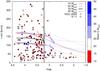 |
Fig. 1 Projected rotational velocity versus surface gravity for stars in the FLAMES survey near LMC clusters NGC 2004 (triangles) and N11 (circles). Color coding indicates the stellar mass. We use the sudden transition at log g = 3.2 (vertical line) to calibrate the amount of overshooting of our 16 M⊙ model (black line), see Sect. 2.4. For comparison we plot several other models with different initial masses and rotation rates (dotted lines). |
In an alternate scenario discussed by Vink et al. (2010), the population of slow rotators might be main-sequence stars, that have spun down due to increased mass loss (bi-stability breaking). However, this would require a huge overshooting, in order to extend the lifetime of main sequence stars at temperatures below the bi-stability temperature of about 22 kK. With the current overshooting calibration, bi-stability breaking plays a role only well above 30 M⊙. The nature of the evolved slow rotators in Fig. 1 remains puzzling. The fact that all of them have a strong nitrogen surface enhancement might propose that they are post-red supergiants which acquired the nitrogen enhancement through the first dredge-up (Vink et al. 2010), but they might as well be products of binary interaction or of so far unidentified physical processes.
For the overshooting calibration we use a stellar model with a mass and rotation rate that are representative for the entire sample. The typical mass is about 16 M⊙ (based on evolutionary masses; see Paper II) and the mean projected velocity of the stars in the sample with log g ≥ 3.2 dex is ⟨ 3sini ⟩ = 110 km s-1. This corresponds to an average rotational velocity of ⟨ v ⟩ = 142 km s-1 assuming a random orientation of the spin axes, i.e. ⟨ sini ⟩ = π/4. Throughout the main-sequence evolution the equatorial velocity is expected to be nearly constant due to the reduced effect of stellar winds in the low metallicity environment of the LMC and due to coupling of the expanding envelope to the contracting core. Therefore, we use the typical velocity as an estimate of the average initial rotational velocity.
The full black line in Fig. 1 shows a model with the typical mass and rotation rate. The overshooting parameter has been adjusted to α = 0.335, such that the end of the main sequence coincides with the drop in rotational velocities at log g = 3.2. Figure 1 demonstrates that the adopted amount of overshooting, derived for a 16 M⊙ star, appears to be valid for the mass range 10 to 20 M⊙. However, it is unconstrained outside this range, as for example the 30 M⊙ tracks in Fig. 1 have no observed counterparts near the TAMS. We therefore use an overshooting parameter of α = 0.335 for our entire grid. Given the uncertainty in the surface gravities (~0.15 dex), we estimate the uncertainty of the overshooting parameter in the mass range 10 to 20 M⊙ to be 0.1.
A priori we do not expect the overshooting parameter to depend on metallicity. To check this we show the projected rotational velocities against surface gravity for the SMC and Galactic sample of the FLAMES survey in Fig. 2. The drop in rotation rate occurs at the same surface gravity within the measurement errors. The Galactic sample shows a second feature around log g = 3.5 caused mainly by stars below 5 M⊙. Dufton et al. (2006) already described this stars as over-luminous for their age and a general disappointing agreement of the clusters HR-diagram with isochrones. When we vary the initial composition from SMC to the Galactic mixture, we find that the end of the main sequence for our 16 M⊙ model shifts from log g ~ 3.3 to 3.1, adopting the same value for the overshooting parameter. This shift is also within the measurement uncertainties. Therefore, adopting one fixed value for the overshooting parameter in our entire model grid is a reasonable assumption.
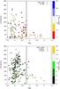 |
Fig. 2 Similar to Fig. 1, but now for the SMC (top) and Galactic (bottom) samples of the FLAMES survey. The typical error in log g is about 0.15 dex. The drop in rotation rate, which may be interpreted as the end of the main sequence, occurs around log g = 3.2 (vertical line) independently of metallicity. |
2.5. Calibration of the rotational mixing efficiency
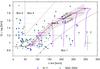 |
Fig. 3 Nitrogen surface abundance versus projected rotational velocity for stars in the LMC sample of the FLAMES survey (Hunter et al. 2009) in the N11 (blue) and the NGC 2004 (green) fields. Stars with evidence for a binary companion from radial velocity variations are plotted as triangles. Black solid lines indicate regions that are helpful as a reference in later discussion (see also Paper II). Evolutionary tracks of 13 M⊙ models are plotted for various rotational velocities, shifted by a factor π/4 to account for random inclination angles. The red line marks the nitrogen abundance reached at the end of the main sequence for 13 M⊙ models adopting a mixing efficiency of fc = 0.0228 (our calibration). Thin dotted lines show the location of the line, if different values for fc are adopted, e.g. fc = 0.015 (lower line) and fc = 0.03 (upper line). |
As mentioned in the beginning of Sect. 2 we treat all mixing processes as diffusive processes, where the diffusion coefficient is taken as the sum of the individual diffusion coefficients for the various mixing processes. The contributions of all rotationally induced mixing processes are reduced by a factor, fc, before they are added to the total diffusion coefficient for transport of chemicals. Pinsonneault et al. (1989) was the first to introduce this parameter. In order to explain the solar lithium abundance they needed to reduce the efficiency of rotationally induced mixing processes by a factor fc = 0.046. Based on theoretical considerations Chaboyer & Zahn (1992) proposed fc = 0.033, which was adopted in the models of Heger et al. (2000). We note that we cannot compare our efficiency parameter directly with these values due to differences in the implementation and the considered specific set of mixing and angular momentum transport processes.
We calibrate the mixing efficiency for our models using the B-stars in the LMC sample of the FLAMES survey. We aim to reproduce the main trend of the observed nitrogen surface abundances with the projected rotational velocity for the nitrogen enriched fast rotators. In Fig. 3 we present the data, indicating different regions or boxes which have been numbered for reference (Hunter et al. 2008a, and Paper II). The majority of the sample, about 53% of the stars, is not significantly enriched in nitrogen, given the typical error of 0.2 dex for the nitrogen abundance measurements. This group is indicated as Box 5 in Fig. 3. Fast rotators with significantly enhanced surface abundances (>7.2 dex; see Box 3) constitute 18% of the sample. A detailed discussion of the stars in Box 1 and 2, which deviate from the main trend, and of observational biases and other factors that might influence this numbers are provided in Paper II and Hunter et al. (2008a).
For the calibration we use stellar models with a mass that is typical for the stars for which we have nitrogen surface abundance measurements, i.e. 13 M⊙. We adjust the mixing efficiency such that the nitrogen surface abundances reached at the end of the main-sequence evolution follow the trend of the stars in Box 3 while we make sure that the slow rotators do not enrich more than 0.2 dex to match the stars in Box 5. We find that this is obtained for a mixing efficiency of fc = 0.0228. In Fig. 3 we plot evolutionary tracks for several 13 M⊙ models with different initial rotation rates. Adopting this mixing efficiency, a model with the typical mass and average rotational velocity (3ZAMS = 142 km s-1) reaches a surface nitrogen enhancement of 7.2 dex at the end of its main sequence. To illustrate the sensitivity of the nitrogen surface abundances to the adopted mixing efficiency, we depict the surface abundances reached at the end of the main sequence for fc = 0.015 and fc = 0.03 (dotted lines and grey band). As we have no reason to believe that the mixing efficiency fc depends on metallicity, we adopt the same value for the SMC and the Galactic grid.
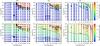 |
Fig. 4 Surface abundance of nitrogen (bottom row) and helium (top row) reached at the end of the main sequence (colors and contours) in our models with different initial masses, rotational velocities and compositions. Each evolutionary sequence of our grids is represented by one dot in this diagram. See Sect. 2.6 for a description of the initial parameter space of our grid and Sect. 4 for a discussion of the abundances. |
Description of the online tables containing the results of our evolutionary calculations as a function of time, for given initial composition, initial mass and initial rotation rate.
2.6. Grid of evolutionary tracks and isochrones: initial parameters and description of provided data
Using the calibration and the three initial compositional mixtures described above we computed a grid of evolutionary models. We adopt initial masses between 5 and 60 M⊙ and initial equatorial rotational velocities (3ZAMS) ranging from 0 to about 600 km s-1. For each initial composition we computed about 200 evolutionary tracks. The spacing between the initial parameters was chosen to provide a proper coverage of the parameter space and to provide extra resolution for massive fast rotating stars whose evolution depends sensitively on the initial rotation rate (see Fig. 4).
The results of our calculations are made available online through VizieR in table format. For each evolutionary track we provide the basic stellar parameters at different ages such as the mass, effective temperature, luminosity, radius and mass-loss rate as well as the surface abundances of various elements. We also list the central and surface mass fractions of the most important isotopes of these elements. In Table 3 we summarized all the provided data. The time steps are chosen to resolve the evolutionary changes of the main stellar parameters. Tracks with higher time resolution are available from the authors upon request.
Based on these evolutionary tracks we generated sets of isochrones, using our population synthesis code STARMAKER (Paper II). The isochrones cover the evolution until central hydrogen exhaustion for stellar masses between 5 and 60 M⊙. We provide them for ages between 0 and 35 Myr at intervals of 0.2 Myr, for initial rotational velocities between 0 and 540 km s-1 with steps of 10 km s-1 and for three different initial compositions: SMC, LMC and a Galactic mixture. We provide the basic stellar parameters and surface abundances as listed in Table 4.
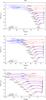 |
Fig. 5 Evolutionary tracks for various masses and metallicities. Red tracks are the non-rotating models and in blue we show models rotating initially at about 550 km s-1. For clarity, we alternate different line styles and scaled the temperature ranges such that the maximum of each plot is visible. |
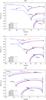 |
Fig. 6 Evolutionary tracks for 15, 25 and 50 M⊙ for SMC, LMC and Galactic composition (from top to bottom), for a range of initial rotational velocities (see legend). |
3. Evolutionary tracks and isochrones
3.1. Evolutionary tracks
Rotation affects evolutionary tracks in the Hertzsprung-Russell diagram (e.g. Maeder & Meynet 2000, and references therein). The centrifugal acceleration reduces the effective gravity resulting in cooler and slightly less luminous stars. However, rotation also induces internal mixing processes which can have the opposite effect, leading to more luminous and hotter stars. Which of these effects dominates depends on the initial mass, rotation rate, metallicity and the evolutionary stage. In this section we describe the effects of rotation on our models.
In rotating stars, the radiative energy flux depends on the local effective gravity (von Zeipel 1924), and temperature and luminosity become latitude dependent. The resulting thermal imbalance drives large scale meridional currents. In most stars, rotating at moderate rotation rates, the expected latitude dependence of temperature and luminosity is week (Hunter et al. 2009). In models close to critical rotation, luminosity and temperature differences are expected to be more significant and may even give rise to polar winds and equatorial outflows caused by critical rotation (Maeder 1999). Temperatures, luminosities and gravities given for the models presented in this paper are surface averaged values.
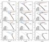 |
Fig. 7 Isochrones for SMC (left panels), LMC (center) and galaxy (right) composition. Each panel shows isochrones for a given age and initial rotational velocity ranging from 0 to 540 km s-1 in steps of 20 km s-1, with an increased resolution of 10 km s-1 between 350 and 450 km s-1 (grey lines). In red we show the isochrone for non rotating models, for other colors see the legend and the main text. We show the area spanned by the zero-age isochrones as a light blue band. The age in the second row has been chosen such that the isochrones span the largest range in effective temperature, 1 Myr earlier is shown in the first row, 1 and 5 Myr later are shown in the third and fourth row. |
Mass dependence of rotational mixing:
for intermediate mass main-sequence stars the main effect of rotation is a reduction of the effective gravity by centrifugal acceleration. Figure 5 shows that, during the main-sequence evolution, the tracks of the fast rotating 5 M⊙ stars are about 2000 K cooler compared to the nonrotating counterparts. Rotational mixing does affect the surface abundances of those elements that are so fragile that the relatively low temperatures in the stellar envelope are sufficient to induce nuclear reactions on them. However, the mixing is not efficient enough to significantly alter the structure of the star. As a consequence, the effect of rotation on the corresponding evolutionary tracks in the Hertzsprung-Russell diagram remains limited.
In rapid rotators more massive than about 15 M⊙, the effect of rotational mixing becomes more important than that of the reduced effective gravity: towards the cool edge of the main sequence band, the rotating stars become more luminous than the nonrotating ones. The main effect of rotation is an effective increase of the size of the stellar core, similar to the effect of overshooting (Sect. 2.4). This can be seen in Fig. 5 when one compares the tracks of the 15 and 16 M⊙ models near the end of their main-sequence evolution. The larger core mass in the fast rotating models results in a higher luminosity.
In the most massive stars at low metallicity (≳ 16 M⊙ for the SMC, M ≳ 19 M⊙ for the LMC), and for the extreme rotators shown in Fig. 5, mixing induced by rotation is so efficient that almost all the helium produced in the center is transported throughout the entire envelope of the star. During their main-sequence evolution they become brighter and hotter, evolving up- and bluewards in the Hertzsprung-Russell diagram. After all hydrogen in the center has been converted to helium, the star contracts, reaching effective temperatures of up to 100 000 K. This type of evolution is referred to as “quasi-chemically homogeneous evolution” (Maeder 1987; Yoon & Langer 2005; Woosley & Heger 2006). The blueward and redward evolution after the exhaustion of hydrogen in the center is analogous to the “hook” at the end of the main sequence seen in tracks of nonrotating stars. Note that all models have been computed beyond central hydrogen exhaustion, in most cases up to the ignition of helium. This allows us to later compare the main sequence surface abundances with those resulting from the first dredge-up in the red supergiant regime.
Metallicity dependence of rotational mixing:
Fig. 6 depicts evolutionary tracks of models with various initial rotation rates. The most striking feature in these diagrams is the bifurcation of the evolutionary tracks occurring at high masses and low metallicity, most clearly visible at SMC metallicity. Stars that rotate faster than a certain threshold are so efficiently mixed that they evolve almost chemically homogeneously. Stars that rotate slower than this threshold build a chemical gradient at the boundary between the convective core and the radiative envelope. This gradient itself has an inhibiting effect on the mixing processes, strongly reducing the transport of material from the core to the envelope. The minimum rotation rate required for chemically homogeneous evolution decreases with increasing mass (Yoon et al. 2006).
At high metallicity, rotational mixing is less efficient. In addition, mass and angular momentum loss due to stellar winds becomes important, slowing down the rotation rate and therefore the efficiency of the mixing processes. The fastest rotating stars at high metallicity initially evolve blue- and upward in the Hertzsprung-Russell diagram, see in the lower panel of Fig. 6. However, the combined effects of spin down by a stellar wind and the build up of an internal chemical gradient reduces the efficiency of internal mixing processes. The star switches onto a redward evolutionary track, similar to that of a non rotating star. However, its larger core mass results in a higher luminosity compared to the slower rotating counterparts.
3.2. Isochrones
While for a given metallicity, a classical isochrone can be represented by a single line in the Hertzsprung-Russell diagram, the isochrones of rotating stars span an area for a given age and initial composition. This is shown in Fig. 7. The isochrone constructed from nonrotating evolutionary models is plotted in red. The isochrone corresponding to the fastest initial rotational velocity for which the models do not yet follow a blueward evolution in the HRD is plotted in black. The isochrone with the slowest initial velocity that shows a clear bluewards evolution is shown in green. In blue and yellow we have selected two isochrones from the transition region that may help the reader to asses the sudden transition from classical to chemically homogeneous evolution.
For rotational velocities above 350 km s-1, when the most massive stars undergo chemically homogeneous evolution, the isochrones deviate strongly from the nonrotating case. The maximum spread in effective temperature occurs around 4 Myr (second row in Fig. 7). At lower metallicity the isochrones split into more clearly separated branches. At SMC metallicity (e.g. the third panel in the first column in Fig. 7) the isochrone based on models rotating initially at 500 km s-1 moves straight to the blue. In contrast, the comparable LMC isochrone returns to the red for stars above ~ 50 M⊙. This behavior is directly related to the feature in the evolutionary LMC tracks in Fig. 6, see for example the 50 M⊙ track for 550 km s-1. At Galactic metallicity the blueward evolution does not appear in the models. Nevertheless, the area spanned by the isochrones extends over a wide range of effective temperatures.
Between about 5 and 10 Myr the most massive nonrotating stars have evolved off the main sequence. However, at low metallicity, the most massive fast rotators, which undergo chemically homogeneous evolution are still in their main-sequence phase at this time, forming a blue straggler-like blue population (see the bottom panels of Figs. 7). If homogeneously evolving stars exist in nature they would most likely be found in low metallicity star clusters with ages between 5 and 10 Myr.
4. Surface abundances
4.1. Abundances as a function of time
A direct observable consequence of rotationally induced mixing is the enrichment or depletion of certain elements in the atmospheres of main-sequence stars. In Figs. 9 − 11 we show the evolution of the surface abundance of various elements as a function time. The effects of rotational mixing are more pronounced at lower metallicity, at higher masses and for higher rotational velocity (see also Fig. 4 and Sect. 3).
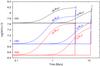 |
Fig. 8 Nitrogen as a function of time at SMC, LMC and Galactic metallicity. The models are of 15 and 40 M⊙. Full lines represent nonrotating models, dashed lines models rotating initially at ~ 270 km s-1. |
As is usual in observational work, we express the surface abundances relative to the abundance of hydrogen. When stars become significantly hydrogen depleted at the surface, using hydrogen as a reference element may not be the most logical choice. Changes in the abundance may partially reflect changes in the reference element hydrogen. We plot the abundances in red when these effects become important (i.e. when the helium mass fraction at the surface becomes larger than 40%).
Most of our stellar models evolve to the red supergiant stage directly after the end of core hydrogen burning. This leads to a large vertical step in the surface abundances of many elements in Figs. 9 − 11, which is due to the convective dredge-up in the red supergiant stage. In the following, we discuss the evolution of the surface abundances of various groups of elements, focusing on the changes occurring over the course of the main-sequence evolution.
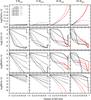 |
Fig. 9 Change of the surface abundances of helium, lithium, beryllium and boron along evolutionary tracks of SMC composition as a function of time, expressed as a fraction of the main-sequence lifetime. Different line styles represent different initial rotational velocities (see legend). For models where the surface helium mass fraction exceeded 40%, the abundances are plotted in red, to indicate that the reference element hydrogen is depleted significantly (see also Sect. 4). |
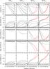 |
Fig. 9 continued. Surface abundances of rotating models at SMC metallicity, continued. Shown are carbon, oxygen, nitrogen, fluorine and sodium (from top to bottom) as a function of time, expressed as a fraction of the main-sequence lifetime. |
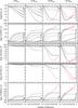 |
Fig. 10 continued. |
4.1.1. Helium
Even though helium is the main product of hydrogen burning, the abundance of helium at the surface remains remarkably constant in most evolutionary tracks during the main-sequence phase. For the 12 M⊙ models the enhancement is less than 0.2 dex. Only the fast rotators of 30 and 60 M⊙ show significant helium surface enrichments, especially at low metallicity (Figs. 9 − 11). These behaviors can be understood as the combination of two effects. Firstly, the production of helium occurs on the nuclear timescale. This occurs slower than, for example, the production of nitrogen or destruction of Li. Secondly, with the production of helium a steep gradient in mean molecular weight is established at the boundary between the core and the envelope. Such gradients inhibit the efficiency of mixing processes and prevent the transport of helium to the surface. Significant amounts of helium can be transported to the surface in models were mixing processes are efficient enough to prevent the build-up of a chemical barrier between core and envelope.
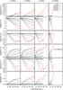 |
Fig. 12 Surface abundances for a fixed age, as a function of initial mass and rotational velocity, for SMC metallicity. From top to bottom are shown helium, boron, carbon, nitrogen, oxygen and sodium abundances. |
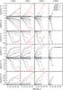 |
Fig. 13 Surface abundances for a fixed age, as a function of initial mass and rotational velocity, for LMC metallicity. From top to bottom are shown helium, boron, carbon, nitrogen, oxygen and sodium abundances. |
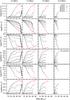 |
Fig. 14 Surface abundances for a fixed age, as a function of initial mass and rotational velocity, for Galactic metallicity. From top to bottom are shown helium, boron, carbon, nitrogen, oxygen and sodium abundances. |
4.1.2. The fragile elements, Li, Be, B and F
The elements Li, Be, B are destroyed by proton captures at temperatures higher than 2.5 × 10⁶ K for lithium, 3.5 × 10⁶ K for beryllium, 5 × 10⁶ K for boron (McWilliam & Rauch 2004, p. 123). These elements can only survive in the outermost layers. In rotating stars the surface abundances of these elements decrease gradually as the outer layers are mixed with deeper layers in which these elements have been destroyed. The decrease is most rapid for the most fragile element, lithium. The surface abundance of fluorine behaves similarly. It can survive temperatures of up to about 20 × 106 K. We note that the rates of the reactions in which fluorine is involved are quite uncertain (Arnould et al. 1999).
In addition, stellar winds can affect the surface abundances especially for the most massive stars at high metallicity. Due to mass loss deeper layers are revealed in which the fragile elements have been destroyed. For nonrotating stars a sudden drop in the surface abundances of the fragile elements is visible in Figs. 9 − 11, when mass loss has removed the layers in which these elements can survive. In rotating models the change is more gradual.
After the end of the main-sequence, dredge-up leads to a further decrease of the surface abundances of these elements. However, for some models with masses between 20 and 40 M⊙ we find that small amounts of Li and Be are produced in the hydrogen burning shell by the p-p chain. As a result of the interplay between a convective zone on top of the shell source and the convective envelope reaching into these layers after hydrogen exhaustion, we find that the surface abundances of these elements can be significantly increased in these models. Even though the possible production of these elements by massive stars has several interesting applications, the robustness of the predictions for these elements requires further investigation.
4.1.3. Carbon, nitrogen, oxygen and sodium
Carbon, nitrogen and oxygen take part as catalysts in the conversion of hydrogen into helium. Although their sum remains roughly constant, nitrogen is produced when the cycle settles into equilibrium, at the expense of carbon and, somewhat later, oxygen. The CN-equilibrium is achieved very early in the evolution, before a strong mean molecular weight gradient has been established between the core and the envelope. Therefore, rotational mixing can transport nitrogen throughout the envelope to the stellar surface. While the surface abundance of nitrogen increases, carbon is depleted. Since full CNO-equilibrium is achieved only after a significant amount of hydrogen has been burnt in the core, changes in the oxygen surface abundance are only found in later stages in the more massive and faster rotating models.
Sodium is produced in the extension of the CNO-cycle, the NeNa-chain. The changes in the surface abundances of sodium resemble the changes is nitrogen, even though the enhancements are smaller and appear a little bit later at the stellar surface, see Figs. 9 − 11.
The relative increase of the nitrogen abundance depends on the initial amount of carbon available for conversion into nitrogen. These amounts are different for the different mixtures. The C/N ratio in the SMC and LMC composition are similar (7.4 and 7.1, respectively), while the ratio in our Galactic composition is smaller (3.1). In Fig. 8 we show the evolution of the surface nitrogen abundance in models of 15 and 40 M⊙ with initial rotation rates of 0 and 270 km s-1 for SMC, LMC and Galactic composition. The initial abundance of nitrogen in the Magellanic clouds is much lower than in the Galactic mixture. Nevertheless, the rotating SMC and LMC models reach surface nitrogen abundances at the TAMS which can be higher than in the initial Galactic mixture. The steep rise at the end of the curves is due to the dredge-up when the star becomes a red supergiant. The TAMS is located at the base of the steep rise.
4.2. Surface abundances for selected ages
Due to the effects of rotation, the age or mass of a star can no longer be determined uniquely from its position in the Hertzsprung-Russell diagram by fitting evolutionary tracks or isochrones. This holds especially for stars that are located near the zero-age main sequence. A young, unevolved, slowly rotating star may have the same effective temperature and luminosity as a less massive, fast rotating, evolved star. A determination of the surface composition and to some extent the projected rotational velocity may help to lift this degeneracy.
In the panels of Figs. 12–14 we show which abundance distributions are predicted at a given time, as function of the considered mass and rotational velocity. Models of more massive stars show more pronounced surfaces abundances changes for a given age. The kinks in the lines of 400 km s-1 at LMC and Galactic composition occur due to difficulties in the interpolation between stars that follow blueward and redward evolutionary tracks effects.
These plots also show the effect of rotation on the main sequence life time. For example, Fig. 14 shows that the lines representing models with initial rotation rates of 400 and 500 km s-1 predict that stars of 50 and 60 M⊙ are still present at 4 Myr, whereas nonrotating models predict that they have left the main sequence. On a much smaller scale this effect is also visible if one compares lines for rotation rates between 0 and 300 km s-1 based on models that follow normal evolutionary tracks.
The steep drop in the boron abundance along the isochrones based on nonrotating models is related to the stellar wind mass loss. For example, at LMC composition, the drop occurs around 35 M⊙, indicating that the winds efficiently remove the outer layers of stars of 35 M⊙ and higher (see also Sect. 4.1.2).
5. Summary
In this paper we have presented an extensive grid of models for rotating massive main sequence stars. We provide three sets of initial compositions that are suitable for comparison with early OB stars in the SMC, the LMC and the Galaxy. The models cover the main-sequence evolution and in most cases these have been computed up to helium ignition. In terms of overshooting and rotational mixing efficiency, our models have been calibrated against the FLAMES survey of massive stars. We are using a new method to calibrate the amount of overshooting that makes use of the observed drop in projected rotation rates for stars with surface gravities lower than log g = 3.2 dex. Interpreting this drop as the end of the main sequence, we find an overshooting parameter of 0.34 ± 0.1 pressure scale heights.
We have also presented a detailed set of isochrones based on models of rotating massive main sequence stars. Whereas classical isochrones can be represented by a single line in the Hertzsprung-Russell diagram, the isochrones of rotating stars span a wide range of effective temperatures at a given luminosity. Therefore, the mass and age of an observed star can no longer be determined uniquely from its location in the Hertzsprung-Russell diagram. We also provided detailed predictions for the changing surface abundances of rotating massive main sequence stars. While we believe that the data provided here can be useful to many future studies of massive stars, we make use of it in Paper II for undertaking a quantitative test of rotational mixing of massive stars in the LMC.
Acknowledgments
We thank Georges Meynet, the referee of this paper, for many helpful comments and suggestions. This work has been performed within the framework of the FLAMES consortium of massive stars and has made use of the VizieR catalogue access tool, CDS, Strasbourg, France. S.d.M. acknowledges support for this work provided by NASA through Hubble Fellowship grant HST-HF-51270.01-A awarded by the Space Telescope Science Institute, which is operated by the Association of Universities for Research in Astronomy, Inc., for NASA, under contract NAS 5-26555.
References
- Arnould, M., Goriely, S., & Jorissen, A. 1999, A&A, 347, 572 [NASA ADS] [Google Scholar]
- Asplund, M., Grevesse, N., & Sauval, A. J. 2005, in Cosmic Abundances as Records of Stellar Evolution and Nucleosynthesis, ed. T. G. Barnes III, & F. N. Bash, ASP Conf. Ser., 336, 25 [Google Scholar]
- Böhm-Vitense, E. 1958, ZAp, 46, 108 [NASA ADS] [Google Scholar]
- Braithwaite, J. 2006, A&A, 449, 451 [NASA ADS] [CrossRef] [EDP Sciences] [Google Scholar]
- Briquet, M., Morel, T., Thoul, A., et al. 2007, MNRAS, 381, 1482 [NASA ADS] [CrossRef] [Google Scholar]
- Brott, I., Hunter, I., Anders, P., & Langer, N. 2008, in First Stars III, ed. B. W. O’Shea &, & A. Heger, AIP Conf. Ser., 990, 273 [Google Scholar]
- Brott, I., Evans, C. J., Hunter, I., et al. 2011, A&A 530, A116 [Google Scholar]
- Chaboyer, B., & Zahn, J.-P. 1992, A&A, 253, 173 [NASA ADS] [Google Scholar]
- Chiosi, C., & Maeder, A. 1986, ARA&A, 24, 329 [NASA ADS] [CrossRef] [Google Scholar]
- Claret, A. 2007, A&A, 475, 1019 [NASA ADS] [CrossRef] [EDP Sciences] [Google Scholar]
- de Koter, A., Heap, S. R., & Hubeny, I. 1997, ApJ, 477, 792 [Google Scholar]
- Douglas, L. S., Bremer, M. N., Stanway, E. R., Lehnert, M. D., & Clowe, D. 2009, MNRAS, 400, 561 [NASA ADS] [CrossRef] [Google Scholar]
- Dufton, P. L., Smartt, S. J., Lee, J. K., et al. 2006, A&A, 457, 265 [NASA ADS] [CrossRef] [EDP Sciences] [Google Scholar]
- Endal, A. S., & Sofia, S. 1976, ApJ, 210, 184 [NASA ADS] [CrossRef] [Google Scholar]
- Endal, A. S., & Sofia, S. 1978, ApJ, 220, 279 [NASA ADS] [CrossRef] [Google Scholar]
- Evans, C. J., Smartt, S. J., Lee, J.-K., et al. 2005, A&A, 437, 467 [NASA ADS] [CrossRef] [EDP Sciences] [Google Scholar]
- Evans, C. J., Lennon, D. J., Smartt, S. J., & Trundle, C. 2006, A&A, 456, 623 [NASA ADS] [CrossRef] [EDP Sciences] [Google Scholar]
- Fitzpatrick, E. L., & Garmany, C. D. 1990, ApJ, 363, 119 [NASA ADS] [CrossRef] [Google Scholar]
- Georgy, C., Meynet, G., Walder, R., Folini, D., & Maeder, A. 2009, A&A, 502, 611 [NASA ADS] [CrossRef] [EDP Sciences] [Google Scholar]
- González, J. F., Ostrov, P., Morrell, N., & Minniti, D. 2005, ApJ, 624, 946 [NASA ADS] [CrossRef] [Google Scholar]
- Grevesse, N., Noels, A., & Sauval, A. J. 1996, in Cosmic Abundances, ed. S. S. Holt, & G. Sonneborn, ASP Conf. Ser., 99, 117 [Google Scholar]
- Haiman, Z., & Loeb, A. 1997, ApJ, 483, 21 [NASA ADS] [CrossRef] [Google Scholar]
- Hamann, W., Koesterke, L., & Wessolowski, U. 1995, A&A, 299, 151 [NASA ADS] [Google Scholar]
- Heger, A., Langer, N., & Woosley, S. E. 2000, ApJ, 528, 368 [NASA ADS] [CrossRef] [Google Scholar]
- Heger, A., Woosley, S. E., & Spruit, H. C. 2005, ApJ, 626, 350 [NASA ADS] [CrossRef] [Google Scholar]
- Hunter, I., Dufton, P. L., Smartt, S. J., et al. 2007, A&A, 466, 277 [NASA ADS] [CrossRef] [EDP Sciences] [Google Scholar]
- Hunter, I., Brott, I., Lennon, D. J., et al. 2008a, ApJ, 676, L29 [NASA ADS] [CrossRef] [Google Scholar]
- Hunter, I., Lennon, D. J., Dufton, P. L., et al. 2008b, A&A, 479, 541 [NASA ADS] [CrossRef] [EDP Sciences] [Google Scholar]
- Hunter, I., Brott, I., Langer, N., et al. 2009, A&A, 496, 841 [NASA ADS] [CrossRef] [EDP Sciences] [Google Scholar]
- Iglesias, C. A., & Rogers, F. J. 1996, ApJ, 464, 943 [NASA ADS] [CrossRef] [Google Scholar]
- Kippenhahn, R., & Thomas, H. 1970, in Stellar Rotation, IAU Colloq., 4, 20 [Google Scholar]
- Kudritzki, R. P., Urbaneja, M. A., Bresolin, F., & Przybilla, N. 2008, Phys. Scr. T, 133, 014039 [NASA ADS] [CrossRef] [Google Scholar]
- Kurt, C. M., & Dufour, R. J. 1998, in Rev. Mex. Astron. Astrofis. Conf. Ser. 7, ed. R. J. Dufour, & S. Torres-Peimbert, 202 [Google Scholar]
- Langer, N. 1991, A&A, 252, 669 [NASA ADS] [Google Scholar]
- Langer, N., Fricke, K. J., & Sugimoto, D. 1983, A&A, 126, 207 [NASA ADS] [Google Scholar]
- Langer, N., El Eid, M. F., & Fricke, K. J. 1985, A&A, 145, 179 [NASA ADS] [Google Scholar]
- Maeder, A. 1987, A&A, 178, 159 [NASA ADS] [Google Scholar]
- Maeder, A. 1999, A&A, 347, 185 [NASA ADS] [Google Scholar]
- Maeder, A. 2000, New Astron. Rev., 44, 291 [NASA ADS] [CrossRef] [Google Scholar]
- Maeder, A., & Meynet, G. 1987, A&A, 182, 243 [NASA ADS] [Google Scholar]
- Maeder, A., & Meynet, G. 2000, ARA&A, 38, 143 [NASA ADS] [CrossRef] [Google Scholar]
- Maeder, A., & Meynet, G. 2005, A&A, 440, 1041 [NASA ADS] [CrossRef] [EDP Sciences] [Google Scholar]
- McWilliam, A., & Rauch, M. (ed.) 2004, Origin and Evolution of the Elements, Carnegie Obs. Astrophys. Ser. (CUP) [Google Scholar]
- Mermilliod, J., & Maeder, A. 1986, A&A, 158, 45 [NASA ADS] [Google Scholar]
- Meynet, G., & Maeder, A. 1997, A&A, 321, 465 [NASA ADS] [Google Scholar]
- Meynet, G., & Maeder, A. 2000, A&A, 361, 101 [NASA ADS] [Google Scholar]
- Meynet, G., & Maeder, A. 2005, A&A, 429, 581 [Google Scholar]
- Mitalas, R., & Falk, H. J. 1984, MNRAS, 210, 641 [NASA ADS] [Google Scholar]
- Napiwotzki, R., Schoenberner, D., & Weidemann, V. 1991, A&A, 243, L5 [NASA ADS] [Google Scholar]
- Nieuwenhuijzen, H., & de Jager, C. 1990, A&A, 231, 134 [NASA ADS] [Google Scholar]
- Ohkubo, T., Nomoto, K., Umeda, H., Yoshida, N., & Tsuruta, S. 2009, ApJ, 706, 1184 [NASA ADS] [CrossRef] [Google Scholar]
- Peimbert, M., Luridiana, V., & Peimbert, A. 2007, ApJ, 666, 636 [NASA ADS] [CrossRef] [Google Scholar]
- Petrovic, J., Langer, N., Yoon, S., & Heger, A. 2005, A&A, 435, 247 [NASA ADS] [CrossRef] [EDP Sciences] [Google Scholar]
- Pinsonneault, M. H., Kawaler, S. D., Sofia, S., & Demarque, P. 1989, ApJ, 338, 424 [NASA ADS] [CrossRef] [Google Scholar]
- Przybilla, N., Nieva, M., & Butler, K. 2008, ApJ, 688, L103 [NASA ADS] [CrossRef] [Google Scholar]
- Ribas, I., Jordi, C., & Giménez, Á. 2000, MNRAS, 318, L55 [NASA ADS] [CrossRef] [Google Scholar]
- Savaglio, S. 2006, New J. Phys., 8, 195 [NASA ADS] [CrossRef] [Google Scholar]
- Schröder, K., Pols, O. R., & Eggleton, P. P. 1997, MNRAS, 285, 696 [NASA ADS] [CrossRef] [Google Scholar]
- Spruit, H. C. 2002, A&A, 381, 923 [NASA ADS] [CrossRef] [EDP Sciences] [Google Scholar]
- Spruit, H. C. 2006, [arXiv:astro-ph/0607164] [Google Scholar]
- Suijs, M. P. L., Langer, N., Poelarends, A., et al. 2008, A&A, 481, L87 [NASA ADS] [CrossRef] [EDP Sciences] [Google Scholar]
- Tassoul, J. 1978, Theory of rotating stars (Princeton: University Press) [Google Scholar]
- Trundle, C., Dufton, P. L., Hunter, I., et al. 2007, A&A, 471, 625 [NASA ADS] [CrossRef] [EDP Sciences] [Google Scholar]
- Venn, K. A. 1995, ApJS, 99, 659 [NASA ADS] [CrossRef] [Google Scholar]
- Venn, K. A. 1999, ApJ, 518, 405 [NASA ADS] [CrossRef] [Google Scholar]
- Vink, J. S., de Koter, A., & Lamers, H. J. G. L. M. 2000, A&A, 362, 295 [NASA ADS] [Google Scholar]
- Vink, J. S., de Koter, A., & Lamers, H. J. G. L. M. 2001, A&A, 369, 574 [NASA ADS] [CrossRef] [EDP Sciences] [Google Scholar]
- Vink, J. S., Brott, I., Gräfener, G., et al. 2010, A&A, 512, L7 [NASA ADS] [CrossRef] [EDP Sciences] [Google Scholar]
- von Zeipel, H. 1924, MNRAS, 84, 665 [NASA ADS] [CrossRef] [Google Scholar]
- Woosley, S. E., & Heger, A. 2006, ApJ, 637, 914 [NASA ADS] [CrossRef] [Google Scholar]
- Yoon, S., & Langer, N. 2005, A&A, 443, 643 [NASA ADS] [CrossRef] [EDP Sciences] [Google Scholar]
- Yoon, S.-C., Langer, N., & Norman, C. 2006, A&A, 460, 199 [NASA ADS] [CrossRef] [EDP Sciences] [Google Scholar]
- Zahn, J. 1992, A&A, 265, 115 [NASA ADS] [Google Scholar]
- Zahn, J., Brun, A. S., & Mathis, S. 2007, A&A, 474, 145 [NASA ADS] [CrossRef] [EDP Sciences] [Google Scholar]
All Tables
Resulting hydrogen (X), helium (Y) and metal (Z) mass fractions for the chemical mixtures used in our models.
Description of the online tables containing the results of our evolutionary calculations as a function of time, for given initial composition, initial mass and initial rotation rate.
All Figures
|
Fig. 1 Projected rotational velocity versus surface gravity for stars in the FLAMES survey near LMC clusters NGC 2004 (triangles) and N11 (circles). Color coding indicates the stellar mass. We use the sudden transition at log g = 3.2 (vertical line) to calibrate the amount of overshooting of our 16 M⊙ model (black line), see Sect. 2.4. For comparison we plot several other models with different initial masses and rotation rates (dotted lines). |
| In the text | |
|
Fig. 2 Similar to Fig. 1, but now for the SMC (top) and Galactic (bottom) samples of the FLAMES survey. The typical error in log g is about 0.15 dex. The drop in rotation rate, which may be interpreted as the end of the main sequence, occurs around log g = 3.2 (vertical line) independently of metallicity. |
| In the text | |
|
Fig. 3 Nitrogen surface abundance versus projected rotational velocity for stars in the LMC sample of the FLAMES survey (Hunter et al. 2009) in the N11 (blue) and the NGC 2004 (green) fields. Stars with evidence for a binary companion from radial velocity variations are plotted as triangles. Black solid lines indicate regions that are helpful as a reference in later discussion (see also Paper II). Evolutionary tracks of 13 M⊙ models are plotted for various rotational velocities, shifted by a factor π/4 to account for random inclination angles. The red line marks the nitrogen abundance reached at the end of the main sequence for 13 M⊙ models adopting a mixing efficiency of fc = 0.0228 (our calibration). Thin dotted lines show the location of the line, if different values for fc are adopted, e.g. fc = 0.015 (lower line) and fc = 0.03 (upper line). |
| In the text | |
|
Fig. 4 Surface abundance of nitrogen (bottom row) and helium (top row) reached at the end of the main sequence (colors and contours) in our models with different initial masses, rotational velocities and compositions. Each evolutionary sequence of our grids is represented by one dot in this diagram. See Sect. 2.6 for a description of the initial parameter space of our grid and Sect. 4 for a discussion of the abundances. |
| In the text | |
|
Fig. 5 Evolutionary tracks for various masses and metallicities. Red tracks are the non-rotating models and in blue we show models rotating initially at about 550 km s-1. For clarity, we alternate different line styles and scaled the temperature ranges such that the maximum of each plot is visible. |
| In the text | |
|
Fig. 6 Evolutionary tracks for 15, 25 and 50 M⊙ for SMC, LMC and Galactic composition (from top to bottom), for a range of initial rotational velocities (see legend). |
| In the text | |
|
Fig. 7 Isochrones for SMC (left panels), LMC (center) and galaxy (right) composition. Each panel shows isochrones for a given age and initial rotational velocity ranging from 0 to 540 km s-1 in steps of 20 km s-1, with an increased resolution of 10 km s-1 between 350 and 450 km s-1 (grey lines). In red we show the isochrone for non rotating models, for other colors see the legend and the main text. We show the area spanned by the zero-age isochrones as a light blue band. The age in the second row has been chosen such that the isochrones span the largest range in effective temperature, 1 Myr earlier is shown in the first row, 1 and 5 Myr later are shown in the third and fourth row. |
| In the text | |
|
Fig. 8 Nitrogen as a function of time at SMC, LMC and Galactic metallicity. The models are of 15 and 40 M⊙. Full lines represent nonrotating models, dashed lines models rotating initially at ~ 270 km s-1. |
| In the text | |
|
Fig. 9 Change of the surface abundances of helium, lithium, beryllium and boron along evolutionary tracks of SMC composition as a function of time, expressed as a fraction of the main-sequence lifetime. Different line styles represent different initial rotational velocities (see legend). For models where the surface helium mass fraction exceeded 40%, the abundances are plotted in red, to indicate that the reference element hydrogen is depleted significantly (see also Sect. 4). |
| In the text | |
|
Fig. 9 continued. Surface abundances of rotating models at SMC metallicity, continued. Shown are carbon, oxygen, nitrogen, fluorine and sodium (from top to bottom) as a function of time, expressed as a fraction of the main-sequence lifetime. |
| In the text | |
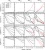 |
Fig. 10 Like Fig. 9, for stellar models of LMC composition. |
| In the text | |
|
Fig. 10 continued. |
| In the text | |
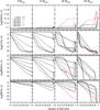 |
Fig. 11 Like Fig. 9 for stellar models with a Galactic initial composition. |
| In the text | |
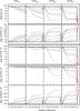 |
Fig. 11 continued. Like Fig. 9, for stellar models of Galactic composition. |
| In the text | |
|
Fig. 12 Surface abundances for a fixed age, as a function of initial mass and rotational velocity, for SMC metallicity. From top to bottom are shown helium, boron, carbon, nitrogen, oxygen and sodium abundances. |
| In the text | |
|
Fig. 13 Surface abundances for a fixed age, as a function of initial mass and rotational velocity, for LMC metallicity. From top to bottom are shown helium, boron, carbon, nitrogen, oxygen and sodium abundances. |
| In the text | |
|
Fig. 14 Surface abundances for a fixed age, as a function of initial mass and rotational velocity, for Galactic metallicity. From top to bottom are shown helium, boron, carbon, nitrogen, oxygen and sodium abundances. |
| In the text | |
Current usage metrics show cumulative count of Article Views (full-text article views including HTML views, PDF and ePub downloads, according to the available data) and Abstracts Views on Vision4Press platform.
Data correspond to usage on the plateform after 2015. The current usage metrics is available 48-96 hours after online publication and is updated daily on week days.
Initial download of the metrics may take a while.