| Issue |
A&A
Volume 529, May 2011
|
|
|---|---|---|
| Article Number | L4 | |
| Number of page(s) | 6 | |
| Section | Letters | |
| DOI | https://doi.org/10.1051/0004-6361/201116723 | |
| Published online | 08 April 2011 | |
Letters to the Editor
The reddening law of type Ia supernovae: separating intrinsic variability from dust using equivalent widths⋆
1
Université de Lyon, Université Lyon 1, CNRS/IN2P3, Institut de Physique Nucléaire de Lyon, 69622 Villeurbanne, France
e-mail: This email address is being protected from spambots. You need JavaScript enabled to view it.
2
Physics Division, Lawrence Berkeley National Laboratory, 1 Cyclotron Road, Berkeley, CA 94720, USA
3
LPNHE, Université Pierre et Marie Curie Paris 6, Université Paris Diderot Paris 7, CNRS-IN2P3, 75252 Paris Cedex 05, France
4
Department of Physics, Yale University, New Haven, CT 06250-8121, USA
5
Physikalisches Institut Universitat Bonn, Nussallee 12 53115 Bonn, Germany
6
Department of Physics, University of California Berkeley, 366 LeConte Hall MC 7300, Berkeley, CA, 94720-7300, USA
7
Computational Cosmology Center, Lawrence Berkeley National Laboratory, 1 Cyclotron Road, Berkeley, CA 94720, USA
8
Department of Astronomy, University of California, Berkeley, CA 94720-3411, USA
9
Observatoire de Lyon, 69230 Saint-Genis Laval, Université de Lyon, Université Lyon 1, 69003 Lyon, France
10
Australian National University, Mt. Stromlo Observatory, The RSAA, Weston Creek, ACT 2611, Australia
11
Centre de Physique des Particules de Marseille, 163 avenue de Luminy, Case 902, 13288 Marseille Cedex 09, France
12
Tsinghua Center for Astrophysics, Tsinghua University, Beijing 100084, PR China
13
New York University, Center for Cosmology and Particle Physics, 4 Washington Place, New York, NY 10003, USA
14
National Astronomical Observatories, Chinese Academy of Sciences, Beijing 100012, PR China
Received: 15 February 2011
Accepted: 28 March 2011
Abstract
We employ 76 type Ia supernovae (SNe Ia) with optical spectrophotometry within 2.5 days of B-band maximum light obtained by the Nearby Supernova Factory to derive the impact of Si and Ca features on the supernovae intrinsic luminosity and determine a dust reddening law. We use the equivalent width of Si ii λ4131 in place of the light curve stretch to account for first-order intrinsic luminosity variability. The resulting empirical spectral reddening law exhibits strong features that are associated with Ca ii and Si ii λ6355. After applying a correction based on the Ca ii H&K equivalent width we find a reddening law consistent with a Cardelli extinction law. Using the same input data, we compare this result to synthetic rest-frame UBVRI-like photometry to mimic literature observations. After corrections for signatures correlated with Si ii λ4131 and Ca ii H&K equivalent widths and introducing an empirical correlation between colors, we determine the dust component in each band. We find a value of the total-to-selective extinction ratio, RV = 2.8 ± 0.3. This agrees with the Milky Way value, in contrast to the low RV values found in most previous analyses. This result suggests that the long-standing controversy in interpreting SN Ia colors and their compatibility with a classical extinction law, which is critical to their use as cosmological probes, can be explained by the treatment of the dispersion in colors, and by the variability of features apparent in SN Ia spectra.
Key words: supernovae:general / dust, extinction / cosmology: observations
Table 1 is available in electronic form at http://www.aanda.org
© ESO, 2011
1. Introduction
Type Ia supernovae (SNe Ia) luminosity distances are measured via the standardization of their light curves using brightness-width (stretch, x1, Δm15) and color corrections (Phillips 1993; Tripp 1998; Guy et al. 2007; Jha et al. 2007). While the determination of the intrinsic dispersion related to the light curve shape is subject to small differences between fitters, the manner in which color is linked to dust is still controversial, because it may be affected by additional yet unidentified intrinsic dispersion. Whereas earlier work used the total-to-selective extinction ratio of the Milky Way, RV = 3.1, direct estimates from the supernovae (SNe) Hubble diagram fits lead to lower values, from RV = 1.7 to RV = 2.5 (Hicken et al. 2009; Tripp 1998; Wang et al. 2009). While the derivation of this value is subject to assumptions about the natural color dispersion of SNe (Freedman et al. 2009; Guy et al. 2010), the reason for a difference between SNe data and the Milky Way average result have remained unknown.
Equivalent widths are good spectral indicators for addressing this question because they probe the intrinsic variability of SNe Ia and by construction little depend on extinction owing to their narrow wavelength baseline. Arsenijevic et al. (2008) showed a strong correlation between the equivalent width of the Si ii λ4131 feature and the SALT2 x1 width parameter (Guy et al. 2007), and Bronder et al. (2008) showed its correlation with MB. Walker et al. (2011) used it to standardize the Hubble diagram, but were hindered from drawing firm conclusions by the quality of the low redshift data.
In this work, we take advantage of the Nearby Supernova Factory (SNfactory) spectrophotometric sample to revisit these conclusions, using both spectral data and derived UBVRI-like synthetic photometry. We present in Sect. 2 the SNe Ia sample and the definition of the Si ii λ4131 and Ca ii H&K equivalent widths, which will be used in Sect. 3.1 to correct the Hubble residuals. These corrected magnitudes are used to derive the relative absorption in each wavelength band, δAλ. The correlations between the δAλ from SN to SN across different bands provide the reddening law, as described in Sect. 3.2, as well as the dispersion matrix between bands. In Sect. 4 we show that the resulting reddening law agrees with a Cardelli extinction law (CCM, Cardelli et al. 1989; O’Donnell 1994). Our reddening law has a value of RV which agrees with the Milky-Way value of 3.1, when the proper dispersion matrix is used. We then discuss these results in Sect. 5 and conclude in Sect. 6.
2. Data set and derived quantities
This analysis uses flux calibrated spectra of 76 SNe Ia obtained by the SNfactory collaboration with its SNIFS instrument (Aldering et al. 2002) on the University of Hawaii 2.2-m telescope on Mauna Kea. This subset is selected in the same way as in Bailey et al. (2009), using only SNe with a measured spectrum within 2.5 days of B-band maximum, but with an enlarged data set with a redshift range of 0.007 < z < 0.09. The SALT2 x1 and c parameters (Fig. 1) and the spectra phases with respect to the B-band maximum light are derived using fits of the full light curves in three observer-frame top hat bandpasses corresponding approximately to BVR.
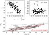 |
Fig. 1 Correlations of ewSi, SALT2 x1 (top left) and c (top right) parameters and measured peak absolute magnitude up to a constant term, δMB (bottom). The open circles in the bottom panel are the data points excluded from the fit, which is displayed as a solid line. |

After flux calibration, host galaxy subtraction, and correction for Milky Way extinction, the 76 spectra are transformed into rest frame. For the spectral analysis, they are rebinned with a resolution of 1500 km s-1. In addition, synthetic magnitudes are derived from the spectra after photon integration in a set of five UBVRI-like top-hat bandpasses with a constant resolution over the whole spectral range (3276 − 8635 Å, see Fig. 3 and caption). The uncorrected Hubble residuals δM(λ) = M(λ) − ⟨ M(λ) ⟩ are independently computed for each band of mean wavelength λ, relative to a flat ΛCDM universe with ΩM = 0.28 and H0 = 70 km s-1 Mpc-1. For the spectral analysis, the Hubble residuals are corrected for phase dependence using linear interpolation. For broad bands, we instead interpolate the magnitudes to the date of the B-maximum, using the light curve shape of each SN Ia as defined by the SALT2 x1 parameter, but with each band’s peak magnitude fitted separately. The data are presented in Table 1. The errors on Hubble residuals include statistical, calibration (~2% for peak luminosity), and redshift uncertainties. They are correlated between bands with a correlation coefficient varying from 0.64 to 0.98.
The equivalent widths ewSi and ewCa corresponding to the Si ii λ4131 and the Ca ii H&K features are computed in the same way as in Bronder et al. (2008, Eq. (1)). The errors are derived using a Monte Carlo procedure that takes into account photon noise and the impact of the method used to select the feature boundaries. ewSi and ewCa are insensitive to extinction by dust, changing by less than 1% when adding an artificial reddening with a CCM law with RV = 3.1 and E(B − V) = 0.5.
3. Method
3.1. Intrinsic corrections and absorption measurements
The Hubble residuals exhibit a dependency on observables such as ewSi and ewCa, which are uncorrelated with dust extinction. As shown in Fig. 1 as an example, the δMB dependence on ewSi exhibits a linear behavior, with an asymmetrical magnitude dispersion attributed to extinction and remaining intrinsic variability. A similar dependence with equivalent widths is found for other bands. We may thus model the Hubble residuals for a given SN, i, as a sum of intrinsic and dust components, making various assumptions about the number of spectral energy distribution (SED) correction vectors, sλ, from none (Eq. (1a)) to two (Eq. (1c)): 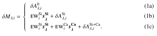 After finding
  and the
  by a least-squares minimization over all SNe from Eq. (1b), with an asymmetrical 2σ clipping, is kept constant and
  and the
  are then computed in the same manner. An example of the fit using ewSi for the B-band is given is Fig. 1 (solid line),
  being the correction applied to find the
  .
.
3.2. The empirical reddening law
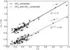 |
Fig. 2 Relation between δAU and δAV after ewSi correction (triangles up) and after ewSi and ewCa corrections (triangles down). The δAU are displayed with an added arbitrary constant. The ellipses represent the full measured covariance matrix between the two bands. They are enlarged by the additional subtraction error after ewCa correction. The result of the fits are also displayed. The |


Because we expect the relation between the δAλ to be linear for dust extinction, as shown in Fig. 2 for the U- and V-bands, we model the empirical reddening law as 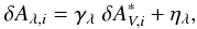 (2)where δAλ,i are the measured values, the slopes γλ ( =
  ) the reddening law coefficients,
  the fitted relative extinction for the SN i, and ηλ a free zero point. , γλ and ηλ are obtained by a χ2 fit using the full wavelength covariance matrix Ci of the δAλ,i measurements. However, the data are more dispersed than their measurement error (Fig. 2), and another source of dispersion must be introduced. We adopt an iterative approach by using the fit residuals,
 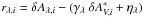 , to determine the covariance remaining after accounting for the measurement error covariance, Cλ1λ2,i. This empirical covariance matrix, D, is given by
 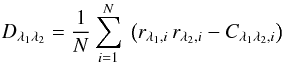 (3)where N is the number of SNe. In the next iteration, the total covariance matrix is given by Ci + D. We have checked that the converged matrix does not depend on initial conditions.
4. Results
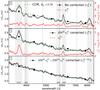 |
Fig. 3 Black: reddening law presented as |

4.1. EWSi and EWCa impacts on the derived extinction law
Results for the SED correction vector, sλ, and the reddening law, γλ, are presented in Fig. 3 for different assumptions about the number of intrinsic components. If SNe were perfect standard candles affected only by dust as assumed by Eq. (1a) and Fig. 3a, the empirical reddening law  would be a CCM-like law with an average RV for our galaxy sample. However, clearly exhibits small-scale SN-like features. These features correlate strongly with some of the features in the ewSi correction spectrum,
  , derived via Eq. (1b) and illustrated in red in Fig. 3a.
The reddening law obtained after ewSi correction (Fig. 3b) is closer to a CCM law, except in the Ca ii H&K and IR triplet, and the Si ii λ6355 region. This indicates the presence of a second source of intrinsic variability. We select ewCa to trace a second spectral correction vector,  (Eq. (1c)), since Ca is clearly a major contributor to the observed variability and ewCa and ewSi also happen to be uncorrelated (ρ = 0.06 ± 0.12). As shown in Fig. 3b, does a good job of reproducing the shape of the deviation of
  relative to the CCM law.
The mean reddening law,  , obtained after the additional correction by ewCa (Fig. 3c) is a much smoother curve with small residual features and agrees well with a CCM extinction law. Thus it appears that these two components can account for SN Ia spectral variations at optical wavelengths. Any intrinsic component that might remain would have to be largely uncorrelated with SN spectral features fixed in wavelength, as well as being coincidentally compatible with a CCM law.
4.2. RV determination
We apply the same treatment as above to our UBVRI-like synthetic photometric bands, and find agreement with the spectral analysis, as shown by the black points in the three panels in Fig. 3. After the ewSi correction (Eq. (1b), Fig. 3b), the U- and I-band values deviate significantly from a CCM law, which is recovered after the full ewSi and ewCa correction (Eq. (1c), Fig. 3c). The empirical fit presented in Sect. 3.2 can be forced to follow a CCM extinction law by substituting 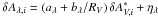 , where aλ and bλ are the wavelength-dependent parameters given in Cardelli et al. (1989) and O’Donnell (1994), and a single RV is fit over all bands. This fit applied to
  leads to an average RV = 2.78 ± 0.34 for the SN host galaxies in our sample. This value is compatible with the Milky Way average of RV = 3.1 The quoted uncertainty is statistical and derived with a jackknife procedure, removing one supernova at a time.
We tested the robustness of our RV determination in several ways. Since the sλ are measured in sequence, each one using the corrected magnitudes from the previous step, we swap the order in which the correction is applied, and find RV = 2.70. Using the whole sample to compute the sλ instead of applying a 2σ clipping cut leads to RV = 2.79, which shows the small influence of clipping at this stage. Host galaxy subtraction is performed using the full spatio-spectral information from the host obtained after the SN Ia has faded, and we do not see evidence for residual host galaxy features in our spectra. The measurement covariance matrix Ci depends on the assumed calibration accuracy: for the present result, this is estimated from repeated measurements of standard stars. Another estimate can be obtained from the residuals to a SALT2 light-curve fit. Using this in Ci values leads to RV = 2.76. The stability of the result with respect to our choice of bandpasses is checked by removing one band at a time, and we obtain a rms of ± 0.23 around the mean result. Finally, a Monte Carlo simulation was performed using the converged γλ,  , ηλ and dispersion matrix D as an input, and setting RV = 2.78. The δAλ,i are then randomly generated adding Gaussian noise with covariance Ci + D. Over 100 generations, the D matrix is recovered with a maximal bias of 5% on the diagonal elements and the mean fitted value is RV = 2.68 ± 0.03, indicating that, if anything, our method slightly underestimates RV.
5. Discussion
In this work, we selected ewSi as a first variable for correction because it provides a good proxy for x1, and it because is a model-independent variable. In our data-set the Pearson correlation coefficient of ewSi with x1 is − 0.83 ± 0.04 (Fig. 1), which confirms the result found in Arsenijevic et al. (2008). Computing the Hubble residuals in the B-band using (x1,c) or (ewSi,c) to standardize SNe both lead to a dispersion of residuals of 0.16 mag, also confirming this result. We find that ewSi is uncorrelated with c (ρ = −0.04 ± 0.12, Fig. 1), contrary to the recent claim by Nordin et al. (2010). Because ewSi and x1 are highly correlated, it is possible to redo the analysis with x1 in place of ewSi. The resulting SED correction vector  is similar to
  , and the conclusions identical, yielding RV = 2.69.
Computing the Hubble residuals with (ewSi,ewCa,c) to standardize supernovae leads to a dispersion of 0.15 mag, which is a small improvement. Indeed, we do observe a correlation of ewCa and c, with ρ = 0.34 ± 0.10. This correlation is even increased to ρ = 0.50 when c is computed with a U-band in addition to BVR in the light-curve fit. This shows that c contains an intrinsic component, and that the SALT2 analysis is already accounting for some of this Ca effect. This is illustrated in Fig. 3b: the SALT2 color model is derived taking into account a variability measured by one intrinsic parameter only, and thus can be compared to  . The observed U-band contribution in broad filters explains the UV rise in the empirical color models. The presence of a second intrinsic parameter induces an increased variability in the UV, as was already noticed by Ellis et al. (2008), but without a clear attribution to the Ca ii H&K line.
Much lower effective RV values have been found previously: RV = 1.1 in Tripp (1998), RV = 2.2 in Kessler et al. (2009); Guy et al. (2010) and RV ≈ 1 − 2 in Folatelli et al. (2010). These values were derived accounting only for one intrinsic parameter beyond color. If we derive an effective value after the sole ewSi correction to mimic these analyses, we obtain RV = 3.1, so the explanation for the difference has little to do with the number of intrinsic parameters entering the correction. This difference is explained by the assumption on the dispersion matrix. Indeed, if we instead use the one of Guy et al. (2010), corresponding to an rms between 0.09 and 0.11 mag on the diagonal, and all off-diagonal terms with an identical rms of 0.09 mag, we obtain RV = 1.86. This value is representative of previous analyses, but the matrix used is incompatible with our best-fit matrix. D has diagonal values of 0.07, 0.04, 0.05, 0.05 and 0.10 for UBVRI respectively, lower than the values quoted by Guy et al. (2010). However, while adjacent bands are correlated in our matrix, an anti-correlation growing to − 1 when the wavelength difference increases is observed for other bands, which implies a large color dispersion. As shown by Freedman et al. (2009) and Kessler et al. (2009), increasing the color dispersion leads to a higher RV value. This long-range anti-correlation implies that uncorrected variability in the SN spectra and/or the reddening law remains.
6. Conclusions
Equivalent widths are essentially independent of host reddening and provide a handle on the intrinsic properties of the SNe Ia.
In particular, ewSi measured at maximum light is confirmed to be as powerful as stretch. After correction for this intrinsic contribution to the magnitude, we derived a reddening law and proposed a natural method to assess the dispersion caused by additional fluctuations. We found that this empirical reddening law is affected by features linked to the SN physics, and showed that the Ca ii H&K line provides a second intrinsic variable that is uncorrelated with ewSi or x1. Correcting Hubble residuals with ewSi and ewCa leads to a reddening law consistent with a canonical CCM extinction law, while adding a dispersion in colors during the fit leads to a value of RV close to the Milky Way value of 3.1. Owing to the coupling of RV with the residual dispersion matrix, the derived value of RV may be affected as the remaining variability becomes better understood and corrected. Our plan to study the same SNe Ia over a range of phases should help address this issue. The evolution of SNe Ia will be one of the main limitations to their use in precision cosmology surveys at high redshift. Our findings show that the accurate measurements of the Ca ii H&K line provides an additional tool to improve the separation of dust and intrinsic variability. The presence of remaining scatter offers the possibility of improvements in the future.
Online material
Supernovae used in this work, including synthetic magnitudes after phase correction δMλ, SALT2 fit parameters x1 and c, equivalent widths ewSi and ewCa in Å and phases in days.
Acknowledgments
We are grateful to the technical and scientific staff of the University of Hawaii 2.2-m telescope, Palomar Observatories, and the High Performance Research and Education Network (HPWREN) for their assistance in obtaining these data. We also thank the people of Hawaii for access to Mauna Kea. This work was based in part on observations with UCO facilities (Keck and Lick 3 m) and NOAO facilities (Gemini-S (program GS-2008B-Q-26), SOAR, and CTIO 4 m). We thank UCO and NOAO for their generous allocations of telescope time. We thank Julien Guy for fruitful discussions on color law derivation as well as the anonymous referee and Alex Kim for constructive comments on the text. This work was supported in France by CNRS/IN2P3, CNRS/INSU, CNRS/PNC, and used the resources of the IN2P3 computer center. This work was supported by the DFG through TRR33 “The Dark Universe”, and by National Natural Science Foundation of China (grant 10903010). This work was also supported in part by the Director, Office of Science, Office of High Energy and Nuclear Physics and the Office of Advanced Scientific Computing Research, of the US Department of Energy (DOE) under Contract Nos. DE-FG02-92ER40704, DE-AC02-05CH11231, DE-FG02-06ER06-04, and DE-AC02-05CH11231; by a grant from the Gordon & Betty Moore Foundation; by National Science Foundation Grant Nos. AST-0407297 (QUEST), and 0087344 & 0426879 (HPWREN); by a Henri Chretien International Research Grant administrated by the American Astronomical Society; the France-Berkeley Fund; by an Explora Doc Grant by the Region Rhone Alpes; and the Aspen Center for Physics.
References
- Aldering, G., Adam, G., Antilogus, P., et al. 2002, SPIE Conf., 4836, 61 [Google Scholar]
- Arsenijevic, V., Fabbro, S., Mourão, A. M., et al. 2008, A&A, 492, 535 [NASA ADS] [CrossRef] [EDP Sciences] [Google Scholar]
- Bailey, S., Aldering, G., Antilogus, P., et al. 2009, A&A, 500, L17 [NASA ADS] [CrossRef] [EDP Sciences] [Google Scholar]
- Bronder, T. J., Hook, I. M., Astier, P., et al. 2008, A&A, 477, 717 [NASA ADS] [CrossRef] [EDP Sciences] [Google Scholar]
- Cardelli, J. A., Clayton, G. C., & Mathis, J. S. 1989, ApJ, 345, 245 [NASA ADS] [CrossRef] [Google Scholar]
- Cooke, J., Ellis, R. S., Sullivan, M., et al. 2011, ApJ, 727, L35 [NASA ADS] [CrossRef] [Google Scholar]
- Ellis, R. S., Sullivan, M., Nugent, P. E., et al. 2008, ApJ, 674, 51 [NASA ADS] [CrossRef] [Google Scholar]
- Folatelli, G., Phillips, M. M., Burns, C. R., et al. 2010, AJ, 139, 120 [NASA ADS] [CrossRef] [Google Scholar]
- Freedman, W. L., Burns, C. R., Phillips, M. M., et al. 2009, ApJ, 704, 1036 [NASA ADS] [CrossRef] [Google Scholar]
- Guy, J., Astier, P., Baumont, S., et al. 2007, A&A, 466, 11 [NASA ADS] [CrossRef] [EDP Sciences] [Google Scholar]
- Guy, J., Sullivan, M., Conley, A., et al. 2010, A&A, 523, A7 [NASA ADS] [CrossRef] [EDP Sciences] [Google Scholar]
- Hicken, M., Challis, P., Jha, S., et al. 2009, ApJ, 700, 331 [NASA ADS] [CrossRef] [Google Scholar]
- Jha, S., Riess, A. G., & Kirshner, R. P. 2007, ApJ, 659, 122 [NASA ADS] [CrossRef] [Google Scholar]
- Kessler, R., Becker, A. C., Cinabro, D., et al. 2009, ApJS, 185, 32 [NASA ADS] [CrossRef] [Google Scholar]
- Nordin, J., Ostman, L., Goobar, A., et al. 2010 [arXiv:1012.4430] [Google Scholar]
- O’Donnell, J. E. 1994, ApJ, 422, 158 [NASA ADS] [CrossRef] [Google Scholar]
- Phillips, M. M. 1993, ApJ, 413, L105 [NASA ADS] [CrossRef] [Google Scholar]
- Tripp, R. 1998, A&A, 331, 815 [NASA ADS] [Google Scholar]
- Walker, E. S., Hook, I. M., Sullivan, M., et al. 2011, MNRAS, 410, 1262 [NASA ADS] [CrossRef] [Google Scholar]
- Wang, X., Filippenko, A. V., Ganeshalingam, M., et al. 2009, ApJ, 699, L139 [NASA ADS] [CrossRef] [Google Scholar]
All Tables
Supernovae used in this work, including synthetic magnitudes after phase correction δMλ, SALT2 fit parameters x1 and c, equivalent widths ewSi and ewCa in Å and phases in days.
All Figures
|
Fig. 1 Correlations of ewSi, SALT2 x1 (top left) and c (top right) parameters and measured peak absolute magnitude up to a constant term, δMB (bottom). The open circles in the bottom panel are the data points excluded from the fit, which is displayed as a solid line. |
| In the text | |
|
Fig. 2 Relation between δAU and δAV after ewSi correction (triangles up) and after ewSi and ewCa corrections (triangles down). The δAU are displayed with an added arbitrary constant. The ellipses represent the full measured covariance matrix between the two bands. They are enlarged by the additional subtraction error after ewCa correction. The result of the fits are also displayed. The |
| In the text | |
|
Fig. 3 Black: reddening law presented as |
| In the text | |
Current usage metrics show cumulative count of Article Views (full-text article views including HTML views, PDF and ePub downloads, according to the available data) and Abstracts Views on Vision4Press platform.
Data correspond to usage on the plateform after 2015. The current usage metrics is available 48-96 hours after online publication and is updated daily on week days.
Initial download of the metrics may take a while.