© ESO, 2011

1. Introduction

Around solar minima the global distribution of the solar wind exhibits a simple bimodal structure: a band around the helioequator with an angular width ~50° of the slow wind (speed v ≲ 500 km   s^-1) is sandwiched between the high-latitude fast winds (v ≳ 650 km   s^-1) (e.g., Plate 1 in McComas et al. 2000). This picture was established indirectly by interplanetary scintillation (IPS) measurements in 1974 and 1985, corresponding to the minimum of solar cycles (SC) 20 and 21, respectively (Kojima & Kakinuma 1990). However, it became definitive only when Ulysses finished the first polar orbit, which encompasses the minimum of SC 22 (McComas et al. 2000). The bimodal picture continued for the SC 23 minimum as shown by Ulysses during its third polar orbit (McComas et al. 2008; Ebert et al. 2009).

What makes the fast solar wind fast and slow wind slow? In the context of the Ulysses measurements, what produces the pronounced latitudinal variation of v? Considering the well-established empirical relation between v and the coronal expansion rate f_c of flow tubes (Wang & Sheeley 1990), one may expect that the speed profile results from the differences in f_c of tubes reaching different latitudes in interplanetary space. Models that incorporate heating rates closely related to the magnetic field B indeed suggest that varying the spatial distribution of B, or equivalently that of the expansion rate, can result in considerable changes in wind parameters (for a summary of geometrical models, see Cranmer 2005; for more recent models adopting empirical heating terms, see Wang 2011). For instance, the most recent models based on the anisotropic turbulence, which self-consistently accommodate the heating from interactions of counter-propagating Alfvén waves, indicate that by varying the B profile alone, the modeled latitudinal dependence of wind speed at 1 AU can agree fairly well with the Ulysses measurements (Fig. 12 in Cranmer et al. 2007).

While the f_c − v relationship is strikingly robust, the significant spread in v in a given f_c interval means that v is a function of more than f_c, and the angular distance θ_b of the field line footpoint to its nearest coronal hole boundary was proved a good candidate for this additional factor (Arge et al. 2004). For a given f_c, the smaller θ_b, the lower is the speed. Because one naturally expects that the open field line becomes increasingly curved while its footpoint becomes closer to the coronal hole boundary, a natural alternative to θ_b would be the shape of field lines. Surprisingly, the possible effect of field line curvature has not been examined yet. Instead, the available turbulent-heating-based models tend to assume a radially directed flow tube, even though the non-radial tube expansion has been examined in considerable detail  (e.g., Chen & Hu 2002; Cranmer et al. 2007; Wang 2011).

The aim of this study is to examine how the field line shape affects the solar wind parameters in general, and whether it helps reproduce the Ulysses measurements in particular. It should be noted that while fully multi-dimensional models incorporating turbulent or empirical heating rates (e.g., Usmanov et al. 2000; Chen & Hu 2001; Li et al. 2004; Cohen et al. 2007; Lionello et al. 2009; Feng et al. 2010; van der Holst et al. 2010) certainly have taken account of both a non-radial expansion and the field line curvature, the two effects cannot be separated. Therefore we choose to solve the transport equations along field lines in a prescribed magnetic field configuration typical of the solar minimum corona, thereby allowing us to switch on and off the effect of the field line shape. The solar wind model we employ incorporates a physically motivated boundary condition, distinguishes between electrons and protons, adopts reasonably complete energy equations including radiative losses, electron heat conduction, and the solar wind heating from parallel propagating turbulent Alfvén waves.

The paper is organized as follows. In Sect. 2 we give a brief overview of the model and describe how it is implemented. The numerical solutions are then presented in Sect. 3. Finally, Sect. 4 summarizes the results, ending with some concluding remarks.

2. Model description and solution method

We consider a time-independent electron-proton solar wind flowing in the meridional plane and incorporating turbulent heating from Alfvén waves. Since the equations are quite well-known, we simply note that the mass or energy exchange between neighboring flow tubes is prohibited, permitting the decomposition of the vector equations (e.g., Eqs. (2) to (7) in Li et al. 2005, and references therein) into a force balance condition transverse to B and a set of conservation equations along it. For mathematical details, please see the appendix of Li & Li (2006). Here we replace the former with a prescribed magnetic field, and treat only the conservation equations in detail. The Alfvén waves are assumed to propagate along B and to be dissipated at the Kolmogorov rate Q_wav = ρδv³/L_c, where ρ = nm_p is the mass density with n and m_p being the number density and proton mass, respectively. Moreover, δv is the rms value of the wave velocity fluctuations, and L_c the correlation length. By standard treatment, the wave heating Q_wav goes entirely to protons, and L_c = L_c0(B₀/B)^1/2, where the subscript 0 denotes values at the field line footpoint at the Sun. This form of dissipation and its variants, first proposed by Hollweg (1986), have been a common practice in solar wind modeling ever since (see e.g., the review by Hollweg & Isenberg 2002).

The conservation equations along an arbitrary magnetic line of force read $\begin{array}{ccc}& & \frac{{\mathrm{(}\mathit{nv}{\mathit{A}}^{\mathrm{)}}}^{\mathrm{\prime }}}{\mathit{A}}\mathrm{=}\mathrm{0}\mathit{,}\\ & & \mathit{v}{\mathit{v}}^{\mathrm{\prime }}\mathrm{+}\frac{{\mathit{p}}_{\mathrm{p}}^{\mathrm{\prime }}}{\mathit{\rho }}\mathrm{+}\frac{{\mathit{p}}_{\mathrm{e}}^{\mathrm{\prime }}}{\mathit{\rho }}\mathrm{-}{\left(\frac{\mathit{G}{\mathit{M}}_{\mathrm{\odot }}}{\mathit{r}}\right)}^{\mathrm{\prime }}\mathrm{=}\frac{\mathit{F}}{\mathit{\rho }}\mathit{,}\\ & & {\mathit{T}}_{\mathrm{s}}^{\mathrm{\prime }}\mathrm{+}\mathrm{(}\mathit{\gamma }\mathrm{-}\mathrm{1}\mathrm{)}{\mathit{T}}_{\mathrm{s}}\mathrm{\left[}\ln \mathrm{\right(}\mathit{vA}\mathrm{)}{\mathrm{]}}^{\mathrm{\prime }}\mathrm{=}\frac{\mathit{\gamma }\mathrm{-}\mathrm{1}}{\mathit{n}{\mathit{k}}_{\mathrm{B}}\mathit{v}}[\frac{\mathit{\delta }{\mathit{E}}_{\mathrm{s}}}{\mathit{\delta t}}\mathrm{+}{\mathit{Q}}_{\mathrm{s}}\mathrm{-}\mathit{L}\mathrm{-}\frac{{\left({\mathit{q}}_{\mathrm{s}}\mathit{A}\right)}^{\mathrm{\prime }}}{\mathit{A}}]\mathit{,}\\ & & \frac{{\mathrm{(}{\mathit{F}}_{\mathrm{w}}{\mathit{A}}^{\mathrm{)}}}^{\mathrm{\prime }}}{\mathit{A}}\mathrm{+}\mathit{vF}\mathrm{=}\mathrm{-}{\mathit{Q}}_{\mathrm{wav}}\mathit{,}\end{array}$\arraycolsep1.75ptwhere v is the wind speed, A ∝ 1/B is the cross-sectional area of the flux tube, and the prime ′ denotes the derivative with respect to the arc length l, measured from the footpoint of the field line. The species pressures p_s (s = e,p) are related to species temperatures T_s via p_s = nk_BT_s in which k_B is the Boltzmann constant. The gravitational constant is denoted by G, and M_⊙ is the mass of the Sun. Note that the gravitational acceleration is put in the form of a directional derivative. In addition, the force density acting on the fluid is caused by Alfvén waves, $\mathit{F}\mathrm{=}\mathrm{-}{\mathit{p}}_{\mathrm{w}}^{\mathrm{\prime }}$ where p_w = ρδv²/2 is the wave pressure. The adiabatic index γ = 5/3, and δE_s/δt represents the energy exchange rates of species s due to Coulomb collisions with the other species. To evaluate them, we take the Coulomb logarithm to be 23. For simplicity, the proton heat flux is neglected (q_p = 0), whereas the electron one is taken to be the Spitzer law ${\mathit{q}}_{\mathrm{e}}\mathrm{=}\mathrm{-}\mathit{\kappa }{\mathit{T}}_{\mathrm{e}}^{\mathrm{5}\mathit{/}\mathrm{2}}{\mathit{T}}_{\mathrm{e}}^{\mathrm{\prime }}$ where κ = 7.8 × 10^-7 erg K^−7/2 cm^-1 s^-1. Moreover, the heating rates applied to species s is denoted by Q_s. For the protons, one has Q_p = Q_wav. On the other hand, optically thin radiative losses are accounted for by the term L, which is included in the electron version of Eq. (3) and is described by the parametrization scheme of Rosner et al. (1978). Some electron heating is also included, expressed by where is the magnitude and l_d the scale length of this heating. For simplicity, here we assume that this electron heating is associated with no momentum deposition. Equation (4) describes the wave evolution, in which F_w = p_w⁽3v + 2v_A⁾ is the wave energy flux density with ${\mathit{v}}_{\mathrm{A}}\mathrm{=}\mathit{B}\mathit{/}\sqrt{\mathrm{4}\mathit{\pi \rho }}$ the Alfvén speed.

Given the governing equations, one may say a few words on the effect of the magnetic field line shape before actually solving them. Consider the case, referred to as Case S, where we put dl = dr in ′ (note that ′ is also involved in q_e) and l = r − R_⊙ in Q_e. Here r is the heliocentric distance and R_⊙ the solar radius. As such, Case S differs from the original case, called Case C, only in that the field lines are straight in the former, but allowed to be curved in the latter. It then follows that if the wind energetics is not self-consistently considered, say, if one prescribes an r-distribution of the temperatures T_e and T_p, then Eqs. (1) and (2) indicate that no matter how curved the field line may be, the same r-profiles for n and v result. This applies even if the waves are considered as long as the wave dissipation is neglected. To understand this, one may readily derive from Eq. (4) a conservation law which reads (e.g. Hu et al. 1997) $\begin{array}{ccc}\frac{{\mathrm{(}\mathit{\omega S}{\mathit{A}}^{\mathrm{)}}}^{\mathrm{\prime }}}{\mathit{A}}\mathrm{=}\mathrm{-}\mathrm{(}\mathrm{1}\mathrm{+}{\mathit{M}}_{\mathrm{A}}\mathrm{)}{\mathit{Q}}_{\mathrm{wav}}\mathit{,}& & \end{array}$(5)where ωS = 2p_wv_A(1 + M_A) is the wave action flux density, and M_A = v/v_A is the Alfvénic Mach number. If Q_wav = 0, one finds that ωSA is a constant, enabling the wave pressure p_w to be expressed as a functional of flow parameters as well as B. As such multiplying Eqs. (1) and (2) by a factor dl/dr does not invalidate the equal signs. This means that any two field lines that have identical radial distributions of B,T_e and T_p will yield identical radial distributions of n,v and p_w, provided that the base values for n and δv are the same for the two lines. However, if the energy equation is explicitly considered, as we will do, and the adopted heating rates play a role in determining the solar wind mass flux, then the field line shape will likely play a role (see also the discussion section).

For the meridional magnetic field, we adopt the Banaszkiewicz et al. (1998) model for which we use the reference values [Q,K,a₁] = [1.5,1,1.538]. This set of parameters is supported by images obtained with the instruments on board the SOlar and Heliospheric Observatory (SOHO) spacecraft at solar minimum (see e.g., Fig. 1 in Forsyth & Marsch 1999), and has found extensive applications in solar wind models (e.g., Hackenberg et al. 2000; Cranmer et al. 2007; Li & Li 2008). Another parameter M, which controls the magnetic field strength, is chosen such that B at the Earth orbit is 3.5γ, consistent with Ulysses measurements (Smith & Balogh 1995; also Smith 2011).

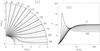Fig. 1 Adopted meridional magnetic field configuration in the corona. a) A quadrant is shown where the magnetic axis points upward, and the thick contours delineate the lines of force for which the expansion factors f = (A/A0)(R⊙/r)2 are plotted in b) as a function of heliocentric distance r. The field lines are labeled with the colatitude at which they intersect the Earth orbit (1 AU). Here A denotes the cross-sectional area of the flow tube, the subscript 0 represents values at the inner boundary R⊙.

The meridional magnetic field configuration is depicted in Fig. 1a, where the thick contours indicate the lines of force along which we compute the expansion factor f = (A/A₀)(R_⊙/r)², given in Fig. 1b. The field lines are labeled with the colatitude at which the lines are located at 1 AU. From Fig. 1a one can see that the open field lines occupy only a minor fraction of the solar surface, with colatitudes θ ≤ 30° to be specific. If one identifies this area as the coronal hole (CH) (see e.g., Wang 2011), one can indeed see that when their footpoints approach the CH boundary, the open field lines become progressively more curved. Furthermore, Fig. 1b shows that while in the inner corona, say at r = 1.7 R_⊙, the expansion factor f increases when the field lines become closer to the CH edge, the opposite is true at large distances, say r ≳ 20 R_⊙. As was first pointed out by Wang & Sheeley (1990), this tendency is due to the inclusion of the current sheet component in the magnetic field, and the low densities in the fast wind in interplanetary space were attributed to that flow tubes originating near the CH center experienced the most significant net expansion.

Given a B profile along a field line, the governing equations are put in a time-dependent form, discretized onto a non-uniformly spaced grid, and then advanced in time from an arbitrary initial state by a fully implicit scheme (Hu et al. 1997) until a steady state is reached, which is then taken as our solution. For the solutions found, the mass, momentum, and energy are found to be conserved to better than 1%. At the top boundary (1 AU), all flow parameters are linearly extrapolated for simplicity. At the base (1 R_⊙) the flow speed v is determined by mass conservation, whereas the species temperatures are fixed at T_e0 = T_p0 = T₀ = 5 × 10⁵ K, corresponding to mid-transition region. Because the processes taking place below this level should influence the mass supply to the solar wind (e.g., Hansteen & Leer 1995; Lie-Svendsen et al. 2002), they should be taken into account and can be well represented by the radiation equilibrium boundary (REB) condition (Withbroe 1988; Lionello et al. 2001). The REB condition translates into n₀ = 4.8 × 10³q_e0 in cgs units for our chosen T₀. As such, the base density n₀ is not fixed but allowed to adjust to the downward heat flux, which in turn depends on how the fluid is heated close to the base. Without the basal electron heating, the T_e gradient and hence the electron heat flux density q_e0 at the base are too low, leading to n₀T₀ ≪ 1.6    ×    10¹⁴ cm^-3 K, the value inferred from measurements with the Solar Ultraviolet Measurements of Emitted Radiation (SUMER) on SOHO for coronal holes (Warren & Hassler 1999). The values adopted for Q_e are  erg cm^-3 s^-1, and l_d = 0.06 R_⊙. With such a short scale length, Q_e rapidly gives way to the more gradual proton heating Q_wav, for which we use a base wave amplitude δv₀ = 27 km   s^-1 and a base value for the correlation length L_c0 of 1.5 × 10⁴ km. (Note that even though this L_c0 translates into approximately 0.02 R_⊙, it does not mean that the wave dissipation is extremely concentrated at the base. A length scale comparable to l_d involved in Q_e can be given by $\mathrm{|}{\mathit{Q}}_{\mathrm{wav}}\mathit{/}{\mathit{Q}}_{\mathrm{wav}}^{\mathrm{\prime }}\mathrm{|}$, for which one finds a value ranging from 0.086 R_⊙ at the base to 0.59 R_⊙ at 2 R_⊙ for the solution labeled case C in Fig. 2.)

3. Numerical results

To examine the extent to which the wind parameters are affected by the field line shape, we will compare solutions that incorporate the curvature effect (Case C) and those that neglect it (Case S).

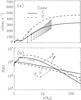Fig. 2 Alfvén wave-turbulence-based solar wind models incorporating effects of field line shape. Radial profiles are shown for a) the solar wind speed v, and b) the electron and proton temperatures Te and Tp. The curved (straight) case in which the field line shape is considered (neglected) is given by the solid (dashed) lines. In a), the asterisks indicate the sonic point where v equals the effective sonic speed cS defined by Eq. (6), while the vertical bars represent wind speeds measured by tracking small density inhomogeneities (blobs) in SOHO/LASCO images as given by Wang et al. (2000). The triangles in b) give the hydrogen kinetic temperatures derived from H I Lyα measurements with SOHO/UVCS for a typical solar minimum streamer (Strachan et al. 2002).

Figure 2 presents the radial profiles of (a) the wind speed v and (b) the electron and proton temperatures T_e and T_p for the solutions computed along the tube labeled 88 in Fig. 1a. For this field line the effect of the field line curvature is almost maximal. The solid and dashed curves correspond to Cases C and S, respectively. The asterisks in Fig. 2a refer to the sonic point where v equals the effective sound speed c_S given by (e.g., Eq. (36) in Hackenberg et al. 2000) $\begin{array}{ccc}{\mathit{c}}_{\mathrm{S}}^{\mathrm{2}}\mathrm{=}\frac{{\mathit{k}}_{\mathrm{B}}}{{\mathit{m}}_{\mathrm{p}}}\mathrm{(}{\mathit{T}}_{\mathrm{e}}\mathrm{+}{\mathit{T}}_{\mathrm{p}}\mathrm{)}\mathrm{+}\frac{{\mathit{p}}_{\mathrm{w}}}{\mathit{\rho }}\frac{\mathrm{1}\mathrm{+}\mathrm{3}{\mathit{M}}_{\mathrm{A}}}{\mathrm{2}\mathrm{(}\mathrm{1}\mathrm{+}{\mathit{M}}_{\mathrm{A}}\mathrm{)}}\mathrm{·}& & \end{array}$(6)Moreover, in Fig. 2a the vertical bars give the range of wind speeds derived by tracking a collection of small inhomogeneities (the blobs) in images obtained with the Large Angle Spectrometric COronagraph (LASCO) on board SOHO (Wang et al. 2000). The triangles in Fig. 2b represent the hydrogen kinetic temperatures derived from the H I Lyα profiles measured with the UltraViolet Coronagraph Spectrometer (UVCS) on SOHO for a typical solar minimum streamer (Strachan et al. 2002).

The solution for Case C (solid curves) agrees well with available measurements. For instance, the model yields the following parameters at 1 AU: v_E = 333 km   s^-1, (nv)_E = 3.65 × 10⁸ cm²   s^-1, T_e = 1.4 × 10⁵ K and T_p = 2.7 × 10⁴ K, all of which match the in-situ measurements by both Helios (Schwenn 1990) and Ulysses (McComas et al. 2000, 2008; Ebert et al. 2009) of the low latitude slow winds. Here the subscript E denotes the Earth orbit. Figure 2a indicates that the wind speed starts with 6.4 km   s^-1 at the base, which is in line with the Doppler speed measured with Ne VIII (e.g., Xia et al. 2003), whose formation temperature is close to our base temperature. The speed profile is not monotonic but possesses a local minimum at 1.63 R_⊙ where v = 25.1 km   s^-1. The sonic point, denoted by r_C, is located at 4.15 R_⊙. Between 3 and 20 R_⊙ the computed speeds are in line with the blob measurements. Moreover, for r ≲ 3 R_⊙ the modeled v is no higher than 98.8 km   s^-1, which would be below the sensitivity of the Doppler dimming of H I Lyα (Kohl et al. 2006), and in this sense is compatible with the fact that there is not much empirical knowledge about the proton speed in the inner portion of the slow wind. Moving to Fig. 2b one may see that because of the applied electron heating both T_e and T_p increase near the base. At 1.19 R_⊙ the electron temperature T_e attains its maximum of 9.8 × 10⁵ K. Below this height, T_e and T_p stay close to each other owing to Coulomb coupling. However, while T_e decreases monotonically with distance above this height, T_p further increases to 2.14 × 10⁶ K at 1.6 R_⊙ beyond which T_p declines with a slope steeper than T_e and is overtaken by T_e at 30.1 R_⊙. In the range from 1.75 to 5.11 R_⊙ the modeled proton temperature reproduces the H I measurements fairly satisfactorily, which indicates that the heating mechanism we employ performs well in heating the inner solar wind.

Compared with Case C, at 1 AU Case S yields a significantly higher proton speed and a substantially lower proton flux density. The parameters at 1 AU now read v_E = 461 km   s^-1, (nv)_E = 3.14 × 10⁸ cm²   s^-1, T_e = 7.5 × 10⁴ K, and T_p = 4.65 × 10⁴ K. In addition, Case S yields a sonic point at r_C = 3.24 R_⊙, closer to the Sun than in Case C. The differences between the temperatures in the two cases can be readily understood by examining Eq. (3). A higher speed in Case S leads to a more prominent adiabatic cooling (the second term on the left-hand side), which accounts for a steeper, negative T_e gradient and hence a lower asymptotic T_e; on the other hand, while the same also happens to protons, the reduced proton flux results in a higher Q_wav/(nv), which leads to a steeper, positive T_p gradient and eventually a higher asymptotic T_p. However, the question remains as to how neglecting the curvature of the field line leads to the changes in the proton speed and flux? This is understandable if one follows the comprehensive discussion by Leer & Holzer (1980): the more energy is deposited in the subsonic region of the flow, the higher the proton flux; and the larger the energy deposition per particle, the higher the terminal speed. Let us first examine the subsonic physics, from R_⊙ to the sonic point r_C. The contribution from the electron heating, measured as an energy flux density scaled to 1 AU ${{}^{\mathrm{\int }}\mathit{R}_{\mathrm{\odot }}}_{{\mathit{r}}_{\mathrm{C}}}^{}{\mathit{Q}}_{\mathrm{e}}\mathrm{(}\mathit{A}\mathit{/}{\mathit{A}}_{\mathrm{E}}\mathrm{)}\mathrm{d}\mathit{l}$, increases only slightly from 0.3 in Case C to 0.337 in Case S (here and hereafter the energy flux densities are in  erg   cm^-2   s^-1). However, the effect of energy addition to protons, which eventually derives from Alfvén waves since ${{}^{\mathrm{\int }}\mathit{R}_{\mathrm{\odot }}}_{{\mathit{r}}_{\mathrm{C}}}^{}\mathrm{(}{\mathit{Q}}_{\mathrm{p}}\mathrm{+}\mathit{vF}\mathrm{)}\mathrm{(}\mathit{A}\mathit{/}{\mathit{A}}_{\mathrm{E}}\mathrm{)}\mathrm{d}\mathit{l}\mathrm{=}{\mathit{F}}_{\mathrm{w}}\mathit{A}\mathit{/}{\mathit{A}}_{\mathrm{E}}{\mathrm{|}}_{{\mathit{R}}_{\mathrm{\odot }}}^{{\mathit{r}}_{\mathrm{C}}}$, reduces more significantly from 1.089 in Case C to 0.931 in Case S. And this reduction is a direct consequence of the field line shape. To see this, we note that the wave action Eq. (5) is a proper starting point, because its right-hand side (RHS) evaluates the consequence of the “genuine” dissipation while its LHS involves the wave ponderomotive force, which also contributes to the wave energy loss. Without dissipation, we saw that the field line shape is unable to make the radial distributions different in Case C from those in Case S, even when the ponderomotive force is allowed for. Expressing Eq. (5) in the integral form yields $\begin{array}{ccc}\left(\mathit{\omega S}\frac{\mathit{A}}{{\mathit{A}}_{\mathrm{E}}}\right)|\begin{array}{}{\mathit{r}}_{\mathrm{C}}\\ {\mathit{R}}_{\mathrm{\odot }}\end{array}\mathrm{=}\mathrm{-}{\mathrm{\int }}_{{\mathit{R}}_{\mathrm{\odot }}}^{{\mathit{r}}_{\mathrm{C}}}\mathrm{(}\mathrm{1}\mathrm{+}{\mathit{M}}_{\mathrm{A}}\mathrm{)}\frac{\mathit{A}}{{\mathit{A}}_{\mathrm{E}}}{\mathit{Q}}_{\mathrm{wav}}\mathrm{d}\mathit{l}\mathit{.}& & \end{array}$(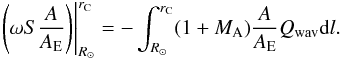7)Now that in general dl/dr > 1, which is particularly true in the inner flow where M_A ≪ 1, the RHS of Eq. (7) means that Q_wav of similar amount effectively contributes more to the wave energy reduction in the curved than in the straight case. Now let us discuss the asymptotic speeds. The net energy added to the solar wind, i.e., the electron heating plus wave dissipation plus enthalpy flux subtracted by radiative losses and the net electron heat flux flowing out of the computational domain, yields an energy flux scaled to 1 AU of 1.495 (1.553) in Case C (S). Divided by the proton flux density, this gives 0.41 (0.495) × 10^-8 erg per particle in Case C (S), which explains the higher terminal speed in Case S.

Now we return to the question what geometrical factor(s) besides the tube expansion may also affect the solar wind speed v. The comparison between the straight and curved cases shows that the field line shape could be one. In this regard, the physical basis for the empirical relation found by Arge et al. (2004) may be simply that θ_b, which measures how far the open field line footpoint is away from the coronal hole boundary, also characterizes the field line shape.

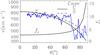Fig. 3 Distribution with colatitude θ of the computed solar wind speed v at 1 AU and the coronal expansion factor fc of the flow tube intersecting the Earth orbit at θ. The model result incorporating (neglecting) the field line shape, called Case C (S), is given by the solid (dashed) line. They are obtained by varying the flow tube alone but keeping all other parameters unchanged. Cases C and S both take the radial variation of the magnetic field strength into account, and differ from each other only in that Case C considers the field line shape whereas Case S neglects it. The blue continuous curve gives the daily averaged speed measurements by Ulysses during the first half of its latitude scan from Sep. 12, 1994 to Mar. 4, 1995. As for fc, it is taken to have the value of f at a heliocentric distance of 1.7 R⊙.

What role does the shape of field lines play in shaping the latitudinal profile of the solar wind speed at 1 AU? This is examined in Fig. 3, which compares the speed profile in Case C (the solid curve) and in Case S (the dashed curve). The model results are obtained by varying only the flow tube along which the governing equations are solved, but keeping everything else untouched. In addition to the speed v at 1 AU, Fig. 3 also displays as a function of colatitude θ the coronal expansion factor f_c of the flow tube that reaches 1 AU at θ. Here f_c is defined as (A/A₀)(R_⊙/r_cor)², where r_cor is taken to be 1.7 R_⊙ (see Fig. 1b). For comparison, the solid curve in blue gives the daily averages of the Ulysses measurements of the wind speed during the first half of the fast latitude scan from Sep. 12, 1994 to Mar. 4, 1995. From Fig. 3 one can see that while the speed v in both models is inversely correlated with f_c, the results in Case C provide a stronger latitudinal variation. Indeed, the reduction in the wind speed caused by the field line shape is larger than 10% throughout the latitudinal range θ ≳ 70°, with the largest relative difference being 27.8%, which occurs close to the equator. Furthermore, without more tweaking of the heating parameters, such as varying the base values of the wave amplitude δv₀ and the correlation length L_c0 from tube to tube as was done by e.g., Li et al. (2004), the modeled latitudinal dependence for θ ≲ 70° is too strong to reproduce the measured profile for the fast wind. Despite this, the low-latitude portion of Fig. 3 indicates that in addition to a more pronounced coronal expansion rate, the field line curvature is also an important factor that makes the slow wind there slow.

4. Summary and concluding remarks

Both remote-sensing measurements using the interplanetary scintillation (IPS) technique and in-situ measurements by the Ulysses spacecraft show a latitudinal gradient in the wind properties, the speed in particular, at solar minimum conditions (Kojima & Kakinuma 1990; McComas et al. 2000, 2008). What makes the fast wind fast and the slow wind slow still seems elusive. While there exists a robust empirical correlation between the coronal expansion rate f_c of the flow tubes and the speeds v measured in situ (Wang & Sheeley 1990), a more detailed data analysis suggests that v depends on more than just f_c (Arge et al. 2004). We examined whether the non-radial shape of field lines, which naturally accompanies any non-radial expansion, could be an additional geometrical factor. To this end, we solved the transport equations for an electron-proton solar wind, which incorporate the heating from turbulent Alfvén waves dissipated at the Kolmogorov rate, along curved field lines given by the Banaszkiewicz et al. (1998) model, which is representative of a solar minimum corona. The shape of field lines was found to substantially influence the solar wind parameters, reducing the terminal speed by as much as ~130 km   s^-1  or up to 28%, compared to the straight case where field line curvature is neglected. And this effect was interpreted in the general framework of energy addition in the solar wind by Leer & Holzer (1980): compared with the straight case, even though the wave dissipation rates may be similar, the field line curvature enhances the effective wave energy deposition in the subsonic region of the flow, which results in a higher proton flux and a lower terminal proton speed. Our results suggest that the experimental finding by Arge et al. (2004) may be interpreted in view of the fact that flow tubes with identical coronal expansion rates may differ substantially in their curvature. On the other hand, even though the field line curvature is unlikely to affect the polar fast solar wind at solar minima, it does considerably help the wind at low latitudes become slow, which in turn helps to better reproduce the Ulysses measurements.

Could this effect have to do with the particular boundary conditions or the energy deposition mechanism employed here? This proves very unlikely. We tested cases where the inner boundary is placed at the lower transition region where T = 10⁵ K, or the “coronal base” where T = 10⁶ K. Adjusting the heating parameters in a way that realistic values can be obtained for the proton flux and asymptotic speed, and comparing solutions with field line curvature switched on and off, the conclusion is the same. On the other hand, using a different heating function where Q_p is given by the dissipation of some unspecified mechanical energy flux at a constant scale length, the conclusion is the same. Moreover, this effect is not related to the heat conduction, even though the effective electron heat conductivity is reduced by a factor dr/dl in the curved case. Indeed, turning off the electron heat flux, in which case we have to fix the base density though, we reach the same conclusion. All of these additional computations corroborate our interpretation that the changes brought forth by the field line shape are simply related to the differential arc-length dl involved in Eq. (7), whereby the more curved the field lines are in the subsonic region, the greater is the wave energy reduction there, hence the higher the proton flux, and with the total input energy flux barely changing, the lower the terminal proton speed. The effect of the field line shape therefore should happen in quite general situations where the wave dissipation rate Q_wav is not directly proportional to the spatial derivative of background parameters and the energy deposition in the subsonic region plays a significant role in determining the solar wind flux. From this perspective one may expect that the effect of field line curvature is not restricted to flow tubes rooted at any particular latitude on the Sun. Instead, it should play a role for any flow tube that is curved. Moreover, this effect should also exhibit some influence on the flow if one employs the anisotropic turbulence treatment of the Alfvén waves to incorporate the finite-wavelength non-WKB effects, as is actively pursued at present (Cranmer et al. 2007; Verdini et al. 2010). Compared with a radial one, a curved line of force is likely to enhance the non-WKB effect (i.e., reflection) in the near-Sun region (Fig. 16 in Heinemann & Olbert 1980). However, to predict what happens next is not as straightforward as what was done here. Let us neglect the wave dissipation for the moment, i.e., the waves interact with the flow only via their ponderomotive force. The enhanced reflection then tends to lead to a reduction of this force, and hence to a reduced mass flux as well as a lower terminal speed. Unlike the dissipationless case discussed in Sect. 2, this tendency exists both when the wind temperatures are prescribed (Fig. 10 in MacGregor & Charbonneau 1994) and when the wind energetics is self-consistently treated (Fig. 4 in Li & Li 2008). The case with turbulent dissipation is considerably more complicated. The enhancement of wave reflection in the subsonic flow means an enhancement of the ingoing component of the waves. With the turbulent dissipation trying to diminish both outgoing and reflected components to similar extents, a substantial fraction of the reflected component may end up in the supersonic portion of the flow, and its consequent dissipation may lead to a higher terminal speed with the mass flux barely altered. However, this is not the whole story because the ponderomotive force is altered in a similar fashion to the dissipationless case. As such, the net outcome has to be told by a detailed numerical study, which is beyond the scope of this paper. Nonetheless, it seems fair to say that if one tries to reproduce the Ulysses measurements, especially those of the slow solar wind at low latitudes, the field line shape has to be accounted for.

That said, let us say a few words on the situations where the curvature effects are unlikely to be important. This may happen, for instance, 1) in the spectral erosion scenario where the solar wind is heated by high-frequency Alfvén waves (with frequencies up to 10 kHz) that are directly launched by chromospheric magnetic reconnections, since now the dissipation rate is proportional to the directional derivative of the proton gyro-frequency and therefore the background magnetic field strength (Marsch & Tu 1997; Hackenberg et al. 2000); 2) in the scenario for the solar wind generation where both the energy F_w0 and mass injection F_m0 rates are fixed (e.g., Fisk 2003; Tu et al. 2005). To illustrate this, consider the scenario by Fisk (2003) where the energy and mass injection occurs at some level where the temperature is on the order of 1 MK, which means, roughly speaking, the contributions like enthalpy, heat flux and radiative losses may be neglected when considering the overall energy balance between the injection point and 1 AU. Evidently the

mass flux density at 1 AU is simply F_m0A₀/A_E, and from energy conservation it follows that the terminal proton speed is approximately $\sqrt{\mathrm{2}{\mathit{F}}_{\mathrm{w}\mathrm{0}}\mathit{/}{\mathit{F}}_{\mathrm{m}\mathrm{0}}\mathrm{-}\mathit{G}{\mathit{M}}_{\mathrm{\odot }}\mathit{/}{\mathit{R}}_{\mathrm{\odot }}}$. As such, the terminal mass flux density is determined by the net expansion of the flow tube from its footpoint to 1 AU, but the speed is related to neither the tube expansion nor the field line shape.

Acknowledgments

We thank the referee (Dr. Andrea Verdini) for his comments, which helped us clarify the possible effects of the magnetic field line shape on a turbulence-heated solar wind where the non-WKB effects are considered. The Ulysses data are obtained from the CDAWeb database. The SWOOPS team (PI: D. J. McComas) is gratefully acknowledged. This research is supported by the grant NNSFC 40904047, and also by the Specialized Research Fund for State Key Laboratories. Y.C. is supported by grants NNSFC 40825014 and 40890162, and LDX by NNSFC 40974105.

References

All Figures

Fig. 1 Adopted meridional magnetic field configuration in the corona. a) A quadrant is shown where the magnetic axis points upward, and the thick contours delineate the lines of force for which the expansion factors f = (A/A0)(R⊙/r)2 are plotted in b) as a function of heliocentric distance r. The field lines are labeled with the colatitude at which they intersect the Earth orbit (1 AU). Here A denotes the cross-sectional area of the flow tube, the subscript 0 represents values at the inner boundary R⊙.

In the text

Fig. 2 Alfvén wave-turbulence-based solar wind models incorporating effects of field line shape. Radial profiles are shown for a) the solar wind speed v, and b) the electron and proton temperatures Te and Tp. The curved (straight) case in which the field line shape is considered (neglected) is given by the solid (dashed) lines. In a), the asterisks indicate the sonic point where v equals the effective sonic speed cS defined by Eq. (6), while the vertical bars represent wind speeds measured by tracking small density inhomogeneities (blobs) in SOHO/LASCO images as given by Wang et al. (2000). The triangles in b) give the hydrogen kinetic temperatures derived from H I Lyα measurements with SOHO/UVCS for a typical solar minimum streamer (Strachan et al. 2002).

In the text

Fig. 3 Distribution with colatitude θ of the computed solar wind speed v at 1 AU and the coronal expansion factor fc of the flow tube intersecting the Earth orbit at θ. The model result incorporating (neglecting) the field line shape, called Case C (S), is given by the solid (dashed) line. They are obtained by varying the flow tube alone but keeping all other parameters unchanged. Cases C and S both take the radial variation of the magnetic field strength into account, and differ from each other only in that Case C considers the field line shape whereas Case S neglects it. The blue continuous curve gives the daily averaged speed measurements by Ulysses during the first half of its latitude scan from Sep. 12, 1994 to Mar. 4, 1995. As for fc, it is taken to have the value of f at a heliocentric distance of 1.7 R⊙.

In the text

References

- Arge, C. N., Luhmann, J. G., Odstrcil, D., Schrijver, C. J., & Li, Y. 2004, J. Atm. Solar-Terrestrial Phys., 66, 1295 [Google Scholar]
- Banaszkiewicz, M., Axford, W. I., & McKenzie, J. F. 1998, A&A, 337, 940 [NASA ADS] [Google Scholar]
- Chen, Y., & Hu, Y. Q. 2001, Sol. Phys., 199, 371 [NASA ADS] [CrossRef] [Google Scholar]
- Chen, Y., & Hu, Y. Q. 2002, Ap&SS, 282, 447 [NASA ADS] [CrossRef] [Google Scholar]
- Cohen, O., Sokolov, I. V., Roussev, I. I., et al. 2007, ApJ, 654, L163 [NASA ADS] [CrossRef] [Google Scholar]
- Cranmer, S. R. 2005, Solar Wind 11/SOHO 16, Connecting Sun and Heliosphere, 592, 159 [NASA ADS] [Google Scholar]
- Cranmer, S. R., van Ballegooijen, A. A., & Edgar, R. J. 2007, ApJS, 171, 520 [Google Scholar]
- Ebert, R. W., McComas, D. J., Elliott, H. A., Forsyth, R. J., & Gosling, J. T. 2009, J. Geophys. Res., 114(A01), 109 [Google Scholar]
- Feng, X., Yang, L., Xiang, C., et al. 2010, ApJ, 723, 300 [Google Scholar]
- Fisk, L. A. 2003, J. Geophys. Res., 108, 1157 [Google Scholar]
- Forsyth, R. J., & Marsch, E. 1999, Space Sci. Rev., 89, 7 [NASA ADS] [CrossRef] [Google Scholar]
- Hackenberg, P., Marsch, E., & Mann, G. 2000, A&A, 360, 1139 [NASA ADS] [Google Scholar]
- Hansteen, V. H., & Leer, E. 1995, J. Geophys. Res., 100, 21577 [NASA ADS] [CrossRef] [Google Scholar]
- Heinemann, M., & Olbert, S. 1980, J. Geophys. Res., 85, 1311 [NASA ADS] [CrossRef] [Google Scholar]
- Hollweg, J. V. 1986, J. Geophys. Res., 91, 4111 [Google Scholar]
- Hollweg, J. V., & Isenberg, P. A. 2002, J. Geophys. Res., 107, 1147 [CrossRef] [Google Scholar]
- Hu, Y. Q., Esser, R., & Habbal, S. R. 1997, J. Geophys. Res., 102, 14661 [NASA ADS] [CrossRef] [Google Scholar]
- Kohl, J. L., Noci, G., Cranmer, S. R., & Raymond, J. C. 2006, A&ARv, 13, 31 [NASA ADS] [CrossRef] [Google Scholar]
- Kojima, M., & Kakinuma, T. 1990, Space Sci. Rev., 53, 173 [NASA ADS] [CrossRef] [Google Scholar]
- Leer, E., & Holzer, T. E. 1980, J. Geophys. Res., 85, 4681 [NASA ADS] [CrossRef] [Google Scholar]
- Li, B., & Li, X. 2006, A&A, 456, 359 [NASA ADS] [CrossRef] [EDP Sciences] [Google Scholar]
- Li, B., & Li, X. 2008, ApJ, 682, 667 [NASA ADS] [CrossRef] [Google Scholar]
- Li, B., Li, X., Hu, Y.-Q., & Habbal, S. R. 2004, J. Geophys. Res., 109, 103 [CrossRef] [Google Scholar]
- Li, B., Habbal, S. R., Li, X., & Mountford, C. 2005, J. Geophys. Res., 110, 112 [CrossRef] [Google Scholar]
- Lie-Svendsen, Ø., Hansteen, V. H., Leer, E., & Holzer, T. E. 2002, ApJ, 566, 562 [NASA ADS] [CrossRef] [Google Scholar]
- Lionello, R., Linker, J. A., & Mikić, Z. 2001, ApJ, 546, 542 [Google Scholar]
- Lionello, R., Linker, J. A., & Mikić, Z. 2009, ApJ, 690, 902 [CrossRef] [Google Scholar]
- MacGregor, K. B., & Charbonneau, P. 1994, ApJ, 430, 387 [NASA ADS] [CrossRef] [Google Scholar]
- Marsch, E., & Tu, C.-Y. 1997, A&A, 319, L17 [NASA ADS] [Google Scholar]
- McComas, D. J., Barraclough, B. L., Funsten, H. O., et al. 2000, J. Geophys. Res., 105, 10419 [NASA ADS] [CrossRef] [Google Scholar]
- McComas, D. J., Ebert, R. W., Elliott, H. A., et al. 2008, Geophys. Res. Lett., 35, 18103 [NASA ADS] [CrossRef] [Google Scholar]
- Rosner, R., Tucker, W. H., & Vaiana, G. S. 1978, ApJ, 220, 643 [NASA ADS] [CrossRef] [Google Scholar]
- Schwenn, R. 1990, in Physics of the Inner Heliosphere I, ed. R. Schwenn, & E. Marsch, 99 [Google Scholar]
- Smith, E. J. 2011, J. Atm. Solar-Terrestrail Phys., 73, 277 [Google Scholar]
- Smith, E. J., & Balogh, A. 1995, Geophys. Res. Lett., 22, 3317 [NASA ADS] [CrossRef] [Google Scholar]
- Strachan, L., Suleiman, R., Panasyuk, A. V., Biesecker, D. A., & Kohl, J. L. 2002, ApJ, 571, 1008 [Google Scholar]
- Tu, C.-Y., Zhou, C., Marsch, E., et al. 2005, Science, 308, 519 [NASA ADS] [CrossRef] [PubMed] [Google Scholar]
- Usmanov, A. V., Goldstein, M. L., Besser, B. P., & Fritzer, J. M. 2000, J. Geophys. Res., 105, 12675 [NASA ADS] [CrossRef] [Google Scholar]
- van der Holst, B., Manchester, W. B., Frazin, R. A., et al. 2010, ApJ, 725, 1373 [NASA ADS] [CrossRef] [Google Scholar]
- Verdini, A., Velli, M., Matthaeus, W. H., Oughton, S., & Dmitruk, P. 2010, ApJ, 708, L116 [NASA ADS] [CrossRef] [Google Scholar]
- Wang, Y.-M. 2011, Space Sci. Rev., doi:10.1007/s11214-010-9733-0 [Google Scholar]
- Wang, Y.-M., & Sheeley, N. R., Jr. 1990, ApJ, 355, 726 [Google Scholar]
- Wang, Y.-M., Sheeley, N. R., Socker, D. G., Howard, R. A., & Rich, N. B. 2000, J. Geophys. Res., 105, 25133 [NASA ADS] [CrossRef] [Google Scholar]
- Warren, H. P., & Hassler, D. M. 1999, J. Geophys. Res., 104, 9781 [NASA ADS] [CrossRef] [Google Scholar]
- Withbroe, G. L. 1988, ApJ, 325, 442 [NASA ADS] [CrossRef] [Google Scholar]
- Xia, L. D., Marsch, E., & Curdt, W. 2003, A&A, 399, L5 [Google Scholar]