| Issue |
A&A
Volume 529, May 2011
|
|
|---|---|---|
| Article Number | A28 | |
| Number of page(s) | 18 | |
| Section | Extragalactic astronomy | |
| DOI | https://doi.org/10.1051/0004-6361/201016194 | |
| Published online | 25 March 2011 | |
First measurement of Mg isotope abundances at high redshifts and accurate estimate of Δα/α⋆,⋆⋆
1
INAF-Osservatorio Astronomico di Trieste, via G. B. Tiepolo 11, 34131 Trieste, Italy
2
Ioffe Physical-Technical Institute, Polytekhnicheskaya Str. 26, 194021 Saint Petersburg, Russia
e-mail: lev@astro.ioffe.rssi.ru
3
Key Laboratory for Research in Galaxies and Cosmology, Shanghai Astronomical Observatory, CAS, 80 Nandan Road, Shanghai 200030, PR China
Received: 24 November 2010
Accepted: 14 February 2011
Aims. Abundances of the Mg isotopes 24Mg, 25Mg, and 26Mg can be used to test models of chemical enrichment of interstellar/intergalactic gas clouds. Additionally, because the position of the Mg ii λλ2796,2803 Å lines is often taken as a reference in computations of possible changes of the fine-structure constant α, it should be clarified to which extent these lines are affected by isotopic shifts.
Methods. We use a high-resolution spectrum (pixel size ≈ 1.3 km s-1) of the quasar HE0001–2340 observed with the UVES/VLT to measure Mg isotope abundances in the intervening absorption-line systems at high redshifts. Line profiles are prepared taking into account possible shifts between the individual exposures. In the line-fitting procedure, the lines of each ion are treated independently. Because of the unique composition of the selected systems – the presence of several transitions of the same ion – we can test the local accuracy of the wavelength scale calibration, which is the main source of errors in the sub-pixel line position measurements.
Results. In the system at zabs = 0.45, which is probably a fragment of the outflow caused by SN Ia explosion of high-metallicity white dwarf(s), we measured velocity shifts of Mg ii and Mg i lines with respect to other lines (Fe i, Fe ii, Ca i, Ca ii): ΔVMg II = −0.44 ± 0.05 km s-1, and ΔVMg I = −0.17 ± 0.17 km s-1. This translates into the isotopic ratio 24Mg:25Mg:26Mg = (19 ± 11):(22 ± 13):(59 ± 6) with a strong relative overabundance of heavy Mg isotopes, (25Mg+26Mg)/24Mg = 4, as compared to the solar ratio 24Mg:25Mg:26Mg = 79:10:11, and (25Mg+26Mg)/24Mg = 0.3. In the systems at zabs = 1.58 and zabs = 1.65 enriched by AGB-stars we find only upper limits on the content of heavy Mg isotopes (25Mg+ 26Mg)/24Mg ≲ 0.7 and (25Mg+ 26Mg)/24Mg ≲ 2.6, respectively. At zabs = 1.58, we also put a strong constraint on a putative variation of α: Δα/α = (−1.5 ± 2.6) × 10-6, which is one of the most stringent limits obtained from optical spectra of QSOs. We reveal that the wavelength calibration in the range above 7500 Å is subject to systematic wavelength-dependent drifts.
Key words: line: profiles / methods: data analysis / galaxies: abundances / quasars: absorption lines / quasars: individual: HE0001–2340
Based on observations performed at the VLT Kueyen telescope (ESO, Paranal, Chile), the ESO programme No. 083.A-0733(A).
Tables are only available in electronic form at http://www.aanda.org
© ESO, 2011
1. Introduction
Magnesium is one of a few elements for which the isotope abundances can be measured from astronomical spectra. It has three stable isotopes – the alpha-nucleus 24Mg and the neutron-rich nuclei 25Mg and 26Mg. In the solar photosphere, the magnesium isotopes are mixed in the proportion 24Mg:25Mg:26Mg = 78.99:10.00:11.01 (Morton 2003). High-resolution spectral observations of other stars in the Milky Way show that the content of heavy isotopes can be higher, e.g., 24Mg:25Mg:26Mg = 48:13:39 (Yong et al. 2003, 2006). An enhanced content of 25Mg, 26Mg – up to 24Mg:25Mg:26Mg = 60:20:20 – was also measured in some presolar spinel grains (Zinner et al. 2005; Gyngard et al. 2010), which are thought to be related to the interstellar dust. 25Mg and 26Mg are produced from 24Mg through proton capture in the MgAl chain and from 22Ne through alpha-capture and are supposed to be enhanced in ejecta of nova explosions of CO white dwarfs, where 22Ne is the third most abundant nuclide (José et al. 1999, 2004), or in outflows from AGB-stars where the so-called hot-bottom burning operates (Karakas et al. 2003, 2006, 2010). Direct measurements of the Mg isotopic ratio in different objects allow us to identify the sources of the chemical enrichment and thus to understand the chemical evolution of these objects.
Beyond the study of the chemical enrichment of the intergalactic gas, measurements of the Mg isotopic abundances in the intervening clouds at high redshifts are closely related to the current debate on a putative variation of the fine-structure constant α (for a review, see, e.g., Uzan 2010). Strong resonance lines of the Mg ii doublet (λλ2796, 2803 Å) are often used as a reference (“anchor”) relative to which the positions of all other ions and, hence, the value of Δα/α = (αspace − αlab)/αlab is calculated (Murphy et al. 2001; Chand et al. 2004). However, if Mg isotope abundances in quasar absorbers differ from the solar value, this manifests itself in a shift of the reference lines and can consequently mimic variations of α (Levshakov 1994; Ashenfelter et al. 2004).
In our recent paper (Levshakov et al. 2009, hereafter Paper I) we reported on a tentative detection of a blueward shift of the Mg ii λλ2796, 2803 Å lines in several metal-rich absorbers at zabs ~ 1.8, which may be caused by an enhanced content of 25Mg and 26Mg in the absorbing gas. However, this was a fairly qualitative result because the available quasar spectra had neither a sufficiently high spectral resolution nor the calibration accuracy needed to evaluate a particular isotopic abundance ratio.
Heavy Mg isotopes have shorter wavelengths than 24Mg, and an enhanced content of 25Mg and 26Mg in the mixture 24Mg+25Mg+26Mg can be revealed from a blueward shift of the barycenter of Mg lines relative to its value based on the laboratory measurements (i.e., with the solar abundance ratio). The maximum possible isotope shift for the Mg ii lines is − 0.8 km s-1 – when all absorbing Mg consists of 26Mg. For the isotope ratios measured in the Milky Way giants and in presolar spinel grains the offset of the Mg ii lines would be several times smaller – from −0.25 to −0.1 km s-1. Since the limiting pixel size that can be achieved in spectral observations of faint sources such as quasars is of ~1 km s-1, all expected blueward shifts of the Mg ii lines caused by the presence of neutron-rich species are at the sub-pixel scale. To detect these shifts, we need a very bright object to reach a high S/N ratio ( ≳ 30) even at high spectral resolutions. Besides, in order to distinguish isotope shifts of the Mg ii lines from kinematic shifts caused by the velocity-density inhomogeneities inside the absorber, special attention should be paid to the selection of absorbers: appropriate systems ought to contain narrow lines of several low-ionization metal ions with simple symmetric profiles.
While performing the measurements on the sub-pixel level, the calibration accuracy becomes of the utmost importance. Recent tests with iodine cells for both Keck/HIRES and VLT/UVES spectra show that calibration uncertainties can result in wavelength offsets of up to 1000 m s-1 (Griest et al. 2010; Whitmore et al. 2010). The local wavelength calibration can be verified by a comparison of different lines of the same ion like, e.g., Si ii λλ1260,1304,1526 Å, or Fe ii λλ2344,2382,2600 Å. This again requires the presence of such an absorption system in quasar spectra.
Accounting for all these conditions, a bright quasar HE0001–2340 (V = 16.6, zem = 2.28) discovered in the course of the Hamburg/ESO survey (Wisotzki et al. 1996; Reimers et al. 1996; Wisotzki et al. 2000) seems to be a perfect target: several systems with strong and narrow Mg ii lines accompanied by lines of other low-ionization ions are identified in its spectrum. These are the systems at zabs = 0.45207 (D’Odorico 2007), zabs = 1.5864 (Chand et al. 2004), zabs = 1.6515 (Paper I), which are suitable for measuring the Mg isotope abundances, and a sub-DLA system at zabs = 2.1871 (Richter et al. 2005) that exhibits several sets of absorption lines of the same ion, which can be used to test the local wavelength calibration.
In this paper the subsequent Sect. 2 presents observations and data reduction, the analysis of the line profiles is described in Sect. 3, the results obtained are discussed in Sects. 4, and 5 sums up the present study.
2. Observations
The observations of the quasar HE0001–2340 were acquired with the UV-Visual Echelle Spectrograph (UVES) at the VLT 8.2-m telescope at Paranal (Chile) on five nights in September 20−24, 20091. The journal of observations is reported in Table 1 together with additional information. Some exposures were taken with the standard dichroic beam splitter DIC2 (settings 437+760 and 420+700), and some with the DIC1 (settings 390+580), providing the total wavelength coverage between 350 and 860 nm. The wavelength ranges covered by individual settings are given in Table 2. The slit width was set to 0.7 arcsec for all observations, providing a resolving power of ≈ 65 554 ± 3868. This slit width is narrower than usually used for observing high-redshift quasars. During the observations the seeing was between 0.5 arcsec to 1 arcsec as measured by the differential image motion monitor (Sarazin & Roddier 1990), but was generally slightly better at the telescope. The major difference to all previous observations was that the CCD pixels were read without binning. Data reduction was performed with the last version 4.4.8 of the UVES pipeline (Larson & Modigliani 2009). The optimal extraction method was adopted to extract the flux in the cross-dispersion direction. The 2D images of the long-slit calibration lamp and long-slit flat-field were bias subtracted, but not flat-fielded (in the UVES, a pinhole lamp is used for the location of the orders that are curved and somewhat tilted upward). In the final spectrum the pixel size is of ≈1.25 km s-1 (FWHM ≈ 5 km s-1).
On every night, the calibration spectra were taken immediately before and after the scientific exposures. This ensures that any environmental changes occurring during the observations are accurately accounted for. Since December 2002, the UVES was equipped with an automatic resetting of the cross disperser encoder positions at the start of each exposure2. The reason is to use the daytime ThAr calibration frames for saving the night time. This is fully justified for standard observations, but not for the measurements at the sub-pixel level, which require the best possible wavelength calibration. To avoid the spectrograph resetting at the start of every exposure, the calibration frames were taken in the attach mode. The wavelength solutions were determined from each of the ThAr exposures and were applied to the corresponding quasar exposures to make the pixel-to-wavelength conversion. For each frame of about 400 ThAr lines, more than 55% of the lines in the region were used to calibrate the lamp exposures. A polynome of the 5th order was adopted. Residuals of the wavelength calibrations were typically of 25 m s-1 and symmetrically distributed around the final wavelength solution at all wavelengths. However, this represents the formal precision of the calibration curve, but not the real calibration accuracy.
The precision of the wavelength calibration in the course of science reduction is determined by the temperature and air pressure gradients between the times of the science exposure and of the wavelength calibration applied to the data because the environmental changes may cause drifts in the refractive index of air inside the spectrograph between the ThAr and quasar exposures. These thermal-pressure drifts move the different cross dispersers in different ways, thus introducing the relative shifts between the different spectral ranges for different exposures. For instance, according to Kaufer et al. (2004) the pressure changes in the UVES enclosure induce a shift of ≈66.7 m s-1/mmHg, whereas temperature fluctuations produce shifts of ≈420 m s-1/degr C in the red arm and ≈60 m s-1/degr C in the blue arm3. The magnitudes of the possible shifts in our dataset can be estimated from the minimum and maximum temperatures inside the spectrograph enclosure during the exposures and from the pressure values at the beginning and the end of each exposure, which are given in Table 1. In the last column of this table the encoder readings are reported, which indicate that there were no grating resets within each block of observations. We emphasize that this effect has never been taken into account in all the studies performed so far on UVES data. There are no measurable temperature changes for the short exposures of the calibration lamps, but during the science exposures the temperature drifted generally by 0.1–0.2 K. Pressure changes range from 0.15 to 0.6 mmHg (note that the start and the end pressure values are inverted in the UVES fits headers). Thus, measured temperature and pressure changes assure a radial velocity stability within ≈50 m s-1 in the blue arm and within ≈ 100 m s-1 in the red arm.
Individual spectra were corrected for the motion of the observatory around the barycenter of the Earth-Sun system and reduced to vacuum. The component of the observatory’s barycentric velocity in the direction to the object was calculated using the date and time of the integration midpoint. The air wavelengths were transformed to vacuum by means of the dispersion formula by Edlén (1966). We note that the barycentric and vacuum corrections require a rebinning, which introduces a certain degree of correlations between the fluxes in the adjacent pixels.
3. Analysis
The laboratory line wavelengths used throughout the paper are listed in Table 3. For the Mg i, Mg ii, and Fe ii lines (except for λ1608 Å), we adopted the wavelengths from Aldenius (2009). The wavelengths of the Mg i line from Salumbides et al. (2006), the Mg ii lines from Batteiger et al. (2009), and the Fe ii lines from Nave & Sansonetti (2010) all are shorter by ≲ 0.2 mÅ than the corresponding values from Aldenius (2009). In the velocity space, the shifts between these wavelength scales are in the range of 3.5 m s-1 to 26 m s-1, but because all wavelengths are shifted in the same direction, the relative shifts between the lines that we compare in our analysis do not exceed 15 m s-1, which is well below the measurement errors. The photospheric solar abundances are taken from Lodders et al. (2009).
The ThAr wavelength calibration of QSO spectra taken with slit echelle spectrographs such as, e.g., the Keck/HIRES or the VLT/UVES, is not stable and can produce both velocity offsets between different exposures and intra-order velocity distortions within each exposure (Levshakov et al. 2006; Centurión et al. 2009; Griest et al. 2010; Whitmore et al. 2010). The reason for these calibration distortions is still not well understood. They can be caused by differences in the slit illumination between the source and the calibration lamp, by non-linearity of echelle orders, non-uniformity in the distribution of the reference ThAr lines, and by other still obscure factors. In general, the detected velocity shifts are on the order of a few hundreds of m s-1, i.e. well below the pixel size. Thus, if the effects to be studied have a characteristic scale of about the pixel size, QSO spectra can be prepared by means of common pipeline procedures. In our case the pixel size is ≃ 1.3 km s-1 and the expected line shifts are about hundreds of m s-1, i.e., we work on a sub-pixel level. In order to guarantee the required accuracy, the profiles of all absorption lines used in the present study were prepared individually in accord with the following procedure.
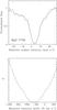 |
Fig. 1 Example of the cross-correlation of two profiles from different exposures. Upper panel: normalized intensities of the Mg ii λ2796 Å line from the zabs = 1.5864 system (Sect. 4.2) extracted from exposure #2, setting 760 (solid line) and from exposure #1, setting 760 (dotted line). See Table 1. Lower panel: the dependence of |

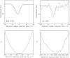 |
Fig. 2 Cross-correlations of profiles from exposures with high signal levels. All lines are from the zabs = 0.45207 system. Left upper panel: solid line – the normalized Mg ii λ2796 Å profile composed from 12 exposures with similar signal levels (100–150 counts per pixel at the continuum level); dotted line – the normalized Mg ii λ2796 Å profile from the exposure #2, setting 437 (Table 1) with a high level of signal (~500 counts per pixel). Left lower panel: |
At first, we calculate the redshift zabs of a given absorption-line system. This redshift is fixed for all other lines from this system. All line position measurements are carried out in the velocity scale. Namely, for each absorption line with the laboratory wavelength λ0, a spectral region centered at λobs = λ0 (1 + zabs) and wide enough to incorporate clear “continuum windows” from both sides (blueward and redward) of λobs is converted into the velocity scale as V = c(λ − λobs)/λobs, where c is the speed of light and λ is the current wavelength. The continuum windows are used to determine the local continuum level and to normalize the extracted line profiles.
As already mentioned above, the profiles from individual exposures may be shifted relative to each other. To evaluate these shifts we used a procedure that cross-correlates two normalized profiles I1 and I2: one of the chosen profiles (I1) is fixed and the other (I2) is moved relative to I1 by a small step, δv (usually δv ≈ 50 m s-1, i.e., of about 0.05 pixel size). At each step, a value of  – the sum of squares of the intensity differences over n pixels covering the line – is calculated,
 ![\hbox{${\cal{S}}(\delta v) = \sum_{j=1}^{n} [I_{1,j} - I_{2,j}(\delta v)]^2$}](/articles/aa/full_html/2011/05/aa16194-10/aa16194-10-eq58.png) . depends parabolically on δv, being minimal when the profiles are aligned. This shift at the minimum of
. depends parabolically on δv, being minimal when the profiles are aligned. This shift at the minimum of  is taken as a local velocity offset, ΔV, between the two profiles. An example of this cross-correlation is shown in Fig. 1.
Cross-correlating the profiles of different lines from different exposures we found that (i) the velocity shifts between individual exposures of the same line were, in general, within | ΔV | ≤ 500 m s-1; (ii) the shift between two arbitrary chosen exposures was not a constant, but varied from line to line (i.e., wavelength dependent). This supports the above statement that calibration accuracy is affected by many factors. Then, a natural solution to obtain the resulting line profile would be to average over all factors, i.e., to sum up all available exposures.
However, a particular feature of the present observations is that because of the seeing conditions, the signal changes significantly between exposures of different settings. Namely, for the setting 390+580, eight exposures were taken, all with a comparable signal level. But for the setting 437+760, only three exposures were obtained, each of which with a signal much higher than in the setting 390+580. The high-signal exposures have larger weights in the sum and, hence, even a single miscalibrated high-signal profile can noticeably shift the combined profile.
To avoid these shifts, we firstly co-added only profiles with a comparable signal and then checked whether the profiles from the high signal exposures – if present – were shifted with respect to this combined profile or not. An example is shown in Fig. 2, left panel. The shifted exposures were aligned with the combined profile and then all available profiles were co-added to provide the final line.
Calculations showed that the alignment of the high signal exposures resulted in a shift of the final line center of about 40 − 50 m s-1 compared to a line obtained by a simple co-adding (i.e., without alignment) of all profiles. This value is of the same order as the statistical errors with which the centers of strong and narrow absorption lines can be measured (see, e.g., Tables 4, 5) and, therefore, the alignment is important while dealing with these lines. In contrast, the centers of weak lines are measured with errors of 100–200 m s-1, which means that the alignment of the high signal exposures does not lead to statistically significant differences. Nevertheless, in the present study the profiles of weak lines were also prepared with the alignment because in many cases this operation allowed us to obtain more regular (smooth) profiles. However, the profiles of weak lines can be severely distorted by noise, which would result in artificially exaggerated ΔV values (Fig. 2, right panel). That is why the exposure shifts were calculated for a strong absorption line located in the vicinity (within 15–20 Å) of a weak line and then applied to the individual profiles of this weak line.
The wavelength range above 7200 Å is covered by the three exposures of the setting 760 (divided into low and upper frames) and by the three exposures of the setting 700 (also low and upper frames), all having significantly different signals. For absorption lines from this range, the individual profiles were aligned with a profile from the exposure with the highest signal. In turn, the local calibration (i.e., at the position of a particular line) of this exposure was checked using different transitions of the same ion (see Sects. 4.2 and 4.4).
The combined profiles were normalized by means of a smoothing spline and then the rms noise was calculated using the continuum windows. These final profiles were fitted to Gaussians defined by the standard parameters: the component center V, the broadening Doppler parameter b, and the column density N. The FWHM values to convolve the synthetic profiles with the spectrograph point-spread function were estimated from the ThAr lines in the vicinity of particular absorption lines. These values range between 4.3 and 5.4 km s-1. However, in some cases a simultaneous fitting of several lines of the same ion shows that the FWHM should be slightly (~5%) lower than the value estimated from the ThAr lines. This can be explained by additional broadening of the ThAr lines caused by the pressure effects since these lines arise in dense plasma.
The errors of the fitting parameters were calculated through the inverse second derivatives matrix. Because we are especially interested in the accurate error of the line center V, this error was additionally evaluated using the Δχ2-method (Press et al. 1992). As the actual error of the line center the higher estimate was accepted.
It is well known that the noise produced by CCDs is highly correlated (e.g., Levshakov et al. 2002). These correlations do not affect the results of the χ2-minimization, but they reduce the apparent dispersion of the noise and consequently lead to the underestimation of the calculated errors of the fitting parameters. In order to understand how to correct the estimated errors, the following Monte-Carlo experiment was performed. First, we synthesized a line profile with a given set of parameters. The spectrum of HE0001–2340 reveals wide continuum windows (e.g., in the range 4474–4692 Å or 5130–5314 Å), which in fact represent long sequences (several thousands of points) of correlated noise values. In these windows, we choose at random a point and starting from it extracted n subsequent values, which were added to the synthesized profile (n is the number of pixels covering the line). Then the profile parameters were evaluated with the standard χ2-minimization. The procedure was repeated 1000 times, and the dispersions of the resulting distributions of the fitting parameters were taken as their errors. They were ≈ 1.5 times larger than the errors estimated with the inverse matrix (or the errors estimated from the Δχ2-procedure with the confidence level of Δχ2 = 1). Thus, the final errors listed in Tables 4–6 below represent the calculated values multiplied by 1.5.
The difference between the radial velocities V1,V2 of two absorption lines can be used to estimate a putative variation of the fine-structure constant α in space and time with respect to its laboratory (terrestrial) value. For two transitions with different sensitivities to α changes the value of Δα/α = (αz − αlab)/αlab is calculated as Δα/α = (V1 − V2)/ [2c(Q2 − Q1)] , where c is the speed of light, and Q1,Q2 are the corresponding sensitivity coefficients (Dzuba et al. 2002; Berengut et al. 2010).
4. Results
4.1. Absorber at zabs = 0.45207
This unique systems exhibiting a set of Fe i lines was discovered and first described by D’Odorico (2007). The system consists of two components separated by ≈ 70 km s-1 (Fig. 3). The red component shows only a strong Mg ii doublet and weak Fe ii λλ2600,2382 Å lines, but the blue component contains, along with Fe i, narrow and well distinguished lines of Mg ii λλ2796,2803 Å, Mg i λ2852 Å, Fe ii λλ2600,2382, 2344,2374 Å, Ca ii λλ3969,3934 Å, and Ca i λ4227 Å with simple profiles and represents in fact the best-choice system to measure the Mg isotope abundance ratio. In the previous spectrum of HE0001–2340 taken with a lower spectral resolution (pixel size ≈ 2.3 km s-1, FWHM = 6.8 km s-1), the Mn triplet λλ2576,2594,2606 Å can be safely identified and probably also a line of Si i λ2515 Å. Unfortunately, in our spectrum, which was obtained with a higher resolution and because of this has a lower S/N, these lines are indistinguishable from noise fluctuations.
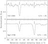 |
Fig. 3 Observed profiles of the Fe ii and Mg ii lines from the zabs = 0.45207 system toward the quasar HE0001–2340. The system consists of two subcomponents separated by ≈ 70 km s-1. The zero radial velocity is fixed at z = 0.45207. Note the difference between relative line intensities in the subcomponents. |
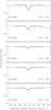 |
Fig. 4 Fe i lines from the zabs = 0.45207 system toward the quasar HE0001–2340 (solid-line histograms). Synthetic profiles are plotted by the smooth curves. The signal-to-noise ratio, S/N, per pixel in the co-added spectrum is indicated in each panel. The zero radial velocity is fixed at z = 0.45207. |
Calculations were performed with the line profiles prepared as described in Sect. 3. Some special cases are outlined below.
Fe i λ2967 Å (Fig. 4). The line is weak and not seen in individual exposures. However, this Fe i transition has the highest sensitivity to changes in α (Dzuba & Flambaum 2008), so it was important to obtain its line profile as accurately as possible. Fortunately, 12 Å redward to the position of Fe i λ2967 (at λ ≈ 4309 Å) lies a strong Al ii λ1670 Å line from the zabs = 1.5864 system (Sect. 4.2), which can be used to calculate the shifts of the individual exposures and to test the local wavelength scale calibration. The corresponding spectral ranges are present in all 14 exposures – the eight exposures of the setting 390 with similar signal, the three high-signal exposures of the setting 437, and the three intermediate-signal exposures of the setting 420. Employing our standard procedure of the line profile preparation, we would sum up the eight equal-signal profiles from the setting 390, align the profiles from the high-signal exposures with this combined profile, and then co-add all available exposures. I.e., the reference for the final profile would be set by the average profile from the setting 390. But the comparison of the Al ii λ1670 Å line produced by the eight co-added exposures of this setting with other low-ionization lines Si ii λ1526 Å and Fe ii λλ2382,2600,2586,2344,2374,1608 Å from the same zabs = 1.5864 system showed that the Al ii profile was shifted relative to these lines by ≈ 0.5 km s-1, whereas the profile composed from the combined six exposures of the settings 437 and 420 was coherent with them. Therefore, in the present case, the reference profile was obtained by co-adding the exposures from settings 437 and 420, and the alignment was performed for the individual Al ii profiles from the setting 390. The same procedure was used to prepare the resulting profile of the Fe i λ2967 Å line: the exposures of the settings 437 and 420 remained unchanged, whereas those from the setting 390 were shifted in accord with the shifts calculated for the Al ii λ1670 Å profiles. Additionally, exposures exhibiting noise spikes within the Fe i λ2967 Å profile were excluded from the final co-adding (three exposures from the setting 390 and three from the setting 420).
Fe i λ3021 Å (Fig. 4). In spite of its weakness, the line is well distinguishable in all available 14 exposures (settings 390, 437, 420). However, from unknown reasons (may be because of the absence of appropriate ThAr lines in the vicinity of λ = 4387 Å where Fe i λ3021 is located) the final profile appeared to be offset relative to the other Fe i lines. However, the sensitivities to α variations of the Fe i λ3021 Å and λ2967 Å transitions are equal, and these lines should be aligned at any rate. The cross-correlation of the Fe i λ3021 Å and λ2967 Å lines showed that the former was shifted by − 0.35 km s-1. The calibration of the Fe i λ2967 Å line was verified by the Al ii λ1670 Å line from the zabs = 1.5867 system, and therefore we aligned the Fe i λ3021 Å line with Fe i λ2967 Å, i.e., shifted it by 0.35 km s-1.
 |
Fig. 5 Same as Fig. 4 but for Fe ii lines. The right panel shows the decomposition of the λ2586 Å line, which is blended with two Ly-α forest absorption lines (see text for details). |
Fe i λ3720 Å (Fig. 4). The line is weak and present only in the eight exposures of the frame 580l. Because of the similar sensitivity to α changes, its position should coincide with the Fe i λ2484 Å and Fe i λ2523 Å lines, but the cross-correlation showed that the Fe i λ3720 Å line was offset by − 0.3 km s-1. In contrast, the profiles of Fe i λλ2484,2523,2967, and 3021 (corrected) were coherent, which means that Fe i λ3720 was affected by some miscalibration. Thus, the final line profile of Fe i λ3720 Å was shifted by 0.3 km s-1.
Fe ii λ2586 Å (Fig 5, right panel). This quite strong line is blended with Ly-α forest absorptions, but can be accurately deconvolved. The noise was calculated as the difference between the observed and the fitted spectrum and added to the deconvolved Fe ii λ2586 Å profile shown in Fig. 5, left panel.
Ca i λ4227 Å (Fig. 6). This weak line is located at λ = 6138 Å. Close to its position, there are a weak Fe ii λ2374 Å (at λ = 6142 Å), and a strong Fe ii λ2382 Å (at λ = 6163 Å) lines, both from the zabs= 1.5864 system. The lines are present in the 14 exposures: eight from the frame 580u, three from 700l, all 11 with a similar signal, and three from the frame 760l with high but different in all three exposures signals. The velocity shifts of the profiles from the frame 760l relative to the co-added 11 profiles from the frames 580u and 720l were calculated for the high-contrast Fe ii λ2382 Å line. Then the same shifts were applied to the Fe ii λ2374 Å exposures from the setting 760l. The final profiles of Fe ii λλ2382,2374 Å were perfectly aligned with the Fe ii λλ2600,2586,1608 Å lines and with other low-ionization lines from the zabs = 1.5864 system. The same procedure was applied to the Ca i line: profiles from the frame 760l were shifted in accord with the Fe ii λ2382 Å exposures and then co-added with unchanged profiles from the frames 580u and 700l.
Mg i λ2852 Å (Fig. 6). The line is weak and located at 4142 Å. Close to its position at 4150 Å, there is a high-contrast line of O i λ1032 Å from the zabs= 2.1871 system (Sect. 4.4). The Mg i profiles from the high-signal exposures (settings 437) were corrected following the shifts of this O i line.
Mg ii λλ2796,2803 Å (Fig. 6). Both lines are strong and present in all 14 exposures. However, the profiles of Mg ii λ2803 Å in four exposures (two of the setting 390, ons of the setting 437, and ons of the setting 420) are severely distorted and not included in the final spectrum. This explains the different S/N ratios for the Mg ii λ2796 Å and Mg ii λ2803 Å lines shown in Fig. 6.
As a result, we have for the analysis the following set of the absorption lines: Mg i λ2852, Mg ii λλ2796,2803, Fe i λλ2484,2523, 2967,3021,3720, Fe ii λλ2600,2382, 2586,2344,2374, Ca i λ4227, and Ca ii λλ3934,3969 Å. The line profiles of each ion were analyzed independently. Trial calculations have shown that a single-component Gaussian profile is sufficient to fit properly all lines. However, the value of χ2 ≲ 1 in the fitting of the Mg ii doublet (highest S/N ratio) could be achieved only with a covering factor  , i.e., assuming an incomplete coverage of the background light source: alternative models with two components and
  yield very small b-parameter ( ≈ 0.5 km s-1), which is inconsistent with the line widths of other species from this system. Spectra of other ions have lower S/N ratios and their fits with and with are statistically indistinguishable, although χ2 in trials with was always lower (e.g., 0.7 vs. 0.9). Thus, the final calculations were performed with for all ions.
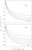 |
Fig. 7 Velocity shift ΔV as function of the ratio ξ = (25Mg+ 26Mg)/24Mg for the Mg i λ2852 Å (upper panel) and the Mg ii λ2796 Å (lower panel) lines. The curves are calculated for different ratios of the heavy isotopes, r = 26Mg/25Mg (depicted over each curve). ΔV = 0 corresponds to the solar value of the Mg isotope ratios, ξ⊙ = 0.2660 and r⊙ ≈ 1. The horizontal dashed lines mark the mean values of ΔVMg I and ΔVMg II measured at zabs = 0.45207, whereas the dotted lines restrict the ± 1σ uncertainty intervals (see text for details). |
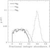 |
Fig. 8 Empirical probability distribution functions (p.d.f.) for Mg isotopic fractional abundances, f, estimated by a Monte Carlo procedure (see Sect. 4.1 for details) |
The covering factor  is easily determined from a slightly modified model of the line profile,
 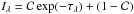 , under the assumption that is the same for the whole absorbing cloud (i.e., it does not depend on λ or, equivalently, on the radial velocity V). Here, I is the observed normalized intensity within the absorption line profile and τλ is the optical depth. The covering factor can differ from ion to ion since, in general, different ions trace different gas. If at least two lines of the same ion are available, then the covering factor is estimated safely. If only one line is present, then the covering factor cannot be determined (degenerate with column density) and has to be fixed to some value (see note to Table 4). Indeed, the incomplete covering is quite common among the so-called associated (i.e. located close to the background quasar) absorbers and not such a rare finding even among intergalactic absorbers (see examples in Paper I). The cause of the light leakage is not clear, but it is probably related to the gravitational lensing of the quasar beam by some intervening galaxy/cluster. In any case we can conclude that the absorber showing the incomplete covering of the background source is to be very small, probably even of a sub-parsec linear size. Note that the incomplete covering in the zabs = 0.45207 system was recently mentioned also by Jones et al. (2010).
The observed and synthetic profiles from the zabs = 0.45207 system are shown in Figs. 4–6, and the corresponding fitting parameters are listed in Table 4.
The radial velocity of the system center calculated as the weighted mean value of the Fe ii, Fe i, Ca ii, and Ca i line centers is Vc = −1.77 ± 0.03 km s-1. Then for the velocity offsets of the Mg lines we obtain the following values: ΔVMg II ≡ VMg II − Vc = −0.44 ± 0.05 km s-1, ΔVMg I ≡ VMg I − Vc = −0.17 ± 0.17 km s-1, i.e., negative velocity shifts are detected for both the Mg ii lines and the Mg i line, although for the latter it is only at the 1σ level because of a large uncertainty of the Mg i line position (weak single line). However, before ascribing this shift to the enhanced content of the heavy Mg isotopes in the absorbing gas, the arguments concerning possible calibration errors and kinematic shifts (the so-called “Doppler noise”) should be considered.
The centers of both Fe ii and Fe i lines are determined from five transitions, and therefore they provide a robust mean radial velocity. The calibration of Ca ii and Ca i lines is verified by the Fe ii λλ2382,2374 Å lines from the zabs = 1.5864 system and their centers coincide with those of the Fe ii and Fe i lines within the 1σ uncertainty interval.
Both Mg ii lines fall in the spectral region with the highest S/N ratio. They are narrow and strong – this explains a small error (0.04 km s-1) of the line center determination. However, the systematic error owing to miscalibration can easily reach the tenfold value as was shown above for, e.g., the Fe i λ3021 Å and Fe i λ3720 Å lines. Can the positions of the Mg ii lines be also affected by some additional errors? The answer is very probable negative. The main factor here is that the position of Mg ii λ2803 coincides with a strong and unsaturated line Th i λ4070 Å from the ThAr spectrum, which is used as a reference for the wavelength calibration. As a result of this coincidence, the Mg ii λ2803 profiles from different exposures are almost aligned (shifts < 0.05 km s-1). Individual profiles of the Mg ii λ2796 reveal shifts up to ± 250 m s-1 (see, e.g., Fig. 2), but the final Mg ii λ2796 profile prepared by the standard procedure (i.e., similar-signal exposures co-added to form a preliminary profile, high-signal exposures aligned with this profile and then all exposures co-added again) is fully coherent with Mg ii λ2803. In general, all lines in the present study that were found to be shifted owing to calibration errors (e.g., Fe i λ3021, this section, Fe ii λ1608 at zabs = 2.1871, Sect. 4.4) fall in the gaps between ThAr reference lines, whereas lines with good calibration (e.g., Si ii λ1526 and Fe ii λ2344 from the zabs = 2.1871 system, Sect. 4.4) coincide with some of the ThAr lines. The conclusion that the vicinity to some of the ThAr reference lines ensures a stable wavelength calibration is further supported by the comparison of the line positions in the archive HE0001–2340 spectrum and in the present one: the “coinciding” lines are coherent in both spectra, whereas centers of lines from the gaps can differ by ~0.5 km s-1. Thus, the negative shift of the Mg ii lines in the system under consideration cannot be caused by calibration errors. The same statement is valid for the Mg i λ2852 line as well, since its position is also close to a ThAr reference.
Neither can this shift be attributed to the gas flows inside the absorber. The estimated Doppler b-parameters (Table 4) show that the line broadening is not thermal and, hence, some turbulent component is present. But the line centers of Fe ii and Fe i (as well as Ca ii and Ca i) coincide within the 1σ uncertainty interval – contrary to the centers of the Mg ii and Mg i lines. However, at values of the ionization parameter log U ≲ − 4, which is the range most probable for the system under study (D’Odorico 2007; Jones et al. 2010), the ionization curves of the Mg ii and Fe ii ions are almost parallel, whereas the ionization curves of Fe i and Fe ii diverge. Thus, for any density/velocity gradients inside the absorbers one would expect rather a shift between the centers of the Fe i and Fe ii lines, but not between Fe ii and Mg ii.
This leaves us the assumption that the measured negative shift of the Mg ii and Mg i lines relative to other lines in the zabs = 0.45207 system is indeed caused by enhanced content of heavy Mg isotopes in the absorbing gas. Figure 7 shows the velocity shift ΔV as a function of the ratio ξ = (25Mg+ 26Mg)/24Mgfor the Mg i λ2852 Å (upper panel) and the Mg ii λ2796 Å (lower panel) lines. The curves are calculated for different ratios of the heavy isotopes, r = 26Mg/25Mg, which are depicted over each curve. The laboratory wavelengths for separate isotopes are taken from Salumbides et al. (2006) and from Batteiger et al. (2009) for, respectively, Mg i and Mg ii. ΔV = 0 corresponds to the solar value of the Mg isotope ratios, ξ⊙ = 0.2660 and r⊙ ≈ 1. The horizontal dashed lines mark the measured mean values of ΔVMg I = −170 m s-1 and ΔVMg II = −440 m s-1, and the dotted lines restrict the ± 1σ uncertainty interval for Mg ii (for Mg i, it runs from ΔVMg I = 0 to − 340 m s-1). From the lower panel of Fig. 7 we immediately see that the measured shift of the Mg ii lines can be produced by the isotope mixture with ξ > 1.5 and r > 1, i.e., with an overabundance of 26Mg relative to other two isotopes.
Using the values of ΔVMg I and ΔVMg II and their errors, we can estimate the most probable fractional abundances f24,f25, and f26 of Mg isotopes assuming that the measured velocity shifts are random values normally distributed with the means − 170 m s-1 and − 440 m s-1 and the dispersions of 170 m s-1 and 50 m s-1, respectively. Figure 8 shows the empirical probability distribution functions for each isotope obtained by Monte-Carlo modeling when ΔVMg I and ΔVMg II were chosen at random from the corresponding normal distributions and f24,f25, and f26 were calculated under the conditions f24 + f25 + f26 = 1, each fk > 0, ξ = (f25 + f26)/f24 > 1.5, and r = f26/f25 > 1. Evidently the abundances of the first two isotopes 24Mg and 25Mg are almost rectangularly distributed, whereas the fractional abundance of 26Mg is distributed normally. The calculated statistics are f24 = 0.19 ± 0.11, f25 = 0.22 ± 0.13, and f26 = 0.59 ± 0.06.
In order to understand what causes the enhanced abundances of the heavy Mg isotope in the zabs = 0.45207 system the origin of this absorber should be clarified. Consider now the column densities of the ions presented in Table 4. Although accurate ionization corrections are not known, we can unambiguously conclude that the relative abundance of iron to magnesium, (Fe/Mg) ≳ 5, is by almost an order of magnitude higher than its solar value, (Fe/Mg)⊙ = 0.83 since the ionization corrections for Fe ii are always higher than that for Mg ii irrespectively of the shape of the ionizing radiation and the value of the ionization parameter U. The ionization curves of magnesium and calcium at log U ≲ − 4 closely trace each other, and from the comparison of the column densities of Mg i and Mg ii with those of Ca i and Ca ii we obtain that the relative content of calcium to magnesium, (Ca/Mg) ≈ 0.4, considerably exceeds its solar value, (Ca/Mg)⊙ = 0.06. As already mentioned above, in the system under study there is probably the Si i λ2515 Å line, but its identification is uncertain since it falls into the Ly-α forest. If the absorption at the expected position of the Si i line is indeed caused by this transition, then N(Si i) = (7.0 ± 0.7) × 1011 cm-2 (D’Odorico 2007). The ionization correction for Si i at log U ≲ − 4 is very close to that for Mg i, and comparing N(Si i) with N(Mg i) we obtain again a significant relative overabundance of silicon to magnesium: (Si/Mg) = 3.7 vs. (Si/Mg)⊙ = 0.98. This abundance pattern – a high iron content, overabundances of Si and Ca relative to Mg – is usually observed in remnants of type Ia supernovae (e.g., Stehle et al. 2005; Mazzali et al. 2008; Tanaka et al. 2010). The Mn ii triplet, although indistinguishable in our data, is clearly visible in the low-resolution spectrum of HE0001–2340, where N(Mn ii) = (3.6 ± 0.4) × 1011 cm-2 was determined by D’Odorico (2007). It is not clear how to translate this column density into the Mn abundance, but taking into account the trace solar content of Mn, (Mn/Fe)⊙ = 0.01, a very high relative abundance and even an overabundance of Mn relative to Fe seems to be quite probable. And this supposes a high metallicity progenitor, since in general the abundance of Mn in the supernova Ia remnants is thought to be correlated with the metallicity (expressed as the initial content of 22Ne) of the exploding white dwarf (McWilliam et al. 2003; Badenes et al. 2008). Model calculations of nucleosynthetic yields from SN Ia do not predict an enhanced content of heavy Mg isotopes for the whole SN Ia remnant, but a very high concentration of 26Mg is predicted for the outer layer of the exploding white dwarf where it is synthesized through alpha-capture on 22Ne (Seitenzahl et al. 2010). The SN remnants are known to be heterogeneous objects displaying complex variations of chemical composition with position and velocity (e.g., Hughes et al. 2000). Indeed, the zabs = 0.45207 system also consists of two separated components (Fig. 3) with obviously different physical parameters. Taking into account the tiny linear size (manifested through the incomplete coverage of the light source) of the analyzed clump at V = 0 km s-1 we can suggest that it is a fragment of a SN Ia remnant.
As already mentioned above, different sensitivity of different Fe i, Fe ii, and Ca ii transitions to changes in the fine-structure constant α makes it possible to estimate Δα/α from the velocity shifts of the corresponding line centers. Unfortunately, the measured errors of the line centers in the present system allow us to put constraints on Δα/α only at the level of 10-5, with the most accurate estimate provided by Fe i lines: Δα/α = (0.6 ± 1.0) × 10-5.
We note that Chand et al. (2004) and Murphy et al. (2008) estimated Δα/α in this system using the Mg ii λλ2796,2803 Å and Mg i λ2852 Å transitions as reference. A negative Δα/α value reported by Murphy et al. is obviously a consequence of the unaccounted Mg isotope shift.
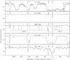 |
Fig. 9 Overview of the H i Ly-α, Fe ii λ2600 Å, Mg ii λ2796 Å, C iv λ1548 Å, and Si iv λ1393 Å profiles from the zabs= 1.5865 absorption complex toward the quasar HE0001–2340. The complex consists of four sub-systems (A,B,C,D) spread over 1100 km s-1. The zero radial velocity is fixed at zA = 1.5864. |
4.2. Absorber at zabs = 1.5864
This system represents a large absorbing complex extending over ~1000 km s-1 (Fig. 9). The redshift z = 1.5864 corresponds to the sub-system A with the strongest low-ionization lines (Fe ii, Si ii, Mg ii, Al ii). The sub-system D at V = −1200 km s-1 was described in Paper I as a high-metallicity absorber enriched by AGB-stars. The sub-systems A and B probably originate in low-ionization clumps (lines of F ii, Mg ii, Si ii, C ii, Al ii) embedded in gas with a higher ionization, which is seen in lines of Si iv and C iv. Note a remarkable kinematic similarity between Mg ii and Fe ii absorptions in these sub-systems and Mg ii and Fe ii absorptions in the previously described system at zabs = 0.45207 (see Fig. 3).
Here we describe the sub-system A in the context of measuring the Mg isotope abundance ratio. Unfortunately, in the sub-system B the Mg ii λλ2796,2803 lines are contaminated with telluric absorptions, which prevent us from accurately measuring their centers. The observed line profiles shown by the histograms in Fig. 10 were prepared as described in Sect. 3. Some particular details are given below.
Fe ii λ2586 Å. Three profiles from the frame 580u are severely corrupted and were excluded from the final co-added spectrum. This explains a lower S/N at the position of this line compared to the neighboring Fe ii λ2600 Å line.
Fe ii λ2600 Å. The cross-correlation of the Fe ii λ2600 Å and Fe ii λ2382 Å profiles revealed a shift of 0.15 km s-1 between them. Because trial fittings of Fe ii lines have shown the consistency of Fe ii λ2382 Å with Fe ii λλ2344,2586,2374, and 1608 Å, the final Fe ii λ2600 Å line was aligned with Fe ii λ2382 Å (i.e., shifted by 0.15 km s-1).
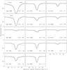 |
Fig. 10 Metal absorption lines from the zabs = 1.5864 system toward the quasar HE0001–2340 (solid-line histograms). Synthetic profiles are plotted by the smooth curves. The signal-to-noise ratio, S/N, per pixel in the co-added spectrum is indicated in each panel. The zero radial velocity is fixed at z = 1.5864. |
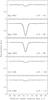 |
Fig. 11 Metal absorption lines from the zabs = 1.6515 system toward the quasar HE0001–2340 (solid-line histograms). Synthetic profiles are plotted by the smooth curves. The signal-to-noise ratio, S/N, per pixel in the co-added spectrum is indicated in each panel. The zero radial velocity is fixed at z = 1.6515. |
Fe ii λ1608 Å. The line is very weak and barely visible in the individual exposures. In the spectrum of HE0001–2340, it lies at 4160 Å – close to a strong O i λ1302 Å line from the zabs = 2.1871 system at 4150 Å (Sect. 4.4). The position of this O i line is verified by comparison with the Si ii λ1260 Å and Si ii λ1526 Å lines from the zabs = 2.1871 system. Thus, the Fe ii λ1608 Å profiles from three exposures of the high-signal setting 437 were shifted in accord with the shifts of the O i λ1302 Å line.
Al ii λ1670 Å. See Sect. 4.1 where Fe i λ2967 Å line is described.
Mg ii λλ2796,2803 Å. Both lines are very strong and present in three exposures of the frame 760l and three exposures of the frame 700u, all having different S/N ratios. The exposure with the highest S/N (#8 from 700u, Table 1) was taken as a reference and all other exposures were aligned with it before co-adding.
Mg i λ2852 Å. The line is very weak and its profiles in the individual exposures (three from 760l and three from 700u) are severely distorted by noise. All available exposures were simply co-added without any preliminary alignments. This means that the final profile is mostly affected by the strongest exposure #8 from 700u.
C ii λ1334 Å. The line is almost saturated, has a low S/N and is partly blended with Ly-α forest absorptions. The line center cannot be estimated with accuracy better than 1 km s-1 and we did not include the C ii λ1334 Å line in the final analysis.
The lines of each ion (Fe ii, Si ii, Al ii, Al iii, Mg ii, Mg i) were fitted independently using Gaussian components. In each case the number of components was determined as a minimum required to fit the profile with χ2 ≲ 1. The fitting parameters are listed in Table 5, the synthetic profiles are shown in Fig. 10 by the solid lines. The weighted value for the system center calculated from the Fe ii, Si ii, and Al ii lines is Vc = 3.54 ± 0.03 km s-1. This gives the offset for the Mg ii line of ΔVMg II ≡ VMg II − Vc = 0.17 ± 0.05 km s-1 and ΔVMg I = 0.04 ± 0.45 km s-1 for Mg i.
As mentioned above, the profiles of the Mg ii lines from individual exposures were aligned with the exposure #8 from the frame 700u having the strongest signal. The offset revealed is the sum of two effects: a shift of the reference exposure, and a shift of the Mg ii lines owing to enhanced content of heavy isotopes. The value of the exposure shift can be estimated from the following consideration. The Mg ii lines are located in the range Δλ = 7230−7252 Å. The frame 700u starts at 7050 Å (Table 2), and up to the positions of the Mg ii lines there are no absorption lines in the spectrum, which can be used to verify the wavelength calibration. However, the frame 760l (another frame whose exposures contribute to the Mg ii profiles) starts at shorter wavelengths (covering Δλ = 5694 − 7532 Å), and up to 6809 Å it overlaps with the wavelength interval covered by the frame 580u. In the range covered by both the 760l and 580u frames there are several absorption lines from three different systems (Ca ii λλ3934,3969 Å, Ca i λ4227 Å at zabs = 0.45207; Fe ii λλ2344,2374,2382,2586,2600 Å from the present system; and Fe ii λ2382 Å at zabs = 1.6515), which can be used to cross-check the calibration of the exposures from the frame 760l. This cross-checking shows that the strongest exposure #3 has a systematic positive shift from 0.3 km s-1 (positions of Ca ii λλ3934,3969 Å, Ca i λ4227 Å at zabs = 0.45207) to 0.2 km s-1 (positions of Fe ii λλ2586,2600 Å from the present system) relative to the center of each absorption-line system. In turn, the Mg ii profiles from the exposure #8 (700u) and #3 (760l) coincide, i.e., at the position of the Mg ii lines these two exposures are coherent. Thus, we can assume that the reference exposure #8 (700u) has a positive shift of ≤ 0.2 km s-1. This gives us a conservative lower limit on the offset of the Mg ii lines due to enhanced content of heavy isotopes of ΔVMg II ≳ −0.08 km s-1. Assuming 26Mg/25Mg > 1, which is supported both by measurements in presolar spinel grains and in some Milky Way giants (Gyngard et al. 2010; Yong et al. 2006) and by theoretical predictions (Karakas et al. 2006), we obtain (25Mg+ 26Mg)/24Mg ≲ 0.7 (see Fig. 7, lower panel). We note that in the previous (lower resolution) spectrum of HE0001–2340 the Mg ii lines from the zabs = 1.5864 system are shifted with respect to the Mg ii lines from the present spectrum by ≈ − 0.5 km s-1.
Again, the presence of spectral lines with different sensitivities to changes in α makes it possible to estimate the value of Δα/α, but now with a considerably higher accuracy because the errors of the line centers are small. Namely, by comparing the Si ii λ1526 Å line as a transition unaffected by α-variations with a sensitivity coefficient Q ≈ 0.001 (Dzuba et al. 2002) with the Fe ii λλ2600,2586,2382,2374,2344 Å transitions, all having similar sensitivity coefficient of Q ≈ 0.04 (Porsev et al. 2007), we obtain Δα/α = (−1.5 ± 2.6) × 10-6. This is comparable with the most stringent constraint on |Δα/α| < 2 ppm found from the Fe ii lines at z = 1.15 toward the bright quasar HE 0515–4414 (Quast et al. 2004; Levshakov et al. 2005, 2006; Molaro et al. 2008b).
The line Fe ii λ1608 Å with Q = −0.016 is very weak and besides its red wing is slightly corrupted by the noise spike (Fig. 10). If only the blue (incorrupted) portion of the Fe ii λ1608 Å profile is taken, then Δα/α estimated from the Fe ii transitions is Δα/α = (−0.5 ± 11.0) × 10-6.
4.3. Absorber at zabs = 1.6515
This system was described in Paper I where the following relative abundances were determined: [C/H] = 0.4 − 0.45, [Mg/C] = 0.1 − 0.15, [Fe/C] ≲ −0.3, and [Si/C] = −0.8. This abundance pattern relates the absorbing gas with the outflows from AGB-stars. A high content of magnesium along with a relative deficit of iron is one of the characteristics of hot-bottom burning (Herwig 2005), which can result in an enhanced content of the neutron-rich Mg isotopes. Indeed, analyzing the previous (lower resolution) spectrum of HE0001–2340, we noticed that Mg ii lines were offset by ≈ − 0.6 km s-1 relative to the lines of other low-ionization species from this system. Here we present accurate line centers based on the higher resolution spectrum.
The available low-ionization transitions are C ii λ1334 Å, Si ii λλ1260, 1526 Å, Fe ii λ2382 Å, Mg ii λλ2796,2803 Å, and Mg i λ2852 Å. However, the C ii λ1334 Å and Si ii λ1260 Å lines are blended with strong Ly-α absorptions and cannot be deconvolved with a sufficiently high accuracy. The combined Mg ii λλ2796,2803 Å profiles consist of six co-added exposures (three from 760l, and three from 700u) aligned with the exposure #8 (700u). The weak Mg i λ2852 Å line is present only in three exposures of the frame 700u, which were simply co-added, i.e., the profile of this line is mostly affected by the exposure #8 with the strongest signal. The profiles of Si ii λ1526 Å and Fe ii λ2382 Å were prepared as described in Sect. 3.
The line centers were determined for the Si ii λ1526 Å, Fe ii λ2382 Å, Mg ii λλ2796,2803 Å, and Mg i λ2852 Å lines. Lines of each ion were fitted independently. The blue wing of Mg ii λ2796 Å is blended with a weak telluric absorption, but the central part of this line is unaffected. The fitting parameters are listed in Table 6, the observed and synthetic profiles are shown in Fig. 11. The system center calculated as the weighted mean between the centers of the Si ii λ1526 Å and Fe ii λ2382 Å lines is Vc = −4.05 ± 0.20 km s-1, which gives the offsets ΔVMg II = −0.08 ± 0.20 km s-1, and ΔVMg I = −0.28 ± 0.44 km s-1.
The Mg ii lines are observed in the range Δλ = 7414 − 7434 Å. At both sides of this region there are absorption lines with verified calibration. Namely, at 7380 Å, the Mg i λ2852 Å line from the zabs = 1.5864 system is present and its position coincides with other lines from this system (Table 4). At 7472 Å, we have the Fe ii λ2344 Å line from the zabs = 2.1871 system, and this line is also unshifted (see Sect. 4.4). Thus, the calibration of the Mg ii lines is correct. As for the Mg i λ2852 Å line, it lies close to the Fe ii λ2374 Å line from the zabs = 2.1871 system, which is shifted relative to Fe ii λ2344 Å by 0.2 km s-1 (Sect. 4.4). Therefore, the Mg i λ2852 Å line is very probably shifted as well, i.e., VMg I should be − 4.13 ± 0.39 km s-1, and ΔVMg I = −0.08 ± 0.44 km s-1. Because of weakness of the Si ii λ1526 Å and Fe ii λ2382 Å lines their positions are measured with large errors, making the shift of Mg lines statistically indistinguishable from zero. Under the assumption that 26Mg/25Mg > 1, a tentative upper limit on (25Mg+ 26Mg)/24Mg is ≲ 2.6.
4.4. Absorber at zabs = 2.1871
This absorber belongs to an extended sub-DLA system described in detail in Richter et al. (2005). It exhibits multiple lines of O i, Si ii, Mg ii, and Fe ii, which can be used to check the calibration uncertainties.
The O i λλ1302, 1039 Å, Si ii λλ1526, 1304, 1260, 1190 Å, Fe ii λλ2600, 2586, 2382, 2374, 2344, 1608 Å, and Mg ii λλ2803, 2796 Å lines are present in many exposures of different settings. Their profiles were prepared as described in Sect. 3.
The Fe ii λλ2586,2600 Å lines are detected in three exposures of the frame 760u and in three exposures of the frame 700u (all exposures with different S/N). Before co-adding, the exposures were aligned with the exposure #3 (760u) showing the highest S/N. We note that Fe ii profiles from this exposure completely coincide with Fe ii profiles from the exposure #8 (700u) which is the highest S/N exposure in the setting 700u.
The Fe ii λ2344 Å line is present in 3 exposures of 760l and in 3 exposures of 700u. Again, all of them have different S/N. The alignment was performed relative to the exposure #8 (700u).
The Fe ii λλ2382,2374 Å lines are present only in 3 exposures of 700u where their profiles are completely consistent, and the final profiles were obtained by simple co-adding.
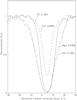 |
Fig. 12 Absorption lines from the zabs = 2.1871 system overlapped to demonstrate different profile shapes. The Fe ii λ2600 Å line is shifted by 0.35 km s-1, and the Mg ii λ2796 Å line by 1.08 km s-1 with respect to their original positions in the spectrum (see Sect. 4.4 for details). The zero radial velocity is fixed at z = 2.1871. |
The Mg ii λλ2796,2803 Å lines are present in 3 exposures of 760u. Before co-adding, individual profiles were aligned with the profile from the exposure #3.
Line profiles of different ions in the zabs = 2.1871 system differ from each other, which is clearly visible in Fig. 12 where several profiles are overplotted. This means that the absorbing gas has density and velocity gradients. However, all ions trace some central condensation, and we can estimate the shifts between the lines of different ions using their central components. Lines of each ion were fitted independently to Gaussians, the number of which was determined as a minimum required to fit all transitions of a given ion with χ2 ≲ 1. The synthetic profiles are shown by solid lines in Fig. 13. The fitting parameters are listed in Table 7. Some details on the fitting procedure are explained below.
The ion O i is represented by the lines 1302 Å and 1039 Å. The O i λ1302 Å line is almost saturated and the 1039 Å line falls in a very noisy part of the spectrum. To constrain the fitting parameters we included in the analysis the O i λ988 Å line from the previously obtained spectrum of HE0001–2340 with FWHM = 6.8 km s-1 (its profile is also shown in Fig. 13).
Trial fittings of Si ii lines showed that the Si ii λ1190 Å line was noticeably shifted with respect to the Si ii λλ1260, 1526,1304 Å lines and that the synthetic Si ii λ1304 Å line came out systematically weaker than the observed one (see Fig. 13). Both the 1190 Å and 1304 Å lines were excluded from the fitting procedure, and the fitting parameters were estimated on the base of the 1260 Å and 1526 Å lines. After the fitting procedure, the synthetic profile of the 1190 Å line was calculated and the shift of the observed 1190 Å line was evaluated by cross-correlation of the synthetic and observed profiles. We found that Si ii λ1190 Å line was shifted by − 0.6 km s-1 relative to the other Si ii transitions. This line is located just at the order edge, which probably explains the revealed discrepancy. As for the Si ii λ1304 Å line, the reason for its intensity to be underestimated whereas the profiles of the Si ii λ1260, 1190 (shifted), and 1526 Å lines are fitted perfectly, is unclear. May be it is because of a blend with some unidentified absorption.
Trial fittings of the available Fe ii lines (λλ2600,2586, 2374,2382,2344,1608 Å) revealed that all of them are shifted with respect to each other. We are especially interested in calibration of the Fe ii λ2344 Å line since it lies in the vicinity of the Mg ii doublet from the zabs = 1.6515 system (Sect. 4.3) and can be used to verify its position. We took Fe ii λ2344 Å as a reference line, calculated offsets for the other Fe ii lines, and aligned all profiles. Then the aligned Fe ii lines were fitted together. The fitting parameters and the shifts of the individual lines relative to Fe ii λ2344 Å are shown in Table 7. The center of the 2344 Å line coincides within the uncertainty interval with the centers of the O i and Si ii lines. Thus, we can conclude that the exposure #8 from the frame 700u (reference exposure for the alignment of the individual Fe ii λ2344 Å profiles before co-adding) at 7472 Å (position of Fe ii λ2344 Å) has no offsets relative to the zero-point. Note that there is a good ThAr reference line at 7472 Å. However, negative offsets begin to appear at larger wavelengths being − 0.2 km s-1 at 7564 Å (Fe ii λ2374 Å), − 0.25 km s-1 at 7594 Å (Fe ii λ2382 Å), − 0.45 km s-1 at 8244 Å (Fe ii λ2586 Å), and − 0.35 km s-1 at 8286 Å (Fe ii λ2600 Å).
 |
Fig. 13 Metal absorption lines from the zabs = 2.1871 system toward the quasar HE0001–2340 (solid-line histograms). Synthetic profiles are plotted by the smooth curves. The signal-to-noise ratio, S/N, per pixel in the co-added spectrum is indicated in each panel. Also shown are the relative velocity offsets ΔV: for the Si ii λ1190 Å line and the Mg ii doublet they are with respect to the Si ii λλ1260,1526 Å lines, and for the Fe ii lines – relative to the Fe ii λ2344 Å line. The zero radial velocity is fixed at z = 2.1871. |
A negative offset is clearly displayed also by the Mg ii λλ2796,2803 Å doublet located in the range 8912 − 8936 Å: it is shifted by − 1.08 ± 0.13 km s-1 relative to Si ii lines (Table 7). To what extent this offset is caused by a putative high content of heavy Mg isotopes is not clear. According to Richter et al. (2005), in the present system [O ] = −1.8 and [N/O ] < −1.5, i.e., enrichment occurred because of metal-poor SN II. Thus, from general considerations the enhanced ratio (25Mg+ 26Mg)/24Mg should not be expected. It is likely that the shift of the Mg ii lines is mostly caused by the distortions in the calibration process.
This tendency – increasing negative offsets with increasing wavelength in the range λ > 7500 Å – is detected not only in the present spectrum, but in other UVES spectra as well. Such offsets are found both in the archive QSO spectra and in spectra newly obtained within the framework of the ESO Large Program 185.A-0745. At the hardware level the UVES is realized by the two arms – blue and red, and in the red one there are two CCD chips – lower (REDL) and upper (REDU). The blue arm covers the range 3000–5000 Å, and the red arm 4200 − 11 000 Å. The performance of the blue and lower red chips was checked by an original procedure involving solar radiation reflected by asteroids (Molaro et al. 2008a) and no large systematic shifts in the wavelength calibration between two chips were detected. Our data support this result, although they also demonstrate that local line position shifts with amplitudes in most cases below |ΔV| = 0.4 km s-1 (<1/3 pixel size) are possible. Why the wavelength calibration slides down in spectra detected with the REDU chip (7500 Å < λ < 9000 Å) is unclear and this problem needs a thorough investigation. In any case, obviously that the studies involving differential measurements of the line positions may use REDU spectra only if there are some independent methods to check their wavelength calibration.
This is just the case of the system considered here where calibration of Fe ii λ2344 Å is verified by comparison with multiple lines of other ions (O i and Si ii). Since the sensitivity coefficients of O i is QO I ≈ 0 (Berengut & Flambaum 2010) and of Si ii is QSi II ≈ 0.001 (Dzuba et al. 2002), positions of the O i and Si ii lines should not be affected by putative variations of the fine-structure constant α, whereas the sensitivity coefficient of the Fe ii λ2344 Å transition is 0.036 (Porsev et al. 2007). The difference ΔV between the Fe ii λ2344 Å and O i/Si ii line centers is much smaller than the error of ΔV, which is 0.11 km s-1 if the O i line center is taken as a zero-point, and 0.13 km s-1 if Si ii is a reference line. The former case gives us the value Δα/α = (1.4 ± 5.1) × 10-6, the latter – Δα/α = (−0.9 ± 6.0) × 10-6. In turn, the line Fe ii λ1608 Å with Q = −0.016 is shifted by 0.3 km s-1 relative to the Fe ii λ2344 Å, which would give us the value Δα/α = (9.6 ± 4.5) × 10-6. This example confirms the conclusion of Griest et al. (2010) that calibration errors are the main source of uncertainties in Δα/α estimations from absorption lines in quasar spectra.
We note that the present system was used by Chand et al. (2004) and by Murphy et al. (2008) to estimate Δα/α from the transitions Mg ii λ2803 Å, Al ii λ1670 Å, Si ii λ1526 Å, and Fe ii λλ2374,2586 Å, which were fitted simultaneously using the same model. It is unclear how this could be done taking into account that in the previous HE0001–2340 spectrum all peculiarities described above (e.g., extreme shift of the Mg ii lines and different line profiles of different ions) were also present.
5. Conclusions
We attempted to measure the Mg isotope abundances in several absorption systems detected in the spectrum of the quasar HE0001–2340. The spectrum was obtained with the VLT/UVES with the slit width of 0.7 arcsec and was read pixel by pixel without binning, thus ensuring a pixel size about twice as small as was achieved in previous (archived) spectra of this source (1.3 km s-1 vs. 2.3 km s-1). The line profiles were individually prepared according to a special procedure described in Sect. 3. Absorption-line systems selected for the study reveal multiple lines of the same ions (e.g., Si ii λλ1526,1304,1260 Å, Fe ii λλ2382,2374,2344 Å etc.), which can be used to verify the local wavelength calibration. The main results are the following.
-
1.
For the first time we measured the abundance of Mg isotopes in the high-redshift absorber at zabs = 0.45207, which is probably a remnant of the SN Ia explosion of high-metallicity white dwarf(s). Lines of the Mg ii doublet are shifted relative to low-ionization transitions of other ions (Fe i, Fe ii, Ca i, Ca ii) by ΔVMg II = −0.44 ± 0.05 km s-1, and the Mg i line by ΔVMg I = −0.17 ± 0.17 km s-1. This translates into the isotope abundance ratio 24Mg:25Mg:26Mg = (19 ± 11):(22 ± 13):(59 ± 6) with a strong relative overabundance of heavy Mg isotopes 25Mg+26Mg relative to 24Mg compared to the solar ratio 24Mg:25Mg:26Mg = 79:10:11.
-
2.
In the absorbers at zabs = 1.5864 and zabs = 1.6515 arising in the gas enriched likely by outflows from AGB type stars we obtain for the shift of the Mg ii lines relative to other ions the values of ΔVMg II ≳ − 0.08 km s-1 at zabs = 1.5864, and ΔVMg II = −0.08 ± 0.20 km s-1 at zabs = 1.6515. This allows us to set only upper limits on the content of heavy Mg isotopes in the absorbing gas: (25Mg+ 26Mg)/24Mg ≲ 0.7 at zabs = 1.5864, and (25Mg+ 26Mg)/24Mg ≲ 2.6 at zabs = 1.6515.
-
3.
In the present spectrum of HE0001–2340 the errors of the wavelength calibration produce velocity shifts of absorption lines with amplitudes in most cases below 0.4 km s-1 (1/3 pixel size). This statement is valid for the wavelength ranges covered by the blue and REDL chips of the UVES. However, absorption lines taken with the REDU chip are systematically shifted toward shorter wavelengths. The discrepancy increases with increasing wavelength and may reach − 1 km s-1 ( ≈ 0.8 pixel size) in the wavelength interval 7500 Å < λ < 9000 Å.
-
4.
In the absorption system at zabs = 1.5864 with the verified calibration of the metal absorption lines, we set a limit on the variation of the fine-structure constant at the level of Δα/α = (−1.5 ± 2.6) × 10-6, which is one of the most stringent estimates of this value obtained from optical spectra of QSOs.
-
5.
Comparison of statistical errors of the line position measurements with systematic errors owing to miscalibration of the wavelength scale shows that the systematic error is the main source of uncertainties in the measurements of Δα/α from quasar absorption-line systems.
Online material
Journal of the observations.
Wavelength ranges covered by individual settings.
Atomic data for Mg i, Mg ii, Al ii, Al iii, Si ii, Ca i, Ca ii, Fe i, and Fe ii resonance transitions.
Fitting parameters of spectral lines identified in the zabs = 0.45207 absorber.
Fitting parameters of spectral lines identified in the zabs = 1.5864 absorber.
Fitting parameters of the spectral lines identified in the zabs = 1.6515 absorber.
Fitting parameters of the spectral lines identified in the zabs = 2.1871 absorber.
Acknowledgments
The project has been supported in part by the RFBR grants 09-02-12223 and 09-02-00352, by the Federal Agency for Science and Innovations grant NSh-3769.2010.2, and by the Chinese Academy of Sciences visiting professorship for senior international scientists grant No. 2009J2-6. H.J.L. is supported by the NSF of China Key Project No. 10833005, the Group Innovation Project No. 10821302, and by 973 program No. 2007CB815402.
References
- Aldenius, M. 2009, Phys. Scr., 134, 014008 [NASA ADS] [CrossRef] [Google Scholar]
- Ashenfelter, T. P., Mathews, G. J., & Olive, K. A. 2004, ApJ, 615, 82 [NASA ADS] [CrossRef] [Google Scholar]
- Badenes, C., Bravo, E., & Hughes, J. P. 2008, ApJ, 680, L33 [NASA ADS] [CrossRef] [Google Scholar]
- Batteiger, V., Knünz, S., Herrmann, M., et al. 2009, Phys. Rev. A, 80, 022503 [NASA ADS] [CrossRef] [Google Scholar]
- Berengut, J. C., & Flambaum, V. V. 2010, Hyperfine Interact., 196, 269 [NASA ADS] [CrossRef] [Google Scholar]
- Berengut, J. C., Dzuba, V. A., Flambaum, V. V., et al. 2010 [arXiv:1011.4136] [Google Scholar]
- Chand, H., Srianand, R., Petitjean, P., & Aracil, B. 2004, A&A, 417, 853 [NASA ADS] [CrossRef] [EDP Sciences] [Google Scholar]
- Centurión, M., Molaro, P., & Levshakov, S. 2009, MmSAIt, 80, 929 [NASA ADS] [Google Scholar]
- D’Odorico, V. 2007, A&A, 470, 523 [NASA ADS] [CrossRef] [EDP Sciences] [Google Scholar]
- Dzuba, V. A., & Flambaum, V. V. 2008, Phys. Rev. A, 77, 012514 [NASA ADS] [CrossRef] [Google Scholar]
- Dzuba, V. A., Flambaum, V. V., Kozlov, M. G., & Marchenko, M. 2002, Phys. Rev. A, 66, 022501 [NASA ADS] [CrossRef] [Google Scholar]
- Edlén, B. 1966, Metrologia, 2, 71 [NASA ADS] [CrossRef] [Google Scholar]
- Griest, K., Whitmore, J. B., Wolfe, A. M., et al. 2010, ApJ, 708, 158 [NASA ADS] [CrossRef] [Google Scholar]
- Gyngard, F., Zinner, E., Nittler, L. R., et al. 2010, ApJ, 717, 107 [NASA ADS] [CrossRef] [Google Scholar]
- Hughes, J. P., Rakowski, C. E., Burrows, D. N., & Slane, P. O. 2000, ApJ, 528, L109 [NASA ADS] [CrossRef] [PubMed] [Google Scholar]
- Jones, T. M., Misawa, T., Charlton, J. C., Mshar, A. C., & Ferland, G. J. 2010, ApJ, 715, 1497 [NASA ADS] [CrossRef] [Google Scholar]
- José, J., Coc, A., & Hernanz, M. 1999, ApJ, 520, 347 [NASA ADS] [CrossRef] [Google Scholar]
- José, J., Hernanz, M., Amari, S., Lodders, K., & Zinner, E. 2004, ApJ, 612, 414 [NASA ADS] [CrossRef] [Google Scholar]
- Karakas, A. I. 2010, MNRAS, 403, 1413 [NASA ADS] [CrossRef] [Google Scholar]
- Karakas, A. I., & Lattanzio, J. C. 2003, Publ. Astron. Soc. Australia, 20, 279 [CrossRef] [Google Scholar]
- Karakas, A. I., Lugaro, M. A., Wiescher, M., Görres, J., & Ugalde, C. 2006, ApJ, 643, 471 [NASA ADS] [CrossRef] [Google Scholar]
- Kaufer, A., D’Odorico, S., & Kaper, L. 2004, UV-Visual Echelle Spectrograph. User Manual, http://www.eso.org/instruments/uves/userman/ [Google Scholar]
- Larson, J. M., & Modigliani, A. 2009, UVES Pipeline User Manual http://www.eso.org/sci/facilities/paranal/instruments/uves/doc/index.html [Google Scholar]
- Levshakov, S. A. 1994, MNRAS, 269, 339 [NASA ADS] [Google Scholar]
- Levshakov, S. A., Dessauges-Zavadsky, M., D’Odorico, S., & Molaro, P. 2002, ApJ, 565, 696 [NASA ADS] [CrossRef] [Google Scholar]
- Levshakov, S. A., Centurión, M., Molaro, P., & D’Odorico, S. 2005, A&A, 434, 827 [NASA ADS] [CrossRef] [EDP Sciences] [Google Scholar]
- Levshakov, S. A., Centurión, M., Molaro, P., et al. 2006, A&A, 449, 879 [NASA ADS] [CrossRef] [EDP Sciences] [Google Scholar]
- Levshakov, S. A., Agafonova, I. I., Molaro, P., Reimers, D., & Hou, J. L. 2009, A&A, 507, 209 [Paper I] [NASA ADS] [CrossRef] [EDP Sciences] [Google Scholar]
- Lodders, K., Palme, H., & Gail, H.-P. 2009, Abundances of the elements in the Solar System, ed. J. E. Trümper, SpringerMaterials – The Landolt-Börnstein Database (Berlin Heidelberg: Springer-Verlag) [arXiv:astro-ph/0901.1149] [Google Scholar]
- Mazzali, P. A., Sauer, D. N., Pastorello, A., Benetti, S., & Hillebrandt, W. 2008, MNRAS, 386, 1897 [NASA ADS] [CrossRef] [Google Scholar]
- McWilliam, A., Rich, R. M., & Smecker-Hane, T. A. 2003, ApJ, 592, L21 [NASA ADS] [CrossRef] [Google Scholar]
- Molaro, P., Levshakov, S. A., Monai, S., et al. 2008a, A&A, 481, 559 [NASA ADS] [CrossRef] [EDP Sciences] [Google Scholar]
- Molaro, P., Reimers, D., Agafonova, I. I., & Levshakov, S. A. 2008b, EPJST, 163, 173 [Google Scholar]
- Morton, D. C. 2003, ApJS, 149, 205 [NASA ADS] [CrossRef] [MathSciNet] [Google Scholar]
- Murphy, M. T., Webb, J. K., Flambaum, V. V., et al. 2001, MNRAS, 327, 1208 [NASA ADS] [CrossRef] [Google Scholar]
- Murphy, M. T., Webb, J. K., & Flambaum, V. V. 2008, MNRAS, 384, 1053 [NASA ADS] [CrossRef] [Google Scholar]
- Nave, G., & Sansonetti, C. J. 2010, private communication [Google Scholar]
- Porsev, S. G., Koshelev, K. V., Tupitsyn, I. I., et al. 2007, Phys. Rev. A, 76, 052507 [NASA ADS] [CrossRef] [Google Scholar]
- Press, W. H., Teukolsky, S. A., Vetterling, W. T., & Flannery, B. P. 1992, Numerical Recipes in C (Cambridge: Cambridge Uni. Press) [Google Scholar]
- Quast, R., Reimers, D., & Levshakov, S. A. 2004, A&A, 415, L7 [NASA ADS] [CrossRef] [EDP Sciences] [Google Scholar]
- Reimers, D., Köhler, T., & Wisotzki, L. 1996, A&AS, 115, 235 [NASA ADS] [Google Scholar]
- Richter, P., Ledoux, C., Petitjean, P., & Bergeron, J. 2005, A&A, 440, 819 [NASA ADS] [CrossRef] [EDP Sciences] [Google Scholar]
- Salumbides, E. J., Hannemann, S., Eikema, K. S. E., & Ubachs, W. 2006, MNRAS, 373, L41 [NASA ADS] [Google Scholar]
- Sarazin, M., & Roddier, F. 1990, A&A, 227, 294 [NASA ADS] [Google Scholar]
- Seitenzahl, I. R., Röpke, F. K., Fink, M., & Pakmor, R. 2010, MNRAS, 407, 2297 [NASA ADS] [CrossRef] [Google Scholar]
- Stehle, M., Mazzali, P. A., Benetti, S., & Hillebrandt, W. 2005, MNRAS, 360, 1231 [NASA ADS] [CrossRef] [Google Scholar]
- Tanaka, M., Mazzali, P. A., Stanishev, V., et al. 2011, MNRAS, 410, 1725 [NASA ADS] [CrossRef] [Google Scholar]
- Uzan, J.-P. 2010, [arXiv:1009.5514] [Google Scholar]
- Whitmore, J. B., Murphy, M. T., & Griest, K. 2010, ApJ, 723, 89 [NASA ADS] [CrossRef] [Google Scholar]
- Wisotzki, L., Köhler, T., Groote, D., & Reimers, D. 1996, A&AS, 115, 227 [NASA ADS] [Google Scholar]
- Wisotzki, L., Christlieb, N., Bade, N., et al. 2000, A&A, 358, 77 [NASA ADS] [Google Scholar]
- Yong, D., Lambert, D. L., & Ivans, I. I. 2003, ApJ, 599, 1357 [NASA ADS] [CrossRef] [Google Scholar]
- Yong, D., Aoki, W., & Lambert, D. L. 2006, 638, 1018 [Google Scholar]
- Zinner, E., Nittler, L. R., Hoppe, P., et al. 2005, Geochim. Cosmochim. Acta, 69, 4149 [NASA ADS] [CrossRef] [Google Scholar]
All Tables
Atomic data for Mg i, Mg ii, Al ii, Al iii, Si ii, Ca i, Ca ii, Fe i, and Fe ii resonance transitions.
Fitting parameters of the spectral lines identified in the zabs = 1.6515 absorber.
Fitting parameters of the spectral lines identified in the zabs = 2.1871 absorber.
All Figures
|
Fig. 1 Example of the cross-correlation of two profiles from different exposures. Upper panel: normalized intensities of the Mg ii λ2796 Å line from the zabs = 1.5864 system (Sect. 4.2) extracted from exposure #2, setting 760 (solid line) and from exposure #1, setting 760 (dotted line). See Table 1. Lower panel: the dependence of |
| In the text | |
|
Fig. 2 Cross-correlations of profiles from exposures with high signal levels. All lines are from the zabs = 0.45207 system. Left upper panel: solid line – the normalized Mg ii λ2796 Å profile composed from 12 exposures with similar signal levels (100–150 counts per pixel at the continuum level); dotted line – the normalized Mg ii λ2796 Å profile from the exposure #2, setting 437 (Table 1) with a high level of signal (~500 counts per pixel). Left lower panel: |
| In the text | |
|
Fig. 3 Observed profiles of the Fe ii and Mg ii lines from the zabs = 0.45207 system toward the quasar HE0001–2340. The system consists of two subcomponents separated by ≈ 70 km s-1. The zero radial velocity is fixed at z = 0.45207. Note the difference between relative line intensities in the subcomponents. |
| In the text | |
|
Fig. 4 Fe i lines from the zabs = 0.45207 system toward the quasar HE0001–2340 (solid-line histograms). Synthetic profiles are plotted by the smooth curves. The signal-to-noise ratio, S/N, per pixel in the co-added spectrum is indicated in each panel. The zero radial velocity is fixed at z = 0.45207. |
| In the text | |
|
Fig. 5 Same as Fig. 4 but for Fe ii lines. The right panel shows the decomposition of the λ2586 Å line, which is blended with two Ly-α forest absorption lines (see text for details). |
| In the text | |
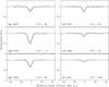 |
Fig. 6 Same as Fig. 4 but for the Mg i, Mg ii, Ca i, and Ca ii lines. |
| In the text | |
|
Fig. 7 Velocity shift ΔV as function of the ratio ξ = (25Mg+ 26Mg)/24Mg for the Mg i λ2852 Å (upper panel) and the Mg ii λ2796 Å (lower panel) lines. The curves are calculated for different ratios of the heavy isotopes, r = 26Mg/25Mg (depicted over each curve). ΔV = 0 corresponds to the solar value of the Mg isotope ratios, ξ⊙ = 0.2660 and r⊙ ≈ 1. The horizontal dashed lines mark the mean values of ΔVMg I and ΔVMg II measured at zabs = 0.45207, whereas the dotted lines restrict the ± 1σ uncertainty intervals (see text for details). |
| In the text | |
|
Fig. 8 Empirical probability distribution functions (p.d.f.) for Mg isotopic fractional abundances, f, estimated by a Monte Carlo procedure (see Sect. 4.1 for details) |
| In the text | |
|
Fig. 9 Overview of the H i Ly-α, Fe ii λ2600 Å, Mg ii λ2796 Å, C iv λ1548 Å, and Si iv λ1393 Å profiles from the zabs= 1.5865 absorption complex toward the quasar HE0001–2340. The complex consists of four sub-systems (A,B,C,D) spread over 1100 km s-1. The zero radial velocity is fixed at zA = 1.5864. |
| In the text | |
|
Fig. 10 Metal absorption lines from the zabs = 1.5864 system toward the quasar HE0001–2340 (solid-line histograms). Synthetic profiles are plotted by the smooth curves. The signal-to-noise ratio, S/N, per pixel in the co-added spectrum is indicated in each panel. The zero radial velocity is fixed at z = 1.5864. |
| In the text | |
|
Fig. 11 Metal absorption lines from the zabs = 1.6515 system toward the quasar HE0001–2340 (solid-line histograms). Synthetic profiles are plotted by the smooth curves. The signal-to-noise ratio, S/N, per pixel in the co-added spectrum is indicated in each panel. The zero radial velocity is fixed at z = 1.6515. |
| In the text | |
|
Fig. 12 Absorption lines from the zabs = 2.1871 system overlapped to demonstrate different profile shapes. The Fe ii λ2600 Å line is shifted by 0.35 km s-1, and the Mg ii λ2796 Å line by 1.08 km s-1 with respect to their original positions in the spectrum (see Sect. 4.4 for details). The zero radial velocity is fixed at z = 2.1871. |
| In the text | |
|
Fig. 13 Metal absorption lines from the zabs = 2.1871 system toward the quasar HE0001–2340 (solid-line histograms). Synthetic profiles are plotted by the smooth curves. The signal-to-noise ratio, S/N, per pixel in the co-added spectrum is indicated in each panel. Also shown are the relative velocity offsets ΔV: for the Si ii λ1190 Å line and the Mg ii doublet they are with respect to the Si ii λλ1260,1526 Å lines, and for the Fe ii lines – relative to the Fe ii λ2344 Å line. The zero radial velocity is fixed at z = 2.1871. |
| In the text | |
Current usage metrics show cumulative count of Article Views (full-text article views including HTML views, PDF and ePub downloads, according to the available data) and Abstracts Views on Vision4Press platform.
Data correspond to usage on the plateform after 2015. The current usage metrics is available 48-96 hours after online publication and is updated daily on week days.
Initial download of the metrics may take a while.