| Issue |
A&A
Volume 529, May 2011
|
|
|---|---|---|
| Article Number | A80 | |
| Number of page(s) | 7 | |
| Section | Planets and planetary systems | |
| DOI | https://doi.org/10.1051/0004-6361/201016162 | |
| Published online | 07 April 2011 | |
HST/STIS Lyman-α observations of the quiet M dwarf GJ 436
Predictions for the exospheric transit signature of the hot Neptune GJ 436b⋆
1
Institut de planétologie et d’astrophysique de Grenoble (IPAG), Université
Joseph Fourier-Grenoble 1, CNRS (UMR 5274), BP 53
38041, Grenoble Cedex 9
France
e-mail: This email address is being protected from spambots. You need JavaScript enabled to view it.
2
Institut d’astrophysique de Paris, Université Pierre et Marie
Curie, CNRS (UMR 7095), 98bis
boulevard Arago, 75014
Paris,
France
Received:
17
November
2010
Accepted:
4
February
2011
Abstract
Lyman-α (Lyα) emission of neutral hydrogen (λ1215.67 Å) is the main contributor to the ultraviolet flux of low-mass stars such as M dwarfs. It is also the main light source used in studies of the evaporating upper atmospheres of transiting extrasolar planets with ultraviolet transmission spectroscopy. However, there are very few observations of the Lyα emissions of quiet M dwarfs, and none exist for those hosting exoplanets. Here, we present Lyα observations of the hot-Neptune host star GJ 436 with the Hubble Space Telescope Imaging Spectrograph (HST/STIS). We detect bright emission in the first resolved and high quality spectrum of a quiet M dwarf at Lyα. Using an energy diagram for exoplanets and an N-body particle simulation, this detection enables the possible exospheric signature of the hot Neptune to be estimated as a ~11% absorption in the Lyα stellar emission, for a typical mass-loss rate of 1010 g s-1. The atmosphere of the planet GJ 436b is found to be stable to evaporation, and should be readily observable with HST. We also derive a correlation between X-ray and Lyα emissions for M dwarfs. This correlation will be useful for predicting the evaporation signatures of planets transiting other quiet M dwarfs.
Key words: ultraviolet: planetary systems / planets and satellites: individual: GJ 436b / planets and satellites: atmospheres / stars: low-mass / stars: activity / techniques: spectroscopic
Based on observations made with the Space Telescope Imaging Spectrograph on board the Hubble Space Telescope (Cycle 17 program GO/DD 11817).
© ESO, 2011
1. Introduction
Planetary transits provide golden opportunities to probe the atmospheres of extrasolar planets. The atmospheric signals detected by this method in the visible (e.g., Charbonneau et al. 2002) are usually tenuous, while the infrared detections of atmospheric signatures remain disputed (e.g., Gibson et al. 2011). In the ultraviolet (UV), planetary transits of the hot giant planet HD 209458b are detected from conspicuous spectroscopic signatures, which are seen as absorption in the emission lines originating from the stellar chromosphere and transition region between the chromosphere and the corona (see Ehrenreich 2010, for a review). The strongest signature is a (15 ± 4)% absorption in the resolved stellar Lyman-α (Lyα) emission line of neutral atomic hydrogen (H i) detected in medium-resolution spectra taken with the Space Telescope Imaging Spectrograph (STIS) on the Hubble Space Telescope (HST) (Vidal-Madjar et al. 2003; see also Ehrenreich et al. 2008). Linsky et al. (2010) present new observations with the Cosmic Origins Spectrograph (COS) on HST. They report a (7.8 ± 1.3)% absorption in the C ii line, confirming the previous result of Vidal-Madjar et al. (2004).
These distinctive UV signatures, compared to those for the visible transit of the whole planet (1.6%; Charbonneau et al. 2000; Henry et al. 2000), require the presence of an extended H i upper atmosphere, or exosphere, to the planet. This envelope must be evaporating because (i) it must fill the planetary Roche lobe to account for the size of the absorption; and (ii) the H i atoms must be accelerated by the stellar radiation pressure beyond the escape velocity of the planet to account for the absorption in the wings of the Lyα line (Vidal-Madjar et al. 2003). The presence of elements heavier than hydrogen (C, O, Si) at high altitudes requires an hydrodynamic escape (or blow-off) of the upper atmosphere, with the flow of escaping H i carrying heavier species up to the Roche limit (Vidal-Madjar et al. 2004; Linsky et al. 2010), where they are swept away by radiation pressure (Lecavelier des Etangs et al. 2008).
New cases of atmospheric escape have been recently reported for two hot jupiters. Lecavelier des Etangs et al. (2010) used HST/ACS to detect the H i exosphere of HD 189733b at Lyα. Fossati et al. (2010) observed the highly irradiated planet host star WASP-12 with HST/COS. They interpret the tentative detection of extra absorption in the metal lines of the star WASP-12 during the transit as signs of mass loss. Thus, atmospheric evaporation could be a common phenonemon among close-in planets.
These results have inspired a comprehensive modelling effort (e.g., García-Muñoz 2007) suggesting that the upper atmospheres of close-in giant planets must be heated by the stellar X-rays, and both extreme and far UV (Cecchi-Pestellini et al. 2009) to about 10 000 K. This temperature has been inferred in the thermosphere of HD 209458b from the detection of excited hydrogen atoms (Ballester et al. 2007). The typical atmospheric mass-loss rate ṁ derived from models is between 1010 and 1011 g s-1. In this case, evaporation should not severely impact the stability of giant planets’ atmospheres. On the other hand, it might be more important for lower-mass planets such as hot Neptunes and super-earths, if their mass-loss rates are of the same order as for more massive planets.
In this article, we evaluate whether mass loss from a hot Neptune such as GJ 436b could be detected with current instrumentation, and what its UV transit signature could be. GJ 436b is the first transiting Neptune-mass planet discovered (Butler et al. 2004). It orbits a close-by (10.2 pc) M2.5v dwarf with V = 10.68, and triggered unprecedented interest when Gillon et al. (2007a) detected a photometric transit of the planet, inferring a true mass of 23.17 M⊕ and a radius of 4.22 R⊕, which are similar to those of either Uranus or Neptune. (The planet properties, taken from Torres 2007, are summarized in Table 1 along with some stellar parameters.) However, GJ 436b differs significantly from the Solar System ice giants because of its moderately eccentric orbit with a semi-major axis of 0.029 astronomical unit (au). At this distance from its 0.026-L⊙ parent star, the planet indeed receives ~30 000 times more flux than Neptune receives from the Sun, and has a blackbody brightness temperature of TB = 717 ± 35 K (Demory et al. 2007). Using the Spitzer Space Telescope, Gillon et al. (2007b) inferred a planet mean density of ~1.7 g cm-3, too weak to be that of a body composed exclusively of water ice, so that GJ 436b must possess a hydrogen/helium envelope that would account for ~10% to 20% of the planet’s mass (Fortney et al. 2007; Figueira et al. 2009). The detection of this envelope with transmission spectroscopy could validate the internal structure models predicting its presence.
To assess this possiblity, it is necessary to derived both the stellar Lyα emission line profile and brightness. We present in Sect. 2 the observations that allowed us to calculate the stellar emission as seen from Earth. We had to correct for the interstellar medium (ISM) absorption before estimating the intrinsic stellar Lyα brightness: this analysis is presented in Sect. 3. In Sect. 4, we estimate a range of plausible mass-loss rates in GJ 436b’s upper atmosphere. This range serves as an input to an atmospheric escape model used to estimate the transit signature of the evaporating hydrogen envelope of the planet in the UV (Sect. 5). To our knowledge, these observations are the first resolved accurate measurement of a quiet M dwarf’s Lyα emission. Hence, we discuss in Sect. 6 how they compare to archival Lyα observations of active M dwarfs.
2. Observations and data reduction
We obtained HST time (GO/DD#11817) to precisely estimate the Lyα emission of the M dwarf GJ 436. The data were recorded on 2010 January 6 with the STIS instrument (Woodgate et al. 1997). The observation consists of one 1762-s exposure on the Far Ultraviolet Multi-Anode Microchannel Array detector (FUV-MAMA). The STIS/FUV-MAMA is a solar-blind cesium iodide (CsI) detector with a 25″ × 25″ field of view (~ pixel-1), operating from 1150 to 1700 Å. The light was diffracted using the long slit of size
  and the first-order grating G140M. This grating was tilted to ensure a central wavelength of 1222 Å. In this configuration, our data have a spectral coverage of 1194–1249 Å with a medium resolution of ~10 000 (30 km s-1) and a throughput of between ~1.2% and 2% (see Proffitt et al. 2010). The data were recorded in time-tag mode, and treated with the version 2.27 of CALSTIS, the STIS data pipeline. CALSTIS performs all the standard data reduction tasks (such as bias and dark subtraction, flat fielding, and wavelength and flux calibrations; see Dressel et al. 2007, for more details). For spectroscopy, the pipeline end-products for a single exposure are the two-dimensional spectral image and the one-dimensional spectrum.
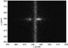 |
Fig. 1 Two-dimensional spectral image of GJ 436. The light is dispersed along the x-axis (roughly). The stellar Lyα emission is seen on both sides of the geocoronal emission, which impacts the detector across the whole y-axis. |
Figure 1 shows the geometrically rectified, wavelength-, and flux-calibrated 2D spectral image (X2D). The spectral dispersion is along the x-axis. In this image, the stellar Lyα emission appears on both sides of the prominent geocoronal emission, which is imaged across the whole detector y-axis. This terrestrial air glow seriously degrades the quality of spectroscopic observations at Lyα; however its rather narrow extent along the dispersion (x-)axis and its large spatial extent (y-axis) enable us to perform an efficient correction. This task is handled by the pipeline subroutine called BACKCORR, which performs the 1D spectral background subtraction. The background is determined along a five-pixel-wide region located ±300 pixels away from the centre of the spectral extraction region. The 1D extracted background is then fitted by a nth degree polynomial, which replaces the background except in the regions surrounding the Lyα line (Dressel et al. 2007). The resulting calibrated 1D spectrum of GJ 436 (X1D) is shown in Fig. 2.
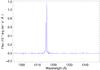 |
Fig. 2 The reduced and calibrated STIS/G140M spectrum of GJ 436 in January 2010. |
3. Lyman-α emission of GJ 436
3.1. Observed flux at Earth
Figure 3 shows a zoomed region of the recorded spectrum around the Lyα line. The error bar for each spectral bin is estimated by CALSTIS, which basically propagates the statistical noise  in each pixel of the raw data, where N is the number of data events (counts) and g is the gain (equal to 1 photon count-1 for MAMA observations).
The total flux of the line seen by HST, integrated from 1 214.40 to 1215.58 Å and from 1215.75 to 1 217.00 Å in order to avoid any residuals from the air glow subtraction at the centre of the line, is (5.490 ± 0.184) × 10-14 erg s-1 cm-2. We note that, as seen from the Earth, the Lyα flux of GJ 436 is higher than that of HD 209458b: the stellar emission from the latter star is also reproduced in Fig. 3 for comparison.
The observed shape of the line is a characteristic double peak resulting from the addition of several profiles, as shown in Fig. 4. As for the Sun (Woods et al. 2005), the core of the intrinsic stellar Lyα line is an emission feature originating in the transition region, where the temperature increases quickly between the chromosphere and the corona. The wings of the Lyα line originate in a deeper chromospheric region. The emission can be either single-peaked or double-peaked, with a central dip due to the high opacity of the abundant hydrogen atoms. As seen from the Solar System, the central part of the line is strongly absorbed by the ISM from 1215.58 to 1215.75 Å. The ISM absorption can indeed be Doppler-shifted relative to the line centre by several kilometers per second. The ISM absorption is the combination of absorption by neutral hydrogen (H i) and deuterium (D i). Deuterium produces narrow absorption at 1215.3 Å, which is blue-shifted by ~0.3 Å from the H i absorption line. The observed Lyα profile is therefore caused by the stellar emission line being absorbed by the ISM and subsequently convolved with the instrumental line spread function (Fig. 4).
3.2. Reconstructed stellar intrinsic emission
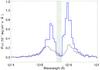 |
Fig. 3 Zoom on the Lyα line of GJ 436 measured with STIS/G140M with error bars from the STIS pipeline (blue curve). The STIS spectrum of HD 209458 obtained by Vidal-Madjar et al. (2003) is shown for comparison (grey curve). As seen from Earth, the nearby M dwarf clearly shows a more intense stellar emission and a narrower ISM absorption. The location of the air glow (subtracted here) is indicated by green hatches. |
To model the hydrogen atom dynamics under the stellar Lyα radiation pressure, we need to estimate the stellar emission line as seen by hydrogen atoms escaping from the planet. To calculate the resulting Lyα transit light curve, we also need to estimate the absorption by the escaping atoms over the stellar profile as seen from the Earth (Sect. 5). To produce these two line profiles, we fitted the observed Lyα profile with a stellar emission line and an ISM absorption model, following the method proposed by Wood et al. (2005). In the following, we assume a D/H ratio of 1.5 × 10⁻⁵. There is widespread consensus (e.g., Ferlet et al. 2000; Hébrard & Moos 2003; Linsky et al. 2006) that this value of the D/H ratio is constant within the Local Bubble (<100 pc; see Wood et al. 2005, and references therein).
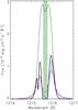 |
Fig. 4 Plot of the theoretical profile of GJ 436’s Lyα line. The black thin line shows the intrinsic stellar emission line as seen by hydrogen atoms escaping the planetary atmosphere. The black thick line shows the resulting profile after absorption by the ISM hydrogen and deuterium. The line profile convolved with the HST G140M instrumental line spread function (red line) is compared to the observations (blue histogram), yielding a good fit with a χ2 of 34.5 for 39 degrees of freedom. The location of the (subtracted) air glow is indicated by green hatches. |
The ISM column density value is chosen within the range considered by Wood et al. (2005), 17.6 < log N(H i) < 18.2. The value is adjusted to 1018 cm-2 using the D i line at 1215.25 Å. This agrees with the ISM column density of log N(H i) = 17.82 measured by Wood et al. (2005) toward the star HD 4345, in a similar direction (11.1° from GJ 436) and at a distance of 21.7 pc. A column density log N(H i) ≫ 18 would be unrealistic for a target as close as GJ 436 (10.2 pc) and yield a stronger D i absorption than observed. (The presence of this feature can be guessed in the blue part of the observed H i Lyα emission in Fig. 3.) In any case, the fit to the observed Lyα profile does not depend much on the assumed ISM column density between N(H i) ~ 1017 and 1018 cm-2 because at these column densities, the H i absorption line is saturated. The result is more dependent on the assumed profile of the wings extrapolated to the core of the emission line.
As pointed out by Wood et al. (2005), the reconstruction of the intrinsic Lyα emission of a star can be affected by absorption from both the heliosphere and the astrosphere, which we did not model for GJ 436. Owing to the moderate resolution of the present observations and our lack of knowledge about the ISM absorption, from either D i or heavier elements (Fe ii or Mg ii), this absorption remain unconstrained. However, GJ 436 is located 87.7° from the upwind direction of the ISM flow seen by the Sun, hence based in Fig. 13 in Wood et al. (2005) it is unlikely that heliospheric absorption is detectable. No extra H i absorption is required besides the ISM component to achieve a good fit of the Lyα line. In particular, we did not consider an astrospheric absorption component. Wood et al. (2005) found that this absorption was necessary in some case to obtain satisfactory fits to the Lyα lines. This does not seem to be the case for GJ 436 given the current data resolution.
We performed the model fitting using several intrinsic line profiles, including a single-peak Gaussian and a double-peaked line modelled by a double Gaussian. We found that the double-peaked Gaussian reproduces far more accurately the observed wings in the line profile. The model intrinsic profile is composed of two Gaussians with the same full width at half maximum (FWHM = Δλ) and line centres separated by the same value, Δλ, which is taken as a free parameter. The line total flux is the second free parameter. The ISM and the stellar radial velocities are also free parameters. The model is convolved with the G140M instrumental line spread function, and compared to the observations. We found a satisfactory fit with Δλ = 0.41 Å, an ISM radial velocity of −4 km s-1 in the stellar reference frame, and a stellar radial velocity corresponding to a Doppler shift of 0.003 Å (~0.7 km s-1). The resulting χ2 is 34.5 for 39 degrees of freedom (see the data and fit in Fig. 4).
The total flux in the reconstructed Lyα line is (2.7 ± 0.7) × 10-13 erg s-1 cm-2. The error bars were estimated by exploring the parameter space for the fit to the observed H i line wings, and considering possible single-peaked profiles or the possibility of two narrow peaks with a deep self-absorption in the central part of the emission line. These last two cases produce extreme Lyα emission profiles within the ISM absorbed wavelength range; the resulting error bars should be considered as conservative.
4. Mass-loss rate of GJ 436b
The mass-loss rate ṁ of GJ 436b is a free parameter in our modelling of the evaporation signature described in the next section. Nevertheless, estimating its value is useful to constraining all the parameter space. To achieve this, we use the method presented by Lecavelier des Etangs (2007), which consists of locating the planet in an “energy diagram”. The energy diagram of exoplanets measures the whole gravitational potential energy of a planet, as a function of high-energy irradiations it receives. This diagram was updated by Davis & Wheatley (2009), and is being completed with a larger sample of transiting planets (Ehrenreich & Désert 2011), including GJ 436.
The resulting diagram is presented in Fig. 5. For GJ 436, we calculate, following Lecavelier des Etangs (2007), the potential energy per mass unit of the planet  (1)where G is the gravitational constant and δtides is the modification of the planet gravitational potential by the stellar tides (see Appendix B of Lecavelier des Etangs 2007).
The energy received by unit of time by GJ 436b can be expressed as  (2)The “X/EUV” in LX/EUV means that the luminosity should be integrated from ~1 Å to 912 Å, following Cecchi-Pestellini et al. (2009).1 However, observations do not usually cover a sufficiently wide bandpass to yield a precise value of LX/EUV. The Rosat luminosity (Hünsch et al. 1999) given in Table 1 is calculated from 0.1 to 2.4 keV, i.e., from 5 to 124 Å. It is, therefore, a lower limit to the actual X/EUV luminosity.
The factor η is the heating efficiency in the exoplanet thermosphere. Lecavelier des Etangs (2007) considered the extreme case of η = 1 where all the stellar flux is used to escape the atmosphere. Considering (without quantifying) energetic losses due to thermal emission by atmospheric hydrogen, Tian et al. (2005) modelled the atmospheric escape process of the hot Jupiter HD 209458b by assuming that η = 0.15. This value was initially chosen by Watson et al. (1981) in their pioneering study of Earth’s atmospheric escape. In the following, we consider both of these values of η.
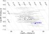 |
Fig. 5 Energy diagram for 100 transiting exoplanets, updated from Lecavelier des Etangs (2007). The energy needed to escape a unit of mass of the planet atmosphere is plotted versus the X/EUV flux. The dotted lines indicate constant mass-loss rates. The blue dot indicates the location of GJ 436b, calculated here assuming an heating efficiency of η = 0.15. The horizontal error bars represent variations in η of between 0.01 and 1. |
Properties of GJ 436 and its planet.
The resulting mass-loss rate is thus  (3)For η = 1 and 0.15, we find that ṁ = 1.07 × 10¹⁰ and 1.60 × 10⁹ g s-1, respectively. These values are close to the canonical escape rate predicted by several evaporation models (e.g., Yelle 2004, 2006; Lecavelier des Etangs et al. 2004; García-Muñoz 2007; Murray-Clay et al. 2009).
5. Observable signature of the evaporating atmosphere
To calculate a theoretical H i transit light curve for various atmospheric escape rates, we modelled the atmospheric gas escaping GJ 436b with a numerical simulation including the dynamics of the hydrogen atoms. In this N-body simulation, hydrogen atoms are released from GJ 436b’s upper atmosphere as particles with a random initial velocity corresponding to a 10 000-K exobase. This temperature corresponds to the temperature expected in the upper atmospheres of hot jupiters (e.g., Lecavelier des Etangs et al. 2004; Stone & Proga 2009) and was inferred from observations (Ballester et al. 2007; Vidal-Madjar et al. 2011). In any case, our results do not depend on this assumption because atoms are rapidly accelerated by the radiation pressure to velocities several times higher than their initial velocities. In this model, the gravity of both the star and the planet are taken into account. The radiation pressure from the stellar Lyα emission line is calculated as a function of the radial velocity of the atoms. The self-extinction within the cloud is also taken into account. The hydrogen atoms are supposed to be ionized by the stellar EUV flux (<912 Å). In the simulation, their lifetime is calculated as a function of the ionizing EUV flux which is taken to be equal to the solar value. The only free parameter is the atomic hydrogen escape rate, expressed in grams per second. The dynamical model provides a steady state distribution of positions and velocities of escaping hydrogen atoms in the cloud surrounding GJ 436b. From this information, we calculated the corresponding absorption over the stellar line (Fig. 6) and the corresponding transit light curve of the total Lyα line (Fig. 7). We found that escape rates of ~109 to 1010 g s-1 can produce absorptions of between ~3% and 11% in the Lyα transit light curve when integrating over the whole line. Absorption depths this large could be promptly detected with HST Lyα observations.
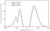 |
Fig. 6 The GJ 436 Lyα spectrum during the transit of GJ 436b. The star spectrum before or after the transit is shown by a thick grey line. The spectrum resulting from the absorption by the planetary exophere during the transit is shown for various escape rates. The blue dotted, the red dot-dashed, and black long-dashed lines show the resulting spectrum when the escape rate is 108, 109, and 1010 g s-1, respectively. With this last escape rate, the blue side of the line is absorbed by about 17%, resulting in a decrease of about 11% in the total Lyman-α flux. |
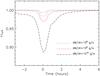 |
Fig. 7 Plot of the theoretical light curve of the total Lyα flux for various escape rates ṁ: 108 g s-1 (blue dotted line), 109 g s-1 (red dot-dashed line), and 1010 g s-1 (black dashed line). The thin long-dashed line shows the light curve for the planet without additional absorption by the planetary atmosphere. |
This contrasts with the atmospheric signatures expected in the infrared. The atmospheric scale height of this planet is H = kBTB/(μgp) ≈ 232 km, where μ = 2 g mol-1 is the molar mass of a H2 atmosphere and gp is the surface gravity of the planet. We can expect atmospheric transit signatures at the level of ~2(ΔF/F)(H/Rp) (Winn 2010), where ΔF/F ≈ (Rp/R⋆)2 ≈ 0.7% is the transit occultation. This yields a typical extra absorption value of ~10-4 for one atmospheric scale height. This value is consistent with the upper limits on the atmospheric absorption of GJ 436b set by Pont et al. (2009), who have covered two near-infrared transits of the planet with the NICMOS camera on HST using a grism to sample the 1.1–1.9 μm band. These authors report observing a flat transmission spectrum at the level of ~10-4, and in particular no significant signal in the 1.4-μm water band (see also Gibson et al. 2011).
Using eclipses of the planet by the star observed by Spitzer, Stevenson et al. (2010) obtained planet-to-star flux ratios that show marginal variations between 3.6 and 24 μm (see also Beaulieu et al. 2011). The interpretation of these broad-band spectrophotometry data is difficult and relies on statistical approaches (Madhusudhan & Seager 2011). Shabram et al. (2011) modelled the infrared transmission spectrum of GJ 436b. These authors conclude that the detailed infrared characterization of this planet may be possible using the James Webb Space Telescope. Before its launch, the use of UV facilities should be considered as a powerful way of characterizing the upper atmospheres of low-mass exoplanets.
6. Lyα emission of M dwarfs and stellar activity
Stellar Lyα emission lines are important spectral features in the context of exoplanet stellar environment and stellar physics. These emission lines are the main contributors to the flux of low-mass stars at short wavelengths, from X to FUV. For instance, the Lyα emission of the Sun contributes to more than 50% of its flux below 1216 Å (Woods et al. 1998). The Lyα line is used as a proxy for determining the temperature and pressure profiles of upper stellar atmospheres.
The Lyα emission originate in the transition regions between the chromospheres and coronae, while other commonly used activity diagnostics are based on indicators originating from the coronae (X-ray flux) or the chromospheres (Mg ii h and k lines). In this context, stellar Lyα emission provides an almost unique access to the structure of the transition region, where the temperature profile exhibits a deep minimum. Houdebine & Doyle (1994) modelled the Lyα emission of M dwarfs. According to their work, the transition region of these stars is thinner than that of solar-like stars.
Stellar Lyα measurements are scarce in the literature. This is mainly because it is impossible to observe this emission from the ground and that it is difficult to correct measurements for the effects of the ISM absorption, both astrospheric and heliospheric absorption, and geocoronal emission. Furthermore, correlations between Lyα emission and other proxies of stellar activity can be misleading because they do not originate in the same region. This ensures that an accurate estimate of the Lyα brightness from an activity relation is rather hazardous. In addition, the Lyα line is extremely variable with time. For the Sun, the integrated Lyα line flux may change by 37% during one rotation and up to 50% over a couple of years (Vidal-Madjar 1975). During the magnetic cycle, the extreme (single day) values can vary by more than a factor of two (Woods et al. 2000).
Very few M dwarfs have Lyα measurements. Landsman & Simon (1993) used the International Ultraviolet Explorer (IUE) to report Lyα fluxes corrected from the ISM absorption for 12 M dwarfs. Wood et al. (2005) obtained resolved Lyα measurements for four M dwarfs with HST/STIS. Three objects are common to both samples, leading to a total of 13 measurements. This sample consists mostly of active stars. In particular, all the HST measurements of Wood et al. (2005) were obtained for M dwarfs with magnetic activity levels well above that of GJ 436. Therefore, our measurement of GJ 436’s Lyα flux is invaluable for estimating the properties of the transition region in quiet M dwarfs.
The measurements found in the literature are listed in Table 2. In Fig. 8, we have plotted the normalized Lyα flux, RLyα = fLyα/fbol as a function of the normalized X-ray flux RX = fX/fbol for the IUE and HST measurements from Table 2. We have not included the available data for YY Gemini and DT Virginis because these stars are close binaries for which a definitive identification of each component’s flux is difficult. The values are listed in Table 2. The observed X-ray fluxes fX are extracted from the Rosat all-sky survey (RASS) in the Nexxus 2 database (Schmitt & Liefke 2004). The bolometric fluxes fbol are obtained by combining the IK photometry of Leggett (1992) with the bolometric correction BCK versus I − K relation of Leggett et al. (2000).
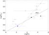 |
Fig. 8 Normalized Lyα flux RLyα = fLyα/fbol as a function of normalized X-ray flux RX = fX/fbol for all the IUE (⋄) and HST (•) Lyα flux measurements of M dwarfs in the literature. Our measurement for GJ 436 data is shown in blue. The dotted lines link HST and IUE mesasurements for objects that have been measured with both instruments. The plain line show the best-fit linear regression to HST measurements, log (RLyα) ≈ 0.5log (RX) − 2.2. The grey dashed line indicates the log RLyα = log RX relation. The horizontal error bars in the X-ray flux are the dispersions reported in Table 2. |
Normalized Lyα and X-ray fluxes of M dwarfs.
As can be seen in Fig. 8, the Lyα fluxes extracted from HST are significantly lower – for a given RX – than those from IUE. Wood et al. (2005) note that the HST and IUE data are coherent for the majority of the objects (besides M dwarfs), except for the fainter ones for which the IUE fluxes are systematically higher than the HST ones. They attribute this to a bias in the corrections for the ISM absorption and geocoronal emission, which are particularly difficult at the lower resolution of IUE.
In the case of faint M dwarfs, we prefer to consider the clearly resolved HST measurements, which were obtained mainly for magnetically active stars. The values of RLyα seem to be correlated to RX for M dwarfs, with log RLyα ≈ 0.5log RX − 2.2, although additional measurements are necessary to confirm this trend. The trend implies that RLya/RX > 1 for quiet M dwarfs, in contrast to the results for more active ones. Figure 8 can thus be used – with caution – to estimate RLyα for all M dwarfs that have values of RX between −5 and −3, i.e., covering the domain of magnetic activity between 20% of that of the quietest M dwarfs in the solar neighbourhood to the very active stars close to the X-ray emission saturation level (see for instance Fig. 5 in Delfosse et al. 1998).
Meanwhile, we stress that the X-ray and Lyα fluxes have been measured here at different times and, therefore, for different magnetic states of the stars, which can add dispersion to any relationship. For GJ 436, the measured log LX ranges from 25.96, as measured with XMM-Newton by Sanz-Forcada et al. (2010), to 27.15, as found in the Rosat/PSPC archives by Poppenhaeger et al. (2010). The value we have used throughout this work comes from the Rosat all-sky survey catalogue of the nearby stars (Hunsch et al. 1999) and is in-between these extreme values. The dispersion (standard deviation) in these three values is σLX = 0.77.
We have retrieved all available X-ray measurements for the stars in Table 2 from the Nexxus 2 database and calculated their σLX. However, these calculated dispersions only provide a rough idea of the real intrinsic X-ray variabilities of the listed M dwarfs, because the number of measurements (also reported in Table 2) is not equivalent for all stars. In addition, the measurements are derived using different instruments, mainly Rosat or XMM-Newton (or both). Differences between surveys, e.g. in the bandpasses, are not taken into account, thus adding to the dispersion. Finally, the occurrence of a flare during a given observation cannot be excluded, leading to a non-Gaussian distribution of the measurements. Therefore, these values should only be regarded as indicative.
7. Conclusion
We have obtained the first UV glance at a star hosting a transiting hot Neptune. The HST data unambiguously show that the early and quiet M dwarf GJ 436 has bright Lyα emission. With an escape rate of around ~1010 g s-1, the hydrogen upper atmosphere of GJ 436b should cause large absorption (~11%) in the Lyα transit light curve. These figures will allow the existence of such an extended upper atmosphere to be tested with a dedicated HST program. These results also suggest that other quiet M dwarfs are brighter at Lyα than in X-rays. This prediction opens new perspectives for the atmospheric characterization of other hot-Neptune and even super-earth atmospheres. Interestingly, the nature of GJ 1214b, a super-earth, or “small-Neptune” also orbiting a quiet M dwarf (Charbonneau et al. 2009), could be resolved with this technique, provided the star is bright enough at Lyα.
In this paper, we use the following conventions for naming spectral regions: X-rays (X) in 1–10 Å, soft X-rays (XUV) in 10–30 Å, extreme ultraviolet (EUV) in 30–912 Å, and far ultraviolet (FUV) in 912–1216 Å.
Acknowledgments
We are particularly grateful to J.-M. Désert and A. Vidal-Madjar for their precious help with the preparation of the HST observations and comments on the manuscript. We thank the anonymous referee for a helpful review. We would also like to thank X. Bonfils, R. Ferlet, T. Forveille, G. Hébrard, A.-M. Lagrange, N. Meunier, and D. K. Sing for stimulating discussions. We also thank M. Mountain for awarding us HST DD time that made this work possible. D.E. is supported by the Centre National d’Études Spatiales (CNES).
References
- Ballester, G. E., Sing, D. K., & Herbert, F. 2007, Nature, 445, 511 [NASA ADS] [CrossRef] [Google Scholar]
- Beaulieu, J.-P., Tinetti, G., Kipping, D. M., et al. 2011, ApJ, 731, 16 [NASA ADS] [CrossRef] [Google Scholar]
- Butler, R. P., Vogt, S. S., Marcy, G. W., et al. 2004, ApJ, 617, 580 [NASA ADS] [CrossRef] [Google Scholar]
- Cecchi-Pestellini, C., Ciaravella, A., Micela, G., & Penz, T. 2009, A&A, 496, 863 [NASA ADS] [CrossRef] [EDP Sciences] [Google Scholar]
- Charbonneau, D., Brown, T. M., Latham, D. W., & Mayor, M. 2000, ApJ, 529, L45 [NASA ADS] [CrossRef] [PubMed] [Google Scholar]
- Charbonneau, D., Brown, T. M., Noyes, R. W., & Gilliland, R. L. 2002, ApJ, 568, 377 [NASA ADS] [CrossRef] [Google Scholar]
- Charbonneau, D., Berta, Z. K., Irwin, J., et al. 2009, Nature, 462, 891 [NASA ADS] [CrossRef] [PubMed] [Google Scholar]
- Davis, T. A., & Wheatley, P. J. 2009, MNRAS, 396, 1012 [NASA ADS] [CrossRef] [Google Scholar]
- Delfosse, X., Forveille, T., Perrier, C., & Mayor, M. 1998, A&A, 331, 581 [NASA ADS] [Google Scholar]
- Demory, B.-O., Gillon, M., Barman, T., et al. 2007, A&A, 475, 1125 [NASA ADS] [CrossRef] [EDP Sciences] [Google Scholar]
- Dressel, L., et al. 2007, STIS Data Handbook, Version 5.0 (Baltimore: STScI) [Google Scholar]
- Ehrenreich, D. 2010, in Physics and Astrophysics of Planetary Systems, ed. T. Montmerle, D. Ehrenreich, & A.-M. Lagrange, EAS Pub. Ser., 41, 429 [Google Scholar]
- Ehrenreich, D., & Désert, J.-M. 2011, A&A, in press [arXiv:1103.0011] [Google Scholar]
- Ehrenreich, D., Lecavelier des Etangs, A., Hébrard, G., et al. 2008, A&A, 483, 933 [NASA ADS] [CrossRef] [EDP Sciences] [Google Scholar]
- Ferlet, R. D., André, M., Hébrard, G., et al. 2000, ApJ, 538, L69 [NASA ADS] [CrossRef] [Google Scholar]
- Figueira, P., Pont, F., Mordasini, C., et al. 2009, A&A, 493, 671 [NASA ADS] [CrossRef] [EDP Sciences] [Google Scholar]
- Fortney, J. J., Marley, M. S., & Barnes, J. W. 2007, ApJ, 659, 1661 [NASA ADS] [CrossRef] [Google Scholar]
- Fossati, L., Haswell, C. A., Froning, C. S., et al. 2010, ApJ, 714, L222 [NASA ADS] [CrossRef] [Google Scholar]
- García-Muñoz, A. 2007, Planet. Space Sci., 55, 1426 [NASA ADS] [CrossRef] [Google Scholar]
- Gibson, N. P., Pont, F., & Aigrain, S. 2011, MNRAS, 411, 2199 [NASA ADS] [CrossRef] [Google Scholar]
- Gillon, M., Pont, F., Demory, B.-O., et al. 2007a, A&A, 472, L13 [NASA ADS] [CrossRef] [EDP Sciences] [Google Scholar]
- Gillon, M., Demory, B.-O., Barman, T., et al. 2007b, A&A, 471, L51 [NASA ADS] [CrossRef] [EDP Sciences] [Google Scholar]
- Hébrard, G., & Moos, H. W. 2003, ApJ, 599, 297 [NASA ADS] [CrossRef] [Google Scholar]
- Henry, G. W., Marcy, G. W., Butler, R. P., & Vogt, S. S. 2000, ApJ, 529, L41 [NASA ADS] [CrossRef] [PubMed] [Google Scholar]
- Houdebine, E. R., & Doyle, J. G. 1994, A&A, 289, 169 [NASA ADS] [Google Scholar]
- Hünsch, M., Schmitt, J. H. M. M., Sterzik, M. F., & Voges, W. 1999, A&AS, 135, 319 [Google Scholar]
- Landsman, W., & Simon, T. 1993, ApJ, 408, 305 [NASA ADS] [CrossRef] [Google Scholar]
- Lecavelier des Etangs, A. 2007, A&A, 461, 1185 [NASA ADS] [CrossRef] [EDP Sciences] [Google Scholar]
- Lecavelier des Etangs, A., Vidal-Madjar, A., McConnell, J. C., & Hébrard, G. 2004, A&A, 418, L1 [NASA ADS] [CrossRef] [EDP Sciences] [Google Scholar]
- Lecavelier des Etangs, A., Vidal-Madjar, A., & Désert, J.-M. 2008, Nature, 456, E1 [NASA ADS] [CrossRef] [PubMed] [Google Scholar]
- Lecavelier des Etangs, A., Ehrenreich, D., Vidal-Madjar, A., et al. 2010, A&A, 514, A72 [NASA ADS] [CrossRef] [EDP Sciences] [Google Scholar]
- Leggett, S. K. 1992, ApJS, 82, 351 [NASA ADS] [CrossRef] [Google Scholar]
- Leggett, S. K., Allard, F., Dahn, C., et al. 2000, ApJ, 535, 965 [NASA ADS] [CrossRef] [Google Scholar]
- Linsky, J. L., Draine, B. T., Moos, H. W., et al. 2006, ApJ, 647, 1106 [NASA ADS] [CrossRef] [Google Scholar]
- Linsky, J. L., Yang, H., France, K., et al. 2010, ApJ, 717, 1291 [NASA ADS] [CrossRef] [Google Scholar]
- Madhusudhan, N., & Seager, S., 2011, ApJ, 729, 41 [NASA ADS] [CrossRef] [Google Scholar]
- Murray-Clay, R. A., Chiang, E. I., & Murray, N. 2009, ApJ, 693, 23 [Google Scholar]
- Perryman, M. A. C., Lindegren, L., Kovalevsky, J., et al. 1997, A&A, 323, L49 [NASA ADS] [Google Scholar]
- Poppenhaeger, K., Robrade, J., & Schmitt, J. H. M. M. 2010, A&A, 515, A98 [NASA ADS] [CrossRef] [EDP Sciences] [Google Scholar]
- Pont, F., Gilliland, R. L., Knutson, H., Holman, M., & Charbonneau, D. 2009, MNRAS, 393, L6 [NASA ADS] [CrossRef] [Google Scholar]
- Proffitt, C., et al. 2010, STIS instrument handbook, Version 9.0 (Baltimore: STScI) [Google Scholar]
- Sanz-Forcada, J., Ribas, I., Micela, G., et al. 2010, A&A, 511, L8 [NASA ADS] [CrossRef] [EDP Sciences] [Google Scholar]
- Schmitt, J. H. M. M., & Liefke, C. 2004, A&A, 417, 651 [NASA ADS] [CrossRef] [EDP Sciences] [Google Scholar]
- Shabram, M., Fortney, J. J., Greene, T. P., & Freedman, R. S. 2011, ApJ, 727, 65 [NASA ADS] [CrossRef] [Google Scholar]
- Stevenson, K. B., Harrington, J., Nymeyer, S., et al. 2010, Nature, 464, 1161 [NASA ADS] [CrossRef] [PubMed] [Google Scholar]
- Stone, J. M., & Proga, D. 2009, ApJ, 694, 205 [NASA ADS] [CrossRef] [Google Scholar]
- Torres, G. 2007, ApJ, 671, L65 [NASA ADS] [CrossRef] [Google Scholar]
- Tian, F., Toon, O. B., Pavlov, A. A., & De Sterck, H. 2005, ApJ, 621, 1049 [NASA ADS] [CrossRef] [Google Scholar]
- Vidal-Madjar, A. 1975, Sol. Phys., 40, 69 [NASA ADS] [CrossRef] [Google Scholar]
- Vidal-Madjar, A., Lecavelier des Etangs, A., Désert, J.-M., et al. 2003, Nature, 422, 143 [NASA ADS] [CrossRef] [PubMed] [Google Scholar]
- Vidal-Madjar, A., Désert, J.-M., Lecavelier des Etangs, A., et al. 2004, ApJ, 604, L69 [NASA ADS] [CrossRef] [Google Scholar]
- Vidal-Madjar, A., Sing, D. K., Lecavelier des Etangs, A., et al. 2011, A&A, 727, A110 [Google Scholar]
- Watson, A. J., Donahue, T. M., & Walker, J. C. G. 1981, 48, 150 [Google Scholar]
- Winn, J. 2010, Transits and Occultations, In Exoplanets, ed. S. Seager (Tucson: University of Arizona Press), in press [Google Scholar]
- Wood, B. E., Redfield, S., Linsky, J. L., Müller, H.-R., & Zank, G. P. 2005, ApJS, 159, 118 [NASA ADS] [CrossRef] [Google Scholar]
- Woods, T. E., Rottman, G. J., Bailey, S. M., & Solomon, S. C. 1998, Sol. Phys., 177, 133 [NASA ADS] [CrossRef] [Google Scholar]
- Woods, T. E., Tobiska, W. K., Rottman, G. J., & Worden, J. R. 2000, J. Geophys. Res., 105, 27195 [NASA ADS] [CrossRef] [Google Scholar]
- Woods, T. E., Eparvier, F. G., Bailey, S. M., et al. 2005, J. Geophys. Res., 110, A01312 [NASA ADS] [CrossRef] [Google Scholar]
- Woodgate, B. E., Kimble, R. A., Bowers, C. W., et al. 1997, PASP, 110, 1183 [Google Scholar]
- Yelle, R. 2004, Icarus, 170, 167 [NASA ADS] [CrossRef] [Google Scholar]
- Yelle, R. 2006, Icarus, 183, 508 [NASA ADS] [CrossRef] [Google Scholar]
All Tables
All Figures
|
Fig. 1 Two-dimensional spectral image of GJ 436. The light is dispersed along the x-axis (roughly). The stellar Lyα emission is seen on both sides of the geocoronal emission, which impacts the detector across the whole y-axis. |
| In the text | |
|
Fig. 2 The reduced and calibrated STIS/G140M spectrum of GJ 436 in January 2010. |
| In the text | |
|
Fig. 3 Zoom on the Lyα line of GJ 436 measured with STIS/G140M with error bars from the STIS pipeline (blue curve). The STIS spectrum of HD 209458 obtained by Vidal-Madjar et al. (2003) is shown for comparison (grey curve). As seen from Earth, the nearby M dwarf clearly shows a more intense stellar emission and a narrower ISM absorption. The location of the air glow (subtracted here) is indicated by green hatches. |
| In the text | |
|
Fig. 4 Plot of the theoretical profile of GJ 436’s Lyα line. The black thin line shows the intrinsic stellar emission line as seen by hydrogen atoms escaping the planetary atmosphere. The black thick line shows the resulting profile after absorption by the ISM hydrogen and deuterium. The line profile convolved with the HST G140M instrumental line spread function (red line) is compared to the observations (blue histogram), yielding a good fit with a χ2 of 34.5 for 39 degrees of freedom. The location of the (subtracted) air glow is indicated by green hatches. |
| In the text | |
|
Fig. 5 Energy diagram for 100 transiting exoplanets, updated from Lecavelier des Etangs (2007). The energy needed to escape a unit of mass of the planet atmosphere is plotted versus the X/EUV flux. The dotted lines indicate constant mass-loss rates. The blue dot indicates the location of GJ 436b, calculated here assuming an heating efficiency of η = 0.15. The horizontal error bars represent variations in η of between 0.01 and 1. |
| In the text | |
|
Fig. 6 The GJ 436 Lyα spectrum during the transit of GJ 436b. The star spectrum before or after the transit is shown by a thick grey line. The spectrum resulting from the absorption by the planetary exophere during the transit is shown for various escape rates. The blue dotted, the red dot-dashed, and black long-dashed lines show the resulting spectrum when the escape rate is 108, 109, and 1010 g s-1, respectively. With this last escape rate, the blue side of the line is absorbed by about 17%, resulting in a decrease of about 11% in the total Lyman-α flux. |
| In the text | |
|
Fig. 7 Plot of the theoretical light curve of the total Lyα flux for various escape rates ṁ: 108 g s-1 (blue dotted line), 109 g s-1 (red dot-dashed line), and 1010 g s-1 (black dashed line). The thin long-dashed line shows the light curve for the planet without additional absorption by the planetary atmosphere. |
| In the text | |
|
Fig. 8 Normalized Lyα flux RLyα = fLyα/fbol as a function of normalized X-ray flux RX = fX/fbol for all the IUE (⋄) and HST (•) Lyα flux measurements of M dwarfs in the literature. Our measurement for GJ 436 data is shown in blue. The dotted lines link HST and IUE mesasurements for objects that have been measured with both instruments. The plain line show the best-fit linear regression to HST measurements, log (RLyα) ≈ 0.5log (RX) − 2.2. The grey dashed line indicates the log RLyα = log RX relation. The horizontal error bars in the X-ray flux are the dispersions reported in Table 2. |
| In the text | |
Current usage metrics show cumulative count of Article Views (full-text article views including HTML views, PDF and ePub downloads, according to the available data) and Abstracts Views on Vision4Press platform.
Data correspond to usage on the plateform after 2015. The current usage metrics is available 48-96 hours after online publication and is updated daily on week days.
Initial download of the metrics may take a while.