| Issue |
A&A
Volume 529, May 2011
|
|
|---|---|---|
| Article Number | A11 | |
| Number of page(s) | 10 | |
| Section | Stellar structure and evolution | |
| DOI | https://doi.org/10.1051/0004-6361/201015753 | |
| Published online | 21 March 2011 | |
Investigating the surface inhomogeneities of the contact binary SW Lacertae
I. Doppler imaging⋆
1
University of Ankara, Faculty of ScienceDepartment of Astronomy
and Space Sciences, 06100
Tandoğan-Ankara,
Turkey
e-mail: hvsenavci@ankara.edu.tr
2
ESO, Karl-Schwarzschild-Str. 2, 85748
Garching,
Germany
e-mail: ghussain@eso.org
3
Keystone College, Natural Science and Mathematics,
La Plume, PA
18440,
USA
e-mail: douglas.oneal@keystone.edu
4
Center for Astrophysics Research, University of
Hertfordshire, College
Lane, Hatfield
Herts, AL10
9AB, UK
e-mail: j.r.barnes@herts.ac.uk
Received:
14
September
2010
Accepted:
9
February
2011
Aims. We aim to reconstruct the first detailed surface maps of the W UMa-type contact binary system, SW Lac. These maps should reveal the distributions of dark, magnetically active spot regions on the component stars and enable us to compare these with the results of similar studies of other active stars.
Methods. We used the noise-reduction technique least squares deconvolution (LSD) to obtain high signal-to-noise ratio spectra of SW Lac, enabling individual starspot features to be observed in the highly rotationally broadened profiles of this rapid rotator. We performed the Doppler mapping of the system using the Doppler imaging code, DoTS. To test the reliability of our images, we assessed the performance of the code when applied to data with incomplete phase coverage.
Results. We obtained surface maps of the system. The secondary (more massive) component is found to have a lower effective temperature and a slightly higher spot coverage than the primary. These may indicate that the secondary is more spotted than the primary component. Our results are consistent with theoretical assumptions as well as the photometric studies of W-type W UMa contact binary systems, indicating that the secondary component is typically more active than its primary.
Key words: techniques: imaging spectroscopy / stars: activity / binaries: eclipsing
© ESO, 2011
1. Introduction
W UMa-type contact binaries composed of two late-type main sequence stars commonly exhibit asymmetries in their light curves, especially around maxima. This is known as the “O’Connell Effect” (O’Connell 1951). This effect was initially, attributed to gas streams and mass transfer phenomena (Struve 1948). Binnendijk (1960) revealed that the light curve asymmetries can result from cool or hot spots on one or both components as a consequence of magnetic activity. Thereafter, W UMa systems were divided into A and W-type sub-classes, for which the primary minimum occurs as transit and occultation, respectively (Binnendijk 1970). However, this is not the only difference between these two sub-types. The A-type systems are more evolved than the W-type, while the W-type systems have components with a later spectral class. The characteristics defining the latter “W-type phenomenon” have been explained by the effects of stellar activity.
Light curves of contact binary systems, especially the W-type W UMa contact binaries, show modulations that are characteristic of dark cool surface spots. Several multi-color photometric observations are needed to characterise and understand the distribution of the spots. The continuity or discontinuity of the modulation provides information about the size and the longitude, while the phase intervals without any variations give clues about the latitude of the spot(s) (Vogt 1981). In addition, solar-type activity phenomena can be studied by investigating the location and the size variation of spot(s) with the help of multi-color observations spanning multiple observing seasons. However, photometry is inadequate for providing detailed spot information. Spectroscopic analysis gives more reliable and more certain results about the existence and level of magnetic activity. Related studies were carried out by Hendry & Mochnacki (2000) and Barnes et al. (2004) for VW Cep and AE Phe, respectively. They obtained the surface maps of these systems as the first detailed surface mapping of W UMa type contact binary stars, which gives important clues about the surface inhomogeneities of these systems.
There remain some ambiguities in understanding the “W-type phenomenon” defined roughly as an apparent temperature difference in which the less massive component appears hotter than the more massive one. However, the tendency of photospheric spots to appear in greater numbers on the more massive component is the most convincing explanation (Rucinski 1992). Therefore, spectroscopic studies such as ours are of remarkable importance in clarifying this mystery and increasing the number of samples.
1.1. SW Lac
The W UMa type contact binary star SW Lac (BD +37°4717, HD 216598, HIP 113052, Vmax = 8ṃ99) is one of the most observed and investigated contact binary stars in the literature because of its light curve asymmetries and orbital period changes. Instabilities have been identified since the first photometric observations of the system and attributed to surface inhomogenities, e.g., cool spot regions (Brownlee 1957; Albayrak et al. 2004; Gazeas et al. 2005, and references therein).
IUE observations of the system reveal chromospheric activity (Eaton 1983; Rucinski et al. 1984; Jeong et al. 1994). Jeong et al. (1994) investigated the intensity variation of the Mg II lines with the orbital phase and determined that the chromospheric activity is correlated with the light curve variation and depends on the orbital phase.
Rucinski et al. (1984) mentioned the existence of the coronal X-ray flux of the system. Hereafter, Cruddace & Dupree (1984) and Stȩpień et al. (2001) determined the X-ray flux of the system as Lx/Lbol = 3.31 × 10⁻⁴ and Lx/Lbol = 4.07 × 10⁻⁴, using the data from the Einstein satellite and ROSAT All-Sky Survey (RASS), respectively.
The most recent radial velocity study of the system was carried out by Rucinski et al. (2005). They determined a spectroscopic mass ratio of qsp = 0.776 ± 0.012 and noted that its large uncertainty could be the result of genuine changes in the broadening functions caused by stellar surface activity of the system. By fitting the spectra, Rucinski et al. (2005) determined a spectral type of G5V. However, this is hotter than the observed (B − V) value, thus they compromised on a spectral class of G8V.
The detection of a late-type third component in the spectrum of SW Lac was first made by Hendry & Mochnacki (1998). The existence and some physical parameters of this additional component were determined using Canada-France-Hawaii Telescope adaptive optics (AO) observations (Pribulla & Rucinski 2006; Rucinski et al. 2007). They found a relatively distant companion at a separation of  with an orbital period of 940 years. They determined the spectral type of the companion as K5-M1 dwarf, which is consistent with the late-K dwarf inferred from the K-band magnitudes. They also reported the possible detection of a fourth component in the system, which cannot be spectrally detected.
There are several studies in the literature that include circular spot modelling for the system in order to explain the light variability. However, it is clear that the spot geometry is more complex than the simple circular spot typically modelled (e.g. Jeong et al. 1994). The aim of this study is to more clearly understand and explain the causes of the long-term light variation of the W UMa-type contact binary star SW Lac. For this purpose, we investigate this close binary system in four different aspects. These are:
-
a.
Doppler imaging – producing high resolution maps of largenon-uniform spots in the system.
-
b.
TiO band modelling – using molecular lines to measure the photospheric and spot temperatures, and the total spot coverage on both components.
-
c.
Light curve analysis – spanning ten years to characterise long-term (activity cycle) variability.
-
d.
Period (O-C) analysis – modelling cyclic variations to reveal the amount and the periodicity of magnetic activity.
In this context, we plan to publish a series of papers. In this paper, we present the first detailed surface spot maps of SW Lac.
2. Observations and data reduction
The high resolution and phase-dependent spectra of the system were obtained at the McDonald Observatory on the nights of 10, 11, 12, and 13 August 2009, using the Sandiford Échelle Spectrograph (SES) (McCarthy et al. 1993) attached to the Cassegrain focus of 2.1 m Otto Struve Telescope. We dedicated two nights (10 and 13 August) for photospheric lines and two nights (11 and 12 August) for the TiO region. A  slit width was used to obtain a mean resolution of ~60 000 at a wavelength coverage from 5435 to 6620 Å for the photospheric lines and from 6490 to 8900 Å for the TiO region.
Over the course of the four nights, seeing conditions were quite poor, ranging from  –
– in August 10 and 11 to
  on August 12 and 13. Intermittent clouds also, disrupted observations on August 11 and 12.
During the observation run, slowly rotating stars with effective temperatures similar to the photosphere of SW Lac were observed as spectral standards. In addition, rapidly rotating B stars were observed when defining the order positions and telluric line removal. The journal of the observations for SW Lac is given in Table 1.
Removal of cosmic rays, bias subtraction, flat fielding, and order extraction procedures were carried out using the standard packages of IRAF (image reduction and analysis facility). The SES has a well-documented internal reflection causing excess illumination affecting about 371 pixels. These were removed from our analysis as described later. The data taken using the bluer setting (5435 to 6620 Å) of the echelle have an artefact spanning six orders and approximately 100 pixels in each order. Flatfielding could not remove this feature. However, since our continuum normalisation procedures use standard star frames taken using the same setup, these effectively corrected for this artefact. Wavelength calibration of the stellar spectra were performed using thorium-argon arc frames, again with the help of the standard packages of IRAF. The propagation of errors were determined based on the photon counts and the signal-to-noise ratio of the stellar spectra.
Owing to the extremely rapid rotation of the system, the spectral lines exhibit significant broadening, which causes difficulties identifying the continuum level. To carry out this process for the spectral data of SW Lac, we applied a similar method to that used in the determination of the blaze and continuum level parameters of spectra of the contact binary star, AE Phe (Barnes et al. 2004). We summed up spectra around the contact phases 0.0 and 0.5 to obtain more “clean” continuum regions. We modelled G8V and K0V template spectra in order to correct the blazing effect using the iterative routine of IRAF’s GUIAPPS package, which fits splines. Blaze-corrected model spectra of SW Lac were obtained after dividing summed-up spectra by the blaze + continuum models. Low-order spline fits were applied across each order to determine the master continuum using an iterative routine in IDL. Each individual spectrum was then divided by the master continuum and normalized to unity by obtaining a low-order polynomial fit with IRAF’s GUIAPPS package. This procedure corrects for changes in the tilt from exposure to exposure.
We applied the least squares deconvolution (LSD) routine (Donati et al. 1997; Barnes et al. 1998) to obtain high S/N profiles of each spectrum in the time series. LSD is essentially a cross-correlation technique that enables one to sum-up lines (325 in this instance) to obtain a mean profile with higher S/N. LSD requires an input linelist with line profile depths corresponding to the Teff of the system’s component stars. There have been several measurements of the spectral type of the system, ranging from G5V to K0V, the most recent being G8V by Rucinski et al. (2005). These differences could be a consequence of spot activity. We assume the spectral type of the system to be G8V as well, which corresponds to surface temperature values from 5470 K (Popper 1980) to 5248 K (Straizys & Kuriliene 1981) from several temperature calibration tables. We used the linelist extracted from the Vienna Atomic Line Database (VALD) (Kupka et al. 1999) to obtain the central depth of lines computed for a Kurucz model atmosphere with a Teff value of 5500 K and a log g value of 4.2.
During the preparation of the linelist, several wavelength regions were removed. These correspond to strong chromospheric lines (e.g. Hα, Na D), the artefact and excess illumination described earlier, and strong telluric regions.
A comparison of input spectra from the August 10 and 13 datasets and their corresponding LSD profile is given in Fig. 1. The contour plot representation of LSD profiles obtained for the August 10 and 13 datasets are given in Figs. 2 and 3, respectively.
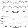 |
Fig. 1 The top panel shows the input spectra from August 10 a) and August 13 b) that correspond to the phases 0.43 and 0.64, with the input S/N values of 99.3 and 102.1, respectively. The lower panel shows the LSD profile correspondence of the related spectrum with the deconvolved S/N values 935 and 943. A part of the wavelength region is plotted in order to more clearly represent the quality of observations. |
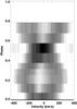 |
Fig. 2 LSD profiles obtained for the spectra on the night of August 10. |
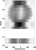 |
Fig. 3 LSD profiles obtained for the spectra on the night of August 13. |
The S/N values for the spectra of August 10 vary between 44.8 and 107.2 with an average value of 88.3. The spectra on August 13 have a S/N ranging from 55.6 to 102.1, which corresponds to an average value of 87.0. The LSD process yielded an average S/N value of 945.5 for August 10 and 998.2 for August 13.
3. System parameters
We use the latest version of the surface mapping code DoTS (Collier Cameron 1997) to image both components of this contact binary system. As described in Collier Cameron (1997), the system computes the Roche potential of the stellar system and both gravity darkening and reflection effects can be adjusted. Modifications were made to this code by Barnes et al. (2004) to allow full contact systems to be modelled. Look up tables containing the specific intensities as a function of velocity, limb angle, and effective temperature for each star are used to compute the intensity contribution of each element across the stellar surface. The parameter being mapped is the brightness (flux) distribution across the stellar surface(s). This flux distribution is calculated using a spot filling factor for each surface element, where a filling factor can vary between 0 and 1.0, implying zero and total spot coverage, respectively. The code employs maximum entropy to find a unique spot solution that fits the dataset to the required level. As demonstrated in several previous papers, (e.g. Unruh & Collier Cameron 1995; Barnes et al. 1998, 2004), this code can be used to measure system parameters (e.g., K1 and K2) and line parameters (e.g., EW) by fixing other parameters to the nominal values and measuring the values of variables by minimising the chi-squared. Extensive tests in these previous papers have shown that this method enables us to recover more precise system parameters and spot maps with fewer artifacts.
To produce accurate spot surface maps of stars, it is necessary to fine-tune the fundamental system parameters (e.g. Vgam – the center-of-mass velocity of the system). Inaccurate system parameter measurements introduce artefacts into the surface reconstructions (Unruh 1996). The determination of the system parameters can be performed by the minimization of χ2 using a fixed number of maximum entropy regularized iterations to obtain a fit to the profiles (e.g. Barnes et al. 1998). Here, we applied the same method using the LSD profiles obtained from observational data. DoTS can be used in this context, with an adjustment of a number of parameters to obtain a minimum χ2 value after several iterations. This value can also be determined with an interpolation by plotting χ2 values versus the adjusted parameter spaces. The procedure followed to find the optimal system parameters is described below, in more detail.
For binary systems, several key parameters must be measured. Figure 4 is a simplified schematic diagram showing which properties of the line profiles are most affected by varying both the stellar parameters and the LSD line strength (EW). The center-of-mass velocity Vgam is relatively independent as it affects only the global velocity of the system. Parameters such as q (mass ratio) and K1,2 (velocity amplitudes of the components) are more sensitive to the shape of the profiles while the parameters Teff1,2 (effective temperatures of the components) and EW1,2 (line intensity) mostly affect the width and the depth. Thus, we decided to determine the orbital parameters as a first assumption. We used the values (q, K1, Vgam) from Rucinski et al. (2005) as the preliminary parameter set, which is compatible with our LSD profiles. The zero-point ephemeris and the orbital period of the system (T0, P) were estimated from the 2009 BVR light curves that obtained using the 40 cm Schmidt Cassegrain Kreiken Telescope at the Ankara University Observatory (Şenavcı et al., in prep.). The related values are corrected using the recent photoelectric times of minima (spanning five years) and are in accordance with the complicated O-C behaviour of the system.
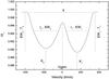 |
Fig. 4 This diagram shows how basic system parameters affect fits to the observed data. The center-of-mass velocity, Vgam, controls the radial velocity offset of the line profiles. The K1 and K2 velocities determine the maximum relative separation of the line profile contributions from both components. The radii of both components, r1 and r2, with the line EW determine the fit to the width and strength of the line profiles, while the mass ratio, q, determines the overall width depending on the K1 and K2 velocities. The surface temperatures of both components, T1 and T2, with the line EW parameter control the the strength of the line profiles. |
In the case of the overcontact solution with DoTS, the primary radius parameter (r1) is used to set the degree of the Roche lobe filling factor (f), while the secondary radius parameter (r2) is not used because of the overcontact binarity nature of such systems. Thus, during the analysis, we used the Roche lobe filling factor (f) determined from the 2001–2010 light curve analysis of SW Lac (Şenavcı et al., in prep.), which is also in accordance with the related value determined by Albayrak et al. (2004), Gazeas et al. (2005), and Alton & Terrell (2006).
SW Lac is a W-type W UMa contact binary star, which means the more massive component is closer to the observer during the primary minimum. For this reason, we used a q value bigger than one during the analysis. We performed a three-dimensional grid search for the parameters q, K1, and f. We adjusted the q parameter within the large error limits given by Rucinski et al. (2005).
We carried out two-dimensional grid searches for EW1,2 and Teff1,2 parameter sets, which allowed us to optimise fits to the LSD profile depths. A sample of these grid searches is given in Fig. 5. We determined the surface temperatures of the components from a 2009 light curve analysis of the system to be T1 = 5470 K and T2 = 5194 K (Şenavcı et al., in prep.). Thus, we used these values as the preliminary values during the two-dimensional grid search for the Teff1,2 parameter set. We obtained the surface temperatures as T1 = 5390 K and T2 = 5170 K, which is consistent with the spectral type of the system.
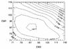 |
Fig. 5 Two-dimensional grid search for EW1,2. Here, contour numbers represent the χ2 values for the related grid. |
The Vgam value obtained during the analysis is in accordance with the value obtained by Rucinski et al. (2005). The well-known orbital inclination (i) from the photometric studies were also redetermined during the analysis. Reflection effect and gravity darkening grid searches were performed in order to complete the fine tuning procedure. Preliminary values of related parameters were taken as 0.5 (Rucinski 1969) and 0.08 (Lucy 1967), respectively, appropriate for stars with convective envelopes. Linear limb-darkening coefficients were taken from Phoenix model atmospheres corresponding to the effective temperatures of both components (Hauschildt & Baron 2005).
The finalisation of the parameter optimisation (fine tuning) with the error estimation were carried out using the downhill simplex (amoeba) algorithm (Press et al. 1992) in order to search for a multidimensional space for the global minimum. The results obtained from the minimizations described here are given in Table 2.
Best fitting parameters obtained from the chi-square minimization and amoeba search.
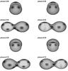 |
Fig. 6 The left panel shows the input spot model for the test. Black represents the position of dark cool spots. The right panel belongs to the reconstructed images based on the input spot model and a phase coverage similar to our combined August 10 and 13 dataset. |
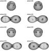 |
Fig. 7 The left panel belongs to the reconstructed images based on the partial phase coverage from August 10 2009 only, while the right panel shows the same for the phase coverage of August 13. |
4. Tests
The only previous Doppler imaging study of a contact binary system using the code DoTS, was based on a well-sampled dataset (335 spectra covering four orbital periods (Barnes et al. 2004)). Since our dataset has much poorer time-sampling, we conduct tests to evaluate the effect of our phase coverage on the reconstructed images with the contact binary option in the code. We generated ten spots with a distribution covering specific locations for each component to assess the reliability of the code in reconstructing detailed spot distributions for these systems. We performed three different tests using the spot model shown in the left panel of Fig. 6. We list the test results for the
-
complete phase coverage (Fig. 6, right panel);
-
phase coverage of August 10 data (Fig. 7, right panel);
-
phase coverage of August 13 data (Fig. 7, left panel).
The test results showed that our Doppler imaging code DoTS works well for contact binary stars except for the lower latitudes, which is a common problem for Doppler imaging (see Fig. 6 right panel). It is also clear that the code is robust enough to model the spot features located on the neck region, which is complicated because of the relatively small region it occupies when the system is projected along the line of sight.
As can be seen from Fig. 7, the code can model the spot features in spite of the missing phase coverage. However, comparing tests performed using complete phase coverage (Fig. 6 right panel) and deficient phase coverages (Fig. 7) reveals some differences. The spot filling factors obtained from the individual nights are slightly lower than those obtained from the combined nights because of the improved coverage from the combined dataset. On August 10, the filling factor is 12% lower than those obtained using the complete phase coverage, whereas the difference is 5% for August 13. On August 10, the phases covered are mainly between 0.0 and 0.5, whereas August 13 focusses on phases in the range 0.5–1.0. As a result, we are confident that the reconstructed images even with the missing phase are quite convincing, and seem almost indistinguishable from the model with complete phase coverage. On the other hand, test results show that the lack of complete phase coverage causes a considerable underestimate of the total spot coverage. This may a greater problem in the case of real observational data, where the S/N values are variable. Since the aim of these tests is to examine the robustness of the code when missing phase coverage, we performed these tests using a higher S/N value (~10 000) than those of the data. We then performed an additional test using the average of observational S/N values, to check the robustness of the reconstructions. We generated fake data with the phase coverage of our combined August 10 and 13 datasets, the same spot distribution, and a S/N value of ~972, which corresponds to the average S/N values of the August 10 and 13 datasets. The test results are given in Fig. 8.
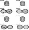 |
Fig. 8 The left panel belongs to the input spot model, while the right panel shows the images reconstructed from the fake data with an average S/N value of 972 and a phase coverage similar to our combined August 10 and 13 dataset. |
As can be seen from Fig. 8, lower S/N values such as 972, cause a considerable underestimate of the total spot coverage as mentioned above. In addition, the most notable effect in reconstructions is the extension of spot features in the latitudinal direction. This is due to the relatively low S/N of the data (i.e. the noise level relative to the starspot amplitudes in the profiles), which increases the uncertainty with which starspot latitudes can be constrained.
5. Results
As a first attempt, we obtained spot maps of the system for each night separately. We then combined the data from the two nights in order to obtain detailed high-quality surface maps of both components of SW Lac. First, images were constructed for both nights of observation. This allows us to compare the structure from each night and evaluate whether any significant spot evolution has occurred between the two epochs. If the structure is compatible, then the datasets for both nights can be combined to yield images with better phase coverage.
To obtain reliable spot maps of the system, we used the TEST statistics option of DoTS, which can be used to determine where the code begins fitting noise in the data rather than spot signatures. The TEST statistic measures the degree of non-parallelism between the gradient of the chi-square statistic and the gradient of the image entropy. When TEST tends to zero for a fixed achievable chi-square, it indicates solution convergence. However, when pushing the fit to an unachievable chi-squared value as in Fig. 9, the value of TEST begins to increase steeply, even though the chi-squared value does not continue to decrease much. This marks the point where noise begins to be fitted instead, causing the image entropy to move away from maximum. This process is performed by running the code, DoTS, using our dataset and optimal physical parameters, after setting an impossibly low chi-square value and a large number of iterations. Plotting TEST as a function of iteration number enables the determination of the aim (target) chi-squared value for our final spot maps.
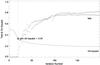 |
Fig. 9 The solid line is the chi-square variation versus iteration and the “+” symbols show the TEST statistic against iteration. The diamond symbol represents the aim chi-square value, which is chosen according to where the TEST starts to rise dramatically. |
Figure 9 represents the resultant plot after the process described above. As can be seen from the figure, at around iteration number 20, TEST values begin to steepen dramatically, marking where the noise begins to be fitted. Thus, this point is used to determine our final aim chi-square value. Application of that process using the combined datasets of SW Lac gave an aim chi-square value of 0.34 (see Fig. 9), which was used to obtain our final spot maps.
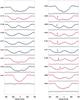 |
Fig. 10 Phase-ordered LSD profiles of August 10 (black) and 13 (red) data. Phases are shown on the left side of each profile. Solid blue lines represent the maximum entropy regularized models obtained using DoTS. The black vertical lines show residuals from the modelling of combined datasets, which also represent the uncertainties in each profile. Arrows and bars show the modelled spot features, which will be discussed in text, in detail. |
Figure 10 shows the LSD profiles and the related fits obtained using DoTS. Residuals from the modelling of combined datasets clearly shows that there are no systematic errors corresponding to the reliability of model parameters. The “hump” features that correspond to the existence of cool spots on each component are marked with arrows and bars. The features marked with arrows at the right panel between phases 0.580 and 0.835, clearly show the existence of a cool star spot on the secondary component as its migration with phase is also clearly seen. The small bars on the left panel between phases 0.067 and 0.223 show a small-scale spot feature with a low contrast on the primary component. The larger bars on the left panel between phases 0.223 and 0.432 show the modelled features that correspond to a group of small-scale spots on the secondary component. Similar features can be seen on the primary component that are indicated by bars in the right panel between phases 0.737 and 0.899.
5.1. Individual spot maps
The data obtained on August 10 cover the phases between 0.07 and 0.74. The missing phases for these images are between the secondary maximum (ph = 0.75) and the primary minimum (ph = 0.0) (see Fig. 2). The surface maps obtained using these data are shown in Fig. 11.
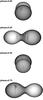 |
Fig. 11 Spot modelling using August 10 data with a phase coverage in the range 0.07–0.74. The primary component is the smaller and brighter one. |
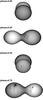 |
Fig. 12 Spot modelling using August 13 data with a phase coverage between 0.43–0.12. |
A comparison of the surface maps obtained using the data of both nights clearly shows the information loss caused by the missing phase coverage, which is discussed in detail in Sect. 6. From Fig. 11, the spot maps obtained using the August 10 dataset, it is obvious that there is no evidence of spot features during the second quadrature (ph = 0.75) on the primary component. In the case of the spot maps obtained using August 13 dataset (Fig. 12), the unspotted surface of the primary component during the first quadrature (ph = 0.25) can be clearly seen. There are also some small differences in the longitude information between the spot maps of August 10 and 13 again due to the differences in the phase coverage.
5.2. Total spot maps
The surface maps of the system obtained using the combined datasets are shown in Fig. 13. Comparison of the spot maps obtained using individual and combined datasets shows that the information loss due to the missing phase coverage, such as the amount of spot filling factors and the evidence of spot features, has been removed.
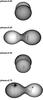 |
Fig. 13 Spot modelling using combined dataset. |
6. Discussion
The first surface mapping of the contact binary SW Lac has been carried out in this paper, using the least squares deconvolution (LSD) signal-enhancing technique and the Doppler imaging code DoTS. The maps show that both components have some spot features, which are especially dense around the phase 0.75. This is also in accordance with the B and V light curves obtained in 2009, since the light level around phase 0.75 is lower than at phase 0.25. On the other hand, the phase-dependent light modulation seen in 2001–2010 light curves is highest around phase 0.25, which may be a consequence of spot migration (Şenavcı et al., in prep.). An additional point is that the exposure times varied between 1200 and 1500 s (except one of 1065 s), which corresponds to about 4–5% of the orbital period. In this case, the phase smearing phenomenon becomes significant and prevents the resolution of the smaller spot features that can be distinguished with shorter exposures. Since we could not obtain data with a complete phase coverage for each night, it was impossible to detect the existence of spot migration from night to night.
As can be seen from Fig. 11, there is no spot feature visible on the primary component during the second quadrature (ph = 0.75). The August 10 dataset includes a spectrum with a relatively low S/N obtained during the phase 0.737, which enables us to reconstruct a big spot obviously seen on the secondary component at the same phase. The surface reconstructions of August 13 and combined datasets showed that this spot has the highest contrast and filling factor, as can be seen from Fig. 10. In addition, it is clear from Figs. 12 and 13 that the primary component has some small-scale spot distributions with a lower contrast seen at the phase 0.75 (the corresponding spot signatures are marked with bars in Fig. 10). Thus, the unspotted surface of the primary component seen in Fig. 11 can be associated primarily with the lack of phase coverage between phases 0.74 to 0.07, though the low S/N and the small, harder-to-resolve spot size on this component may be additional contributing factors. In addition, the long exposure times are disadvantageous for reconstructing such tiny features.
The unspotted surface reconstruction of the primary component at the first quadrature (ph = 0.25) is an expected consequence of the data obtained on August 13 not covering the related phase. On the other hand, the surface reconstructions obtained from August 10 and the combined datasets indicate a small-scale spot feature with a low contrast on the corresponding hemisphere of the primary component (these are also found in the spectra, as marked by small bars in Fig. 10).
The group of star spots seen on the secondary component at around first quadrature, which is visible for both the August 10 and 13 datasets, are reconstructed from the “hump” features shown in Fig. 10 for the phases 0.223–0.432.
As a result, the surface reconstructions of the system revealed that the secondary (more massive) component possesses more spots than the primary, which is a characteristic of the “W-type syndrome”. This phenomenon is explained as a consequence of the relatively deep convective envelope of the secondary component, which leads to a stronger dynamo process in the more massive component (Rucinski 1992). According to the theory of Mullan (1975), the thickness of the convective envelope of the secondary component decreases because of energy transfer from the primary to the secondary, which is reconciled by the reduced activity of the secondary component. It is also known that there are some indications, such as the existence of the Hα emission feature, that the more massive components are preferentially more active (Barden 1985; Bradstreet & Guinan 1988).
6.1. Comparison with similar systems
A comparison of the results obtained here with previous related studies are presented in this section to outline the scope of this study, as well as the importance of these investigations.
We first need to clarify the definition of the primary and the secondary component used here for W-type W UMa contact binary stars. We define the primary component as the hotter but less massive one (owing to the W-type phenomenon), which is closer to the observer during the secondary minimum. The following comparisons are made based on this assumption.
Doppler imaging of the W-type W UMa contact binary AE Phe was carried out by Barnes et al. (2004), using the Doppler imaging code DoTS. They obtained 335 time-resolved spectra covering four orbital periods with an average S/N value of 130 and an exposure time of 300 s. They found that 5% of the surface of the cooler secondary component is covered by spots, while the spot coverage is 10% for the primary component, which is not in accordance with the W-type phenomenon. However, they noted that the high density of the spots scattered over the surface of the secondary component indicates that the total spot coverage should be higher than the image reconstructions are able to resolve. They also pointed out that the temperature difference of 410 K between the primary and the secondary components should be due to an additional unresolved spottedness. For SW Lac, we found the spot coverages to be 2% and 3% for the primary and secondary components, respectively. The higher spot-filling factor on the secondary component is an expected consequence of W-type W UMa contact binaries. The temperature difference of 220 K between the primary and the secondary components is also typical of these systems. However, the spot coverage difference of 1% may not be sufficient to clearly make cause this argument. In addition to the data with incomplete phase coverage on individual days, the long exposure times and the data with low S/N did not allow us to resolve many of the smaller features seen on AE Phe. Nevertheless, the difference in the photospheric temperatures implies that the secondary component possesses a larger spot coverage. This result will be clarified by TiO analysis performed soon.
It was noted that the spot features found in the neck region of each side of both components of AE Phe are darker on the leading side of each star, which may be a consequence of surface flows. In the case of SW Lac, the neck region also exhibits spot features that appear on the secondary component at phase 0.25 and the primary component at phase 0.75. But there are no counterparts of these features (or they are unable to be resolved) on the opposite side of both components as seen in AE Phe. On the other hand, this may be a consequence of surface flows on SW Lac.
It is not possible to detect the starspot evolution in SW Lac, as achieved by AE Phe, because of the lack of data with complete phase coverage each night.
Another Doppler imaging study of a contact binary star was carried out by Hendry & Mochnacki (2000). They obtained the surface maps of the W-type W UMa contact binary star VW Cep using two years of observational data. They used wavelength regions centered on the Na D lines and a resolution of 10 500–11 700 to reconstruct the surface images of the system. They also obtained time-resolved spectra centered on the Hα line, to reveal the flare activity of VW Cep. The authors discussed the feasibility of detecting Na D lines in Doppler imaging and emphasized that the dominant contribution to opacity is scattering for these lines, thus there is very little chromospheric emission. In spite of this amount of emission, they stressed that using Na D lines is the best choice to obtain spot maps for such a long-term study.
Hendry & Mochnacki (2000) found the spot coverage of the primary and the secondary (more massive) components to be 55% and 66%, respectively. These values are significantly larger than those recovered for SW Lac and AE Phe. However, we note that their maps were recovered using a different DI code, and included both simultaneous spectroscopy and photometry as inputs; this enabled the authors quantify the contribution of some of the uniform, unresolved spots, as well as the larger active regions that traditional DI is more sensitive to. In the future, simultaneously fitting the spot-sensitive molecular bands (e.g., TiO bands) in spectroscopy data would enable us to obtain a more complete picture of the total spot coverage of cool stars to be recovered. The most notable difference of the spot distribution between VW Cep and SW Lac is the lack of features near the neck region of VW Cep. In addition, the only spot feature near the pole is near 80° latitude on the secondary component of SW Lac, though the existence of polar spots are common in AE Phe and VW Cep. However, the absence of polar spots in the reconstructed images of SW Lac have some uncertainties as it could be a consequence of smeared-out profiles due to the long exposure times (1065–1500 s) compared with those of AE Phe (300 s) and VW Cep (400 s).
6.2. Comparison with other systems
One of the most recent Doppler imaging studies of the magnetically active single star AB Dor was carried out by Jeffers et al. (2007). They reconstructed the surface maps of the star using datasets spanning from 1988 to 1994. Their results show that the star is covered by a long-lived stable polar spot and high to low latitude spots. They also mentioned that the reconstructions show preferred longitudes, while they could not find another spot concentration that is a consequence of active longitudes or flip-flop cycles. As for AB Dor, the young K0 dwarf LQ Hya nearly has the same spot characteristics, while active longitudes were found by Berdyugina et al. (2002).
In the case of SW Lac, unlike the single cool stars mentioned above, the mixture of high and low latitude spot characteristics is not apparent in the surface maps of the system. This picture seems nearly the same for AE Phe. However, both components of the contact binary VW Cep show high to low latitude spots. In addition, from the reconstructed images of SW Lac, the presence of preferred longitudes is not clear as in the case of AE Phe. On the other hand, from the long-term observations of VW Cep, Hendry & Mochnacki (2000) determined the presence of an active longitude on the secondary component of the system. Since the spectral observations of SW Lac cover a very short time-span, it is not possible to draw any conclusion about either spot migration or active longitudes. However, Oláh (2006) suggested that the common magnetic fields and the tidal forces are the main forces affecting the flux tube eruption on the stellar surfaces of close binary stars with cool components (i.e. RS CVn-type close binaries). The author also mentioned that the binaries with smaller orbits, short orbital periods, and mass ratios closer to unity have active longitudes around quadrature phases, depending on the close binary sample in her study. This is also in accordance with Demircan (1990)’s suggestion that the stellar activity may depend on the size of the orbit and the mass ratio. In the case of SW Lac, the orbital period, size of the orbit, and the value of mass ratio ensure that this is indeed the case, along with the spot concentration around the quadrature phases seen from the surface reconstruction of the system. Since the mass ratio of the system is close to unity (q = 1.280) and the components are the main-sequence stars, the dominating effect should be that of the common magnetic field rather than tidal effects. In addition, several assumptions are usually made (e.g. Mestel 1984; Guinan & Giménez 1993; Selam & Demircan 1994; Demircan 1999) that the short-period RS CVn binaries, as in the sample list of Oláh (2006), are probably the progenitors of W-type contact binaries such as SW Lac.
7. Conclusion
We have reconstructed the first surface maps of the W-type contact binary SW Lac, as part of the detailed investigation of the surface inhomogeneities of the system. In addition to deriving surface maps, we have also redetermined some physical parameters of the system using the Doppler imaging code DoTS. The length of the exposure times and the data with missing phase coverage prevented us from resolving small-scale spot distributions and investigating the short timescale activity behavior of the system. However, test results have proven the reliability of the maps and the robustness of the code in spite of the data with missing phase coverage.
The 1% increase in spottedness of the secondary component is compatible with the definition of W-type contact binaries. However, the amount of this difference is uncertain and could be higher, because of the difficulties mentioned above. To enlighten this uncertainty and obtain more information about the spot filling factors of both components, a TiO band analysis will be performed as another part of this study. Furthermore, spot features seen on both components around first quadrature (ph = 0.25) and on the primary component around second quadrature (ph = 0.75) seem to have lower contrasts and scattered structures than the spot feature seen on the secondary component around second quadrature. These ambiguities arising from the major problems described above, negatively affect the reliability of related features. Nevertheless, a comparison of 2002 and 2009 light curves of the system significantly supports the existence of cool spots, especially around the first quadrature.
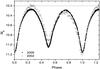 |
Fig. 14 A comparison of 2002 and 2009 B-band light curves of SW Lac. |
Figure 14 compares 2002–2009 B-band light curves of SW Lac obtained at the Ankara University Observatory using the Hamamatsu SSP5-A photomultiplier tube attached to a 30 cm Maksutov Telescope and Apogee Alta U47 CCD camera attached to a 40 cm Schmidt Cassegrain Kreiken Telescope, respectively. Standard magnitude transformation is applied to prevent any instrumental effects. Since there is no unspotted (“clean”) light curve of the system, we used the 2002 light curve for comparison, which has the highest light level recorded within the data between 2001–2010. As can be seen from Fig. 14, the effect of stellar spot(s) is clear around the first quadrature, as well as the second quadrature. In addition, the second quadrature is more affected then the first one, which is also in accordance with the surface reconstructions of SW Lac. Thus, the reconstructed spots on each component seems reliable, except for the spot filling factor parameters.
The surface reconstructions of the contact binary SW Lac are also important for increasing the samples, to more clearly understand the evolutionary status of these systems. These results will be strengthened with the help of the detailed light curve and period analysis, using the data spanning 10 years and 119 years, respectively.
Acknowledgments
The authors would like to thank J.-F. Donati for making his LSD code available for this study and T. Şahin for his assistance during the
observations at the McDonald Observatory. H. V. Şenavcı gratefully acknowledges the support of TÜBİTAK (The Scientific and Technological Research Council of Turkey) for TÜBİTAK – BİDEB – 2214 scholarship. Finally, we would like to thank the anonymous referee that helped us strengthen and improve the paper.
References
- Albayrak, B., Djurašević, G., Erkapić, S., & Tanrıverdi, T. 2004, A&A, 420, 1039 [NASA ADS] [CrossRef] [EDP Sciences] [Google Scholar]
- Alton, K. B., & Terrell, D. 2006, Journal of the American Association of Variable Star Observers (JAAVSO), 34, 188 [NASA ADS] [Google Scholar]
- Barden, S. C. 1985, ApJ, 295, 162 [NASA ADS] [CrossRef] [Google Scholar]
- Barnes, J. R., Collier Cameron, A., Unruh, Y. C., Donati, J. F., & Hussain, G. A. J. 1998, MNRAS, 299, 904 [NASA ADS] [CrossRef] [Google Scholar]
- Barnes, J. R., Lister, T. A., Hilditch, R. W., & Collier Cameron, A. 2004, MNRAS, 348, 1321 [NASA ADS] [CrossRef] [Google Scholar]
- Berdyugina, S. V., Pelt, J., & Tuominen, I. 2002, A&A, 394, 505 [NASA ADS] [CrossRef] [EDP Sciences] [Google Scholar]
- Binnendijk, L. 1960, AJ, 65, 358 [NASA ADS] [CrossRef] [Google Scholar]
- Binnendijk, L. 1970, Vistas Astron., 12, 217 [NASA ADS] [CrossRef] [Google Scholar]
- Bradstreet, D. H., & Guinan, E. F. 1988, ESA SP, 281, 303 [NASA ADS] [Google Scholar]
- Brownlee, R. R. 1957, ApJ, 125, 372 [NASA ADS] [CrossRef] [Google Scholar]
- Collier Cameron, A. 1997, MNRAS, 287, 556 [NASA ADS] [CrossRef] [Google Scholar]
- Cruddace, R. G., & Dupree, A. K. 1984, ApJ, 277, 263 [NASA ADS] [CrossRef] [Google Scholar]
- Demircan, O. 1990, in Active Close Binaries Proceedings, NATO Advanced Study Institute, ed. C. Ibanoğlu, NATO ASIC Proc., 319, 431 [Google Scholar]
- Demircan, O. 1999, Turkish J. Phys., 23, 425 [NASA ADS] [Google Scholar]
- Donati, J., Semel, M., Carter, B. D., Rees, D. E., & Collier Cameron, A. 1997, MNRAS, 291, 658 [NASA ADS] [CrossRef] [MathSciNet] [Google Scholar]
- Eaton, J. A. 1983, ApJ, 268, 800 [NASA ADS] [CrossRef] [Google Scholar]
- Gazeas, K. D., Baran, A., Niarchos, P., et al. 2005, Acta Astron., 55, 123 [NASA ADS] [Google Scholar]
- Guinan, E. F., & Giménez, A. 1993, in Astrophysics and Space Science Library, ed. J. Sahade, G. E. McCluskey Jr., & Y. Kondo, 177, 51 [Google Scholar]
- Hauschildt, P., & Baron, E. 2005, Mem. Soc. Astron. Ital. Suppl., 7, 140 [NASA ADS] [Google Scholar]
- Hendry, P. D., & Mochnacki, S. W. 1998, ApJ, 504, 978 [NASA ADS] [CrossRef] [Google Scholar]
- Hendry, P. D., & Mochnacki, S. W. 2000, ApJ, 531, 467 [NASA ADS] [CrossRef] [Google Scholar]
- Jeffers, S. V., Donati, J., & Collier Cameron, A. 2007, MNRAS, 375, 567 [NASA ADS] [CrossRef] [Google Scholar]
- Jeong, J. H., Kang, Y. W., Lee, W. B., & Sung, E. C. 1994, ApJ, 421, 779 [NASA ADS] [CrossRef] [Google Scholar]
- Kupka, F., Piskunov, N., Ryabchikova, T. A., Stempels, H. C., & Weiss, W. W. 1999, A&AS, 138, 119 [NASA ADS] [CrossRef] [EDP Sciences] [MathSciNet] [PubMed] [Google Scholar]
- Lucy, L. B. 1967, ZAp, 65, 89 [NASA ADS] [Google Scholar]
- McCarthy, J. K., Sandiford, B. A., Boyd, D., & Booth, J. 1993, PASP, 105, 881 [NASA ADS] [CrossRef] [Google Scholar]
- Mestel, L. 1984, in Cool Stars, Stellar Systems, and the Sun, ed. S. L. Baliunas, & L. Hartmann, Lecture Notes in Physics (Berlin Springer Verlag), 193, 49 [Google Scholar]
- Mullan, D. J. 1975, ApJ, 198, 563 [NASA ADS] [CrossRef] [Google Scholar]
- O’Connell, D. J. K. 1951, MNRAS, 111, 642 [NASA ADS] [Google Scholar]
- Oláh, K. 2006, Ap&SS, 304, 145 [NASA ADS] [CrossRef] [Google Scholar]
- Popper, D. M. 1980, ARA&A, 18, 115 [NASA ADS] [CrossRef] [Google Scholar]
- Press, W. H., Teukolsky, S. A., Vetterling, W. T., & Flannery, B. P. 1992, Numerical recipes in C. The art of scientific computing, ed. W. H. Press, S. A. Teukolsky, W. T. Vetterling, & B. P. Flannery [Google Scholar]
- Pribulla, T., & Rucinski, S. M. 2006, AJ, 131, 2986 [NASA ADS] [CrossRef] [Google Scholar]
- Rucinski, S. M. 1969, Acta Astron., 19, 245 [Google Scholar]
- Rucinski, S. M. 1992, in The Realm of Interacting Binary Stars, ed. J. Sahade, G. E. McCluskey, & Y. Kondo, Astrophysics and Space Science Library, 177, 111 [Google Scholar]
- Rucinski, S. M., Brunt, C. C., Pringle, J. E., & Vilhu, O. 1984, MNRAS, 208, 309 [NASA ADS] [CrossRef] [Google Scholar]
- Rucinski, S. M., Pych, W., Ogłoza, W., et al. 2005, AJ, 130, 767 [NASA ADS] [CrossRef] [Google Scholar]
- Rucinski, S. M., Pribulla, T., & van Kerkwijk, M. H. 2007, AJ, 134, 2353 [NASA ADS] [CrossRef] [Google Scholar]
- Selam, S. O., & Demircan, O. 1994, Mem. Soc. Astron. Ital., 65, 405 [NASA ADS] [Google Scholar]
- Stȩpień, K., Schmitt, J. H. M. M., & Voges, W. 2001, A&A, 370, 157 [NASA ADS] [CrossRef] [EDP Sciences] [Google Scholar]
- Straizys, V., & Kuriliene, G. 1981, Ap&SS, 80, 353 [NASA ADS] [CrossRef] [Google Scholar]
- Struve, O. 1948, PASP, 60, 160 [NASA ADS] [CrossRef] [Google Scholar]
- Unruh, Y. C. 1996, in Stellar Surface Structure, ed. K. G. Strassmeier, & J. L. Linsky, IAU Symposium, 176, 35 [Google Scholar]
- Unruh, Y. C., & Collier Cameron, A. 1995, MNRAS, 273, 1 [NASA ADS] [Google Scholar]
- Vogt, S. S. 1981, ApJ, 247, 975 [NASA ADS] [CrossRef] [Google Scholar]
All Tables
Best fitting parameters obtained from the chi-square minimization and amoeba search.
All Figures
|
Fig. 1 The top panel shows the input spectra from August 10 a) and August 13 b) that correspond to the phases 0.43 and 0.64, with the input S/N values of 99.3 and 102.1, respectively. The lower panel shows the LSD profile correspondence of the related spectrum with the deconvolved S/N values 935 and 943. A part of the wavelength region is plotted in order to more clearly represent the quality of observations. |
| In the text | |
|
Fig. 2 LSD profiles obtained for the spectra on the night of August 10. |
| In the text | |
|
Fig. 3 LSD profiles obtained for the spectra on the night of August 13. |
| In the text | |
|
Fig. 4 This diagram shows how basic system parameters affect fits to the observed data. The center-of-mass velocity, Vgam, controls the radial velocity offset of the line profiles. The K1 and K2 velocities determine the maximum relative separation of the line profile contributions from both components. The radii of both components, r1 and r2, with the line EW determine the fit to the width and strength of the line profiles, while the mass ratio, q, determines the overall width depending on the K1 and K2 velocities. The surface temperatures of both components, T1 and T2, with the line EW parameter control the the strength of the line profiles. |
| In the text | |
|
Fig. 5 Two-dimensional grid search for EW1,2. Here, contour numbers represent the χ2 values for the related grid. |
| In the text | |
|
Fig. 6 The left panel shows the input spot model for the test. Black represents the position of dark cool spots. The right panel belongs to the reconstructed images based on the input spot model and a phase coverage similar to our combined August 10 and 13 dataset. |
| In the text | |
|
Fig. 7 The left panel belongs to the reconstructed images based on the partial phase coverage from August 10 2009 only, while the right panel shows the same for the phase coverage of August 13. |
| In the text | |
|
Fig. 8 The left panel belongs to the input spot model, while the right panel shows the images reconstructed from the fake data with an average S/N value of 972 and a phase coverage similar to our combined August 10 and 13 dataset. |
| In the text | |
|
Fig. 9 The solid line is the chi-square variation versus iteration and the “+” symbols show the TEST statistic against iteration. The diamond symbol represents the aim chi-square value, which is chosen according to where the TEST starts to rise dramatically. |
| In the text | |
|
Fig. 10 Phase-ordered LSD profiles of August 10 (black) and 13 (red) data. Phases are shown on the left side of each profile. Solid blue lines represent the maximum entropy regularized models obtained using DoTS. The black vertical lines show residuals from the modelling of combined datasets, which also represent the uncertainties in each profile. Arrows and bars show the modelled spot features, which will be discussed in text, in detail. |
| In the text | |
|
Fig. 11 Spot modelling using August 10 data with a phase coverage in the range 0.07–0.74. The primary component is the smaller and brighter one. |
| In the text | |
|
Fig. 12 Spot modelling using August 13 data with a phase coverage between 0.43–0.12. |
| In the text | |
|
Fig. 13 Spot modelling using combined dataset. |
| In the text | |
|
Fig. 14 A comparison of 2002 and 2009 B-band light curves of SW Lac. |
| In the text | |
Current usage metrics show cumulative count of Article Views (full-text article views including HTML views, PDF and ePub downloads, according to the available data) and Abstracts Views on Vision4Press platform.
Data correspond to usage on the plateform after 2015. The current usage metrics is available 48-96 hours after online publication and is updated daily on week days.
Initial download of the metrics may take a while.