| Issue |
A&A
Volume 529, May 2011
|
|
|---|---|---|
| Article Number | A2 | |
| Number of page(s) | 12 | |
| Section | Extragalactic astronomy | |
| DOI | https://doi.org/10.1051/0004-6361/201015241 | |
| Published online | 18 March 2011 | |
Multi-frequency VLBA study of the blazar S5 0716+714 during the active state in 2004
II. Large-scale jet kinematics and the comparison of the different methods of VLBI data imaging as applied to kinematic studies of AGN
1
Department of Physics and AstronomyUniversity of Turku, Tuorla Observatory, Väisäläntie 20, 21500 Piikkiö, Finland
e-mail: eliras@utu.fi; takalo@utu.fi
2
Central (Pulkovo) Astronomical Observatory, Russian Academy of Sciences, 65-1, Pulkovskoe Shosse., 196140 St. Petersburg, Russia
e-mail: bajkova@gao.spb.ru
3
Pushchino Radio Astronomy Observatory, Lebedev Physical Institute, 53, Leninskii Prosp., 119991 Moscow, Russia
e-mail: yuvet@sci.lebedev.ru
4
Joint Institute for VLBI in Europe, 4, Oude Hoogeveensedijk, Dwingeloo, 7991 PD, The Netherlands
e-mail: mahmud@jive.nl
Received: 18 June 2010
Accepted: 12 January 2011
Context. We study the jet kinematics of the blazar S5 0716+714 during its active state in 2003–2004 with multi-epoch VLBI observations.
Aims. We present a kinematic analysis of the large-scale (0–12 mas) jet of 0716+714, based on the results of six epochs of VLBA monitoring at 5 GHz. Additionally, we compare kinematic results obtained with two imaging methods based on different deconvolution algorithms.
Methods. The blazar 0716+714 has a diffuse large-scale jet, which is very faint compared with the bright compact core. Experiments with simulated data showed that the conventional data reduction procedure based on the CLEAN deconvolution algorithm does not perform well in restoring this type of structure. This might be the reason why previous kinematic studies of this source yielded ambiguous results. In order to obtain accurate kinematics of this source, we independently applied two imaging techniques to the raw data: the conventional method, based on difference mapping, which uses CLEAN deconvolution, and the generalized maximum entropy method (GMEM) realized in the VLBImager package developed at the Pulkovo Observatory in Russia.
Results. The results of both methods give us a consistent kinematic scenario: the large-scale jet of 0716+714 is diffuse and stationary. Differences between the inner (0–1 mas) and outer (1–12 mas) regions of the jet in brightness and velocity of the components could be explained by the bending of the jet, which causes the angle between the jet direction and the line of sight to change from ~5° to ~11°.
Conclusions. We tested the performance of the two imaging methods on real data and found that they yield similar kinematic results, but determination of the jet component positions by the conventional method was less precise. The method based on the GMEM algorithm is suitable for kinematic studies. It is especially effective for dim diffuse sources with the average brightness of several mJy with bright point-like features. For the source 0716+714, both methods worked at the limit of their capability.
Key words: BL Lacertae objects: individual: S5 0716+714 / galaxies: jets / radio continuun: galaxies / techniques: image processing / techniques: interferometric
© ESO, 2011
1. Introduction
The blazar S5 0716+714 at redshift z = 0.31 (Nilsson et al. 2008) is one of the most active sources of its class. It is highly variable on timescales from hours to months across all observed wavelengths. Intra-day variability (IDV) has been detected in this blazar (Wagner et al. 1996; Stalin et al. 2006; Montagni et al. 2006; Gupta et al. 2009). The IDV in radio band is likely to be intrincic to the source because it is either reported to be correlated with the optical band (Wagner et al. 1996) or its spectrum is not consistent with the scintillation (Fuhrmann et al. 2008), which implies the presence of very small emitting regions within the source. At larger time scales this source has frequent flares in both radio and optical bands. Amplitudes of the flares increased abruptly after the year 2003 (e.g. Raiteri et al. 2003; Nesci et al. 2005; Bach et al. 2007; Fuhrmann et al. 2008, and references therein). In 2007 and 2008 it was also detected at very high-energy gamma rays with the MAGIC telescope (Kranich & the MAGIC collaboration 2009; Anderhub et al. 2009).
At the milliarcsecond scale (VLBI observations) 0716+714 has a core-dominated structure with a bright point-like core and a faint diffuse jet pointing at the position angle of ~20°. At the scale of arcseconds (VLA observations), the source structure is also core-dominated, its jet is double-sided, located along the position angle of ~100° (misaligned with the milliarcsecond scale jet by ~80°), and has extended diffuse lobes (Wagner et al. 1996).
The long-term kinematics of this source have been extensively studied, and two mutually exclusive models have been suggested: one implies relatively fast outward motion of the superluminal components in the jet with speeds ranging from 5c to 16c (“fast scenario”, Bach et al. 2005), and the other claims the jet to be stationary, with significant non-radial (“precession”) motion of the jet as a whole (“stationary scenario” Britzen et al. 2009). Both these scenarios are based on the reanalysis of historical VLBI observations that span the years 1992–2001 (“fast”) and 1992–2006 (“stationary”) at frequencies from 5 to 43 GHz.
Our analysis of the inner jet kinematics of 0716+714 at frequencies of 22, 43, and 86 GHz also revealed a fast-moving jet with apparent speeds from 8c to 19c on the spatial scale from 0 to 1.5 mas (Rastorgueva et al. 2009). Here we present results of our short-term kinematic study at 5 GHz. The data set covers six months, and the source was observed nearly every month. With this dense data sampling we are able to study the fast structural changes in the jet of 0716+714.
The standard method of VLBI data reduction, which is used by the vast majority of researchers in the field, includes the Difmap package (Shepherd 1997) as an imaging facility, which became conventional because of its simplicity and accessibility. However, Difmap has its downsides, and the main disadvantage of this package, which uses the standard CLEAN algorithm by Högbom (1974; Shepherd et al. 1994), is a problem with the reconstruction of extended emission (Cornwell 1983). Tests performed on the simulated data have shown that the standard CLEAN, and Difmap in general, are especially inaccurate in the reconstruction of the sources whose structure could be described as bright point-like knots embedded in a region with faint extended emission (e.g. Baikova 2007; Lawson et al. 2004). The morphology of 0716+714 at lower frequencies (5–1.6 GHz) is consistent with this description. Therefore, a conventional approach to this source may have yielded erroneous results. In order to make sure that the structure of 0716+714 is correctly reconstructed, we independently applied both the generalized maximum entropy method (GMEM) and the conventional CLEAN to the same data set.
This paper is arranged as follows: Sect. 2 describes the observations, Sect. 3 contains a description of the a-priori data calibration and an introduction to the imaging methods. In Sect. 4 we present and discuss the kinematic results. The final kinematic scenario, a comparison with previous studies, and possible explanations of the apparent speed differences are presented in Sect. 5.
2. Observations
We observed 0716+714 with the Very Long Baseline Array (VLBA) five times during the year 2004. Each observing session lasted nine hours and covered five frequencies (86, 43, 22, 5 and 1.6 GHz) in dual polarization mode. Here we describe the results of the 5 GHz observations. The five epochs in our experiment were named in alphabetical order: A, Feb. 10; B, May 03; C, Jun. 18; D, Jul. 29 and E, Aug. 29, 2004. Additionally, we used one epoch from the unpublished polarization observation project of 37 northern BL Lac objects from the Kuehr & Schmidt sample (Kuehr & Schmidt 1990) by Gabuzda and Mahmud, in our notation epoch M, Mar. 22, 2004. Epoch M fills the gap between A and B of our experiment, making the time sampling almost uniform with an interval of approximately one month between observations.
3. Data reduction
3.1. Calibration
The data were correlated at the Socorro VLBA correlator. A-priori amplitude and phase calibration were made at Tuorla Observatory with NRAO’s Astronomical Image Processing System (AIPS). AIPS’s standard VLBAPROC procedures were used for the amplitude and phase calibrations, scans on 3C 279 were used to calculate instrumental delay and phase residuals, and OJ287 was used as an instrumental polarization (D-term) calibrator. The subsequent procedure for our two methods is described below.
3.2. Image reconstruction: the conventional method
The first method we used was the conventional method, which is a combination of CLEAN deconvolution (Högbom 1974) with self-calibration and uv-plane Gaussian model fitting. This method is used by most of the astronomical community in studies of outflow structure and kinematics.
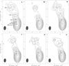 |
Fig. 1 Images of 0716+714 obtained using the conventional method: CLEAN maps, convolved with the averaged beam of 1.5 × 2.5 mas, PA = −4.5°. Circles with crosses are the Modelfit Gaussian components superimposed on the image. The Gaussian model fitting was performed in the uv-plane. Axes are right ascension and declination in milliarcseconds, measured with regard to the core. |
We used the Caltech Difmap package (Shepherd 1997) for imaging, employing a CLEAN algorithm in a self-calibration loop: a model of the source, consisting of point-like clean-components is created with CLEAN, then the antenna gains are self-calibrated with the model, and the procedure is repeated. Self-calibrations were performed in the following way: several phase self-calibration loops were followed by an amplitude one, with the solution interval of amplitude self-calibration gradually decreasing from the time of the whole observation to the data averaging time (0.5 min). Finally, we performed amplitude self-calibration with the solution interval equal to the averaging time. Then the final clean-component model was discarded, and a new source model was created. We used the Difmap procedure, Modelfit, to create a model consisting of circular components with a Gaussian distribution of flux, and fit it to the visibility data. Except for one case, only circular Gaussian components were used to parameterize the data in order to reduce the number of free parameters. For all models, the brightest optically thick component at the southernmost end of the jet was considered to be the core, as in the previous research. Positions of other components were measured with regard to this. The resulting maps with the superimposed model components are presented in Fig. 1, and map parameters for all epochs are listed in Table 1.
Map parameters for the conventional method.
The errors of the position and the flux estimates of the components were calculated with the Difwrap package (Lovell 2000), where the parameter to be analyzed (position, flux or FWHM) is varied around the best-fit value in a grid of a given step size and Modelfit is run for each step. The result of this process is plotted as a χ2 distribution, and the user can visually inspect the model vs. a uv-data plot or a residual map for each point of the grid. Visual inspection is based on the relative χ2 changes. Because the number of degrees of freedom of the model are not exactly known, this method of error estimate based on visual inspection yields more reliable results than the standard χ2 analysis. In our case it was not possible to use the model vs. a visibility plot, because we dealt with very faint components of the jet: changes in the model visibilities between different grid points were too small to be detected with the naked eye. Instead, we estimated the goodness of fit based on the appearance of the residual map and its changes from one grid point to another. We applied an intuitive criterion proposed by Savolainen (2006) to determine the maximal acceptable deviation from the best-fit model: the difference between a model and observed data is considered significant if the structure appearing in the residual map would look strong enough that it should be cleaned, if it had appeared during the imaging process. Because the flux of such a feature changes gradually from one grid point to another, it may be difficult to determine at which step the discrepancy between the observed data and the model becomes large enough. In these cases we used an empirical “2σ-rule”, which we worked out by analysis of both the imaging process and the error estimate procedure: the flux is considered ‘excessive’ and should be “cleaned out” by placing a model component in its location if the rms noise in the area under scrutiny is twice as high as the average rms noise at the outskirts of the map. At the grid point where the noise level exceeds twice the rms, we assumed that the parameter value had reached the limit. This deviation from the best-fit value was assumed to be the limiting error, Δ. A more detailed discussion of VLBI data error estimate with Difwrap and a comparison with the method of variance about the best fit can be found in Savolainen (2006).
In most cases the Difwrap package yields asymmetric uncertainties for the model parameters, which leads to a bias in the resulting models. This bias was corrected for with the method suggested by D’Agostini (2003), based on the probabilistic approach to the bias correction: let us assume that the negative limiting error of the component’s separation from the core r is Δnegr, and the positive limiting error is Δpos, and Δneg ≠ Δpos. We calculated the unbiased limiting error as an arithmetic average of the two limiting errors: Δun = (Δneg + Δpos)/2. The standard deviation of r was calculated as σr = Δun/3. The unbiased value of the model parameter (in this case, separation from the core) is not equal to the result of the model fitting and is run = r + (Δpos − Δneg)/2.
3.3. Image reconstruction: the maximum entropy method (MEM), an attempt
Another popular deconvolution algorithm in radio interferometry is the maximum entropy method invented by Jaynes (Jaynes 1957), which was first applied to image reconstruction by Frieden (Frieden 1972). The maximum entropy method is an extremely nonlinear method that leads to maximally smoothed images subject to constraints. The positivity of the sought-for solution forces super-resolution on bright isolated objects.
There are many forms of entropy (Narayan & Nityananda 1986). We used the AIPS task VTESS, which uses the entropy functional in the form (Cornwell 1995) ![\begin{eqnarray} \label{cornwell_entropy} E(I)&=& -\int I(x,y)\ln[I(x,y)/M(x,y)] {\rm d}x {\rm d}y, \\[1.4mm] && I(x,y)>0, \nonumber \end{eqnarray}](/articles/aa/full_html/2011/05/aa15241-10/aa15241-10-eq25.png) (1)where M(x,y) is a default image that represents the optimum solution in the absence of data. Usually, the default image is taken to be flat or a lower resolution image.
(1)where M(x,y) is a default image that represents the optimum solution in the absence of data. Usually, the default image is taken to be flat or a lower resolution image.
Given a form of entropy, the MEM defines the best image that maximizes E(I) subject to the data constraints: 1) fit the observed visibilities Vk to within the error term ϵk: F(I) = Vk + ϵk; 2) fit the total flux: ∫I(x,y)dxdy = F0; 3) the rms error must be plausible:  .
.
In AIPS, the Cornwell-Evans algorithm (Cornwell & Evans 1985) is used for the realization of the MEM. This algorithm uses a simple Newton-Raphson approach to optimize the functional (1) subject to the constraints upon the rms and total power enforced by the Lagrange multipliers.
We made an attempt to use the MEM method to recover the faint emission of the 0716+714 jet. We imported visibility data, self-calibrated in Difmap (see Sect. 3.2), to AIPS and used the task VTESS to create the final image.
We used the task IMAGR to clean the central part of the image containing the bright core in order to avoid circular-shaped artifacts around the point-like source. Nevertheless, the image quality of this method was poor and did not allow us to correctly perform the kinematic analysis. Therefore, we conclude that the MEM method is not suitable for recovering the emission of the sources with bright point-like features and faint underlying diffuse emission.
3.4. Image reconstruction: the generalized maximum entropy method (GMEM)
The generalized maximum entropy method has been developed and implemented in the Pulkovo VLBI data reduction software package VLBImager by Baikova (2007). The mapping technique realized in this package utilizes a self-calibration algorithm (Cornwell & Fomalont 1999) combined with the GMEM (Frieden & Bajkova 1994; Baikova 2007), which is used as a deconvolution procedure.
The GMEM is designed for the reconstruction of sign-variable functions, therefore it allows one to obtain unbiased solutions. The bias of the solution is one of the problems of the conventional MEM (Cornwell et al. 1999), which may lead to a substantial nonlinear distortion of the final image if the data contain errors (Baykova 1995).
For the GMEM, the Shannon-entropy functional has the form 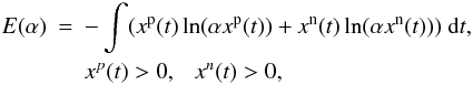 (2)where xp(t) and xn(t) are the positive and negative components of the sought-for image x(t), i.e. the equation x(t) = xp(t) − xn(t) holds. α > 0 is a parameter responsible for the accuracy of the separation of the negative and positive components of the solution x(t), and therefore critical for the resulting image fidelity. It is easy to show (Baikova 2007) that solutions for xp(t) and xn(t) obtained with the Lagrange optimization method are connected by the expression xp(t)·xn(t) = exp(− 2 − 2lnα) = K(α), which depends only on the parameter α. This parameter is responsible for dividing the positive and negative parts of the solution: the larger α is, the more accurate is the discrimination. On the other hand, the value of α is constrained by computational limitations. The main constraint comes from the χ2 term in the optimized functional, which depends on the data errors. The larger a standard deviation is, the higher value of α could be set. If data are very accurate, a lower value of α is needed. In practice, α is chosen empirically. In our case we had to compromise between data errors, which determine resolution of the resulting MEM solution, and a need to divide the positive and negative parts of the solution as accurately as possible. It is fair to say that given fixed errors in the data, a maximum possible chosen value of α provides us with the best possible resolution of the MEM-solution. In this work we used α = 100 000. The algorithm takes into account errors of the measurements. It implies a solution of the following two-dimensional problem of conditional optimization, given in the discrete form
 ![\begin{eqnarray} \label{anisa_functional} \lefteqn{\min~~\Bigg\{\sum_{k=1}^N\sum_{l=1}^N [x_{kl}^{\rm p}\ln(\alpha x_{kl}^{\rm p})+ x_{kl}^{\rm n}\ln(\alpha x_{kl}^{\rm n})]} \\\nonumber &&\qquad\qquad\qquad+\sum_{m=1}^M\frac{(\eta_m^{\rm re})^2+(\eta_m^{\rm im})^2}{\sigma_m^2}\Bigg\}, \end{eqnarray}](/articles/aa/full_html/2011/05/aa15241-10/aa15241-10-eq42.png) (3)
(3)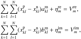 where k and l are the pixel numbers in a source map of the size N × N, m = 1,...,M is a number of the visibility function measurement,
  and
and  are the constant coefficients corresponding to the Fourier-transform,
  and
and  are the real and imaginary parts of the complex visibility function (the Fourier spectrum of a source) and
  and
and  are the real and imaginary parts of the additive visibility noise with normal distribution over zero value with known dispersion σm.
As we can see from Eq. (3), the optimized functional has two parts: a Shannon-entropy functional and a functional that is an estimate of the difference between the reconstructed visibility spectrum and the measured data according to a χ2 criterion. This latter functional can be considered to be an additional stabilizing term acting to provide a further regularization of the solution above what is possible with the entropy functional alone. Solution normalization, necessary for the MEM is obtained by limiting the total flux of the source: 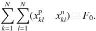 Numerical experiments show that the GMEM combined with the difference mapping technique allows the restoration of the source structures consisting of bright compact features embedded in a weaker extended background with maximal accuracy (Baikova 2007).
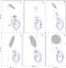 |
Fig. 2 GMEM solutions for each epoch, convolved with the averaged CLEAN beam: 1.5 × 2.5 mas, PA = −4.5°. Gray ellipses are the Gaussian components superimposed on the image. The Gaussian model-fitting was performed in the image plane for the original GMEM solutions (Fig. A.1) convolved with the beam of 0.5 × 0.5 mas (Fig. A.2). Axes are right ascension vs. declination in milliarcseconds, measured with regard to the core. |
After the a priori calibration, the raw visibility data were averaged in frequency (averaged IFs) in AIPS, then exported to Difmap, where they were rebinned, phase self-calibrated with a point source model with a 0.5 min solution interval, and finally averaged in time (over a period of four minutes). After that the data was exported to VLBImager, where the automatic GMEM deconvolution – self-calibration loop iterations were performed until convergence. The size for the maps is chosen 256 × 256 pixels with a pixel size of 0.15 mas. The GMEM solution convolved with a clean beam of ~ 2.4 × 1.5 mas, PA = −4.5° is presented in Fig. 2, and parameters for those maps are listed in Table 2.
Map parameters for the GMEM.
In the Appendix we present two additional sets of maps to demonstrate the capabilities of this deconvolution method: the original GMEM solutions (Fig. A.1) and the GMEM solutions convolved with a circular clean beam of the size 0.5 × 0.5 mas, which were used for the modeling of the source structure (Fig. A.2). The model-fitting of the maps was made in the image plane. The source structure was modeled using Gaussian elliptical components. Each of the components was described by the following six parameters: r, distance from the core (the core was determined like in the conventional method and was assumed to be stationary); φ, position angle measured counter-clockwise between the ordinate axis and the radius-vector; amaj and amin, sizes of the major and minor axes of a Gaussian ellipsoid at half maximum amplitude and θ, the angle describing the orientation of the component ellipse, an angle between the ordinate axis and the major axis of the ellipse, measured counter-clockwise. Cross-identification of the components was based on the assumption that the core separation, the position angle and the flux of the component change smoothly from epoch to epoch. In order to obtain a model of the inner jet (r < 1.5 mas) with higher accuracy, we interpolated the brightness distribution to a finer grid: the pixel size in thit case was 0.0375 mas, which was four times smaller than that for the large-scale jet. The errors of the component core separation determination were estimated by the formula (Fomalont 1999)  where σ is the rms after the subtraction of the model from the source map, Speak is the peak flux of the component, Θ is the size of the component at the amplitude half maximum (in our case we assume Θ = amaj). We point out that that this formula likely underestimates position errors, which is clear from the comparison with the Difwrap errors (see Fig. 3).
4. Results
Our aim was to study the structure and kinematics of the large-scale (from 1 to 12 mas) jet, and compare it with the results for the inner (< 1 mas) jet, which were published in Rastorgueva et al. (2009).
We applied a conventional method and a GMEM to the same data set to compare their kinematic results. For each of them, we calculated the core separation of the components as a function of time, the proper motion μ, and the apparent speeds βapp according to the formula  where the luminosity distance dL is calculated with the analytical formula derived by Pen (1999) for a flat cosmology. The same analytical expression was used by Bach et al. (2005) for their kinematic analysis of this source, therefore our results could be compared directly without conversion. For this cosmological model, a proper motion of 1 mas/yr is equivalent to the apparent speed of 19.26c. The flat Universe model with the Hubble constant of H0 = 71 km s-1 Mpc-1 and with Ωm = 0.3 and ΩΛ = 0.7 was used. We are aware that Wickramasinghe & Ukwatta (2010) recently obtained a new and more precise analytical expression for the luminosity distance, but for z = 0.3 the difference with Pen (1999) is negligible (1 mas/yr corresponds to the apparent speed of 19.22c).
The results of the Gaussian model-fitting and component identification are presented in Table 5 (conventional method) and in Table 6 (GMEM). The original GMEM-solutions are shown in Fig. A.1.
4.1. Component cross-identification between different methods.
4.1.1. Positions and apparent speeds of components
Based on core separation and fluxes, we identified four nearly stationary components in the large-scale jet of 0716+714: one at a separation of about ~1.5 mas (C3–A3), one at ~3.0 mas (C4–A4), one at ~4.6 mas (C5–A5) and one at ~12 mas (C6–A6). Their proper motions and apparent speeds can be found in Tables 3 and 4. A comparison of their positions, obtained with different methods, and linear fits are shown in Fig. 3. The components C1–C6, found by the conventional method, have a larger scatter around the mean position and larger positional errors than those of the GMEM components (compare Tables 3 and 4), which complicated the component cross-identification and made a choice of the kinematic scenario ambiguous. However, the GMEM method confirmed the stationary scenario.
However, the component C1–2, determined by the conventional method, and the component A1 found by the GMEM in the inner jet have a clear outward motion: ~10c and ~2c, respectively (Tables 3 and 4). The difference in apparent speed could be explained by the fact that the GMEM determined an extra stationary component at the separation of about 1 mas from the core (A2), while the conventional method did not. On the other hand, A2 is only found at the last four epochs, and is separated from the component A1 by only ~0.5 mas, and the component C1–2, determined by the conventional method, is located between them (see Fig. 3). Therefore, we believe that the component C1–2 is resolved by GMEM in the four last epochs, making up two components A1 and A2, and this effect causes the difference in the apparent speed.
Note that the kinematics of the outer jet are consistent with the results of Britzen et al. (2009).
Kinematic scenario obtained with the conventional method.
Kinematic scenario obtained with the GMEM.
4.1.2. Core flux
In this section we compare the ability of the two methods to restore the flux of the source. In the optically thin jet, the fluxes of the components found by the conventional method and by the GMEM agree within two sigma. At the same time, the performance of the two methods in the core region is significantly different: the conventional method places one very bright component C1–2 (the flux density is about 0.1 Jy, so it is bright compared to other jet components) next to the core, while the GMEM method finds two components, A1 and A2, with the flux density comparable to the other components in the jet (on the order of 0.01 Jy). However, if one adds up the flux densities of the core and nearby components (C0 + C1–2 and A0 + A1 + A2), the results of the two methods would agree within two sigma for all six epochs. We attribute this difference to the fact that the GMEM restores the bright point-like core accurately, whereas the conventional method, because of significantly lower resolution at 5 GHz, is likely to mix up emission of the core and of the nearby components.
5. Discussion
5.1. Inner jet kinematics: comparison of the 22 and 5 GHz data
The inner jet of 0716+714 is well resolved at higher (> 5 GHz) frequencies and reveals a clear outward motion, although the emission fades away at about 1 mas as the spectral peak moves to lower frequencies (see Rastorgueva et al. 2009). At 5 GHz, only one or two components are resolved in the inner jet region, depending on the method, and they also have a clear outward motion. Because the data at higher frequencies were reduced by the conventional method, we discussin in this section only the component C1–2. Its apparent speed can be found in Table 3. In Fig. 4 we show the motion of the component C1–2 at 5 GHz together with components C5 and C6 at 22 GHz. They are obviously located in the same area in the inner jet and have speeds of a similar values: the apparent speeds of the components C5 (22 GHz) and C6 (22 GHz) are 21.3 ± 2.5 c and 18.9 ± 0.8 c respectively, which agrees with the speed of C1–2 (5 GHz) within 3σ. The difference in the apparent speeds of the inner jet components, detected at different frequencies, is likely caused by a resolution effect.
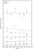 |
Fig. 3 All components obtained with the conventional and GMEM methods are shown at the same plot. |
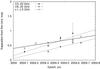 |
Fig. 4 22 GHz inner jet components C5 and C6 from Rastorgueva et al. (2009) and the component C1–2 at 5 GHz coincide spatially and have similar motion. |
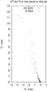 |
Fig. 5 Components of the inner and outer jet on the sky plane. The change of the orientation occurs at the distance of about 1 mas from the core. The components of the jet are well aligned, which is an indication of the collimated jet. |
5.2. Jet bending and beaming
The jet components that were found beyond 1 mas from the core at both 5 and 22 GHz have a very high dispersion in the apparent speeds, and in most cases move slower than the inner ones (see Table 3). Therefore, we observe two kinematically different regions in the jet of 0716+714: a fast moving inner jet (< 1 mas) and a slowly moving outer jet with nearly stationary components (> 1 mas). The orientation of the inner and outer parts of the jet on the sky plane are also different: the jet changes its position angle from ~ 25° (inner region) to ~ 15° (outer region). The bend occurs at the distance of about 1 mas from the core, see Fig. 5. In addition to that, we found that the flux of the jet components in the inner jet is systematically higher than the flux of the outer jet components. Based on this we propose that those effects could be caused by the jet bending away from the line of sight at the apparent distance of 1 mas from the core. We tried to find out whether it is possible to explain the observed effects by the jet bending, without additional assumptions of jet parameters. If the jet bends away from the line of sight, the beaming factor δ decreases, which causes a decrease in the apparent luminosity of the jet, because it is proportional to δ2 + α for a smooth jet (Cohen et al. 2007), where α is a spectral index (S ~ να). The apparent speed of the jet also changes with the change of the angle to the line of sight, for 0716+714 it decreases. We estimated how much the flux of the jet components change from the inner jet to the outer, and compared these results with the theoretical predictions for jet bending. We assumed the jet to be a smooth collimated flow with a constant plasma speed (and therefore constant Lorentz factor Γ). This assumption is indirectly supported by the fact that the jet components are well aligned (see Fig. 5), and the structure of the jet on VLBI maps is smooth and continuous. We used the results of the conventional method for this analysis.
For each epoch we calculated the ratio of the average component flux at 5 GHz in the outer part of the jet to the average flux at 22 GHz of the inner ones: rI = ⟨ Io ⟩ / ⟨ Ii ⟩ . Before calculating the flux ratio rI for each epoch, we corrected the spectral slope of the 5 GHz fluxes in order to compare them directly with the 22 GHz data. The 5–22 GHz spectral index α was estimated for the inner jet components C1–2 (5 GHz) and C5 and C6 (22 GHz) for each epoch separately. Individual values of the flux ratios were averaged, which gave ⟨ rI ⟩ = 0.11 ± 0.08. Assuming that the flux change is caused by jet bending, we can calculate the ratio of the beaming factors of the jet after and before the bent using the flux ratio we have just obtained: 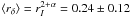 . These values were also calculated separately for each epoch, using the individual values of the spectral index, and then averaged. Errors of the averaged value consist of the standard deviation of averaging the ratios between epochs and the standard deviation of averaging the component fluxes for each epoch, added in quadrature.
The apparent kinematics of the relativistic blazar jet are determined by four parameters: the apparent speed βapp, the Lorentz factor Γ, the beaming factor δ and the angle of the jet to the line of sight Θ, any two of which could be used to find two others (e.g. Cohen et al. 2007). In the inner and outer parts of the jet, the Lorentz factor Γ is the same, but the other three parameters differ: Θ2 > Θ1, and therefore βapp2 < βapp1 and δ2 < δ1. From the 22 and 43 GHz data analysis (Rastorgueva et al. 2009) we estimated the kinematic parameters for the inner jet: the maximum apparent speed is βappmax = 19.4 and the corresponding minimum Lorentz factor is Γmin = 19.5. The corresponding minimum angle of the jet to the line of sight is Θmins = 3.0°. In the outer jet, the maximum apparent speed was βapp ≃ 10. Taking into account the above mentioned observed quantities and assuming that the jet has a constant speed, we can calculate its angle to the line of sight before (Θ1) and after (Θ2) the bending as well as other kinematic parameters of the jet.
We can consider the beaming factor of the jet as a function of the initial (inner jet) angle to the line of sight Θ1, which is larger than the Θmin = 3.0°, but smaller than the maximal value of  (all possible values lie in the lower part of a βapp − δ diagram). The ratio of the beaming factors rδ is a monotonic function of Θ1 and changes from 0.15 to 0.26, while Θ1 changes within its limits, and reaches the value of 0.24 at Θ1 = 5.2°. Therefore, the observed change of kinematics is possible if the Lorentz factor of the jet is Γ ≃ 30.0, and at the apparent distance of 1 mas from the core the jet changes its direction, with the angle to to the line of sight increasing from ~ 5° to ~ 11°. At the same time the beaming factor is changing from ~ 7 to ~ 2, respectively.
The errors of the observed flux factor ratio determination, which give us a beaming factor ratio, are fairly large, and precise calculations of the angle to the line of sight and beaming factor are not possible. The values we obtained are only estimates, and we can only say that the observed change of the jet apparent speed and brightness is possibly caused by jet bending. Also, the proposed beaming factor for the inner jet is consistent with the value found by Hovatta et al. (2009) from the radio-frequency variability.
6. Conclusions
Results from the CLEAN deconvolution-based imaging and Gaussian model fitting and component parameters.
Results from the GMEM method imaging and model fitting with component parameters.
We studied the large-scale jet kinematics of the blazar S5 0716+714 by analyzing six epochs of VLBA observations at 5 GHz. Two imaging methods were applied to this data set: a conventional method (CLEAN self-calibration loop in Difmap combined with Modelfit) and GMEM (Pulkovo VLBImager package combined with the image plane model-fitting).
6.1. Performance of the methods
S5 0716+714 has a bright point-like core and a faint diffuse jet. The emission fades down very quickly in the vicinity of the core, and the CLEAN algorithm, producing the model that is composed of the discrete point sources, is not adequately restoring this emission region. In the Gaussian model, some fraction of the core emission was added to the inner jet component, and the kinematic results were also ambiguous because of the large uncertainties of the positions of jet components.
The GMEM method delivered a smooth image of the source, which restored both the bright core and the diffuse jet. However, the jet of 0716+714 is very faint, therefore a convolution of the original solutions with the small (0.5 × 0.5 mas) beam was needed in order to obtain accurate Gaussian models of the jet structure. The original GMEM solutions convolved with the CLEAN beam in general resemble the CLEAN images (Figs. 2 and 1).
We recommend GMEM in combination with the difference mapping technique for restoring the structure of compact AGN and other objects that have a diffuse structure with bright point-like features. In addition, the original GMEM solutions have a higher resolution than other methods, and in principle they could be used directly to derive kinematics of the source, provided that the jet features are bright enough (e.g., Bajkova & Pushkarev 2008).
6.2. Structure and kinematics of the jet
The large-scale jet of 0716+714 is faint, diffuse and smooth, without prominent brightness enhancements.
Both the conventional method and GMEM deliver similar kinematic results: the large-scale jet (1–12 mas) is mostly stationary, with a large scatter of the component positions.
The position angle of the jet on the sky plane changes by ~ 10° at about 1 mas from the core.
Large-scale jet components are systematically slower and fainter than those of the inner (< 1 mas) jet components.
We attribute these last effects to the bending of the jet at the apparent distance ~ 1 mas from the core from ~ 5° to ~ 11°.
Acknowledgments
We thank the anonymous referee for the useful comments which have helped us to revise and improve the paper.
The National Radio Astronomy Observatory is a facility of the National Science Foundation operated under cooperative agreement by Associated Universities, Inc.
This study was supported in part by the “Origin and Evolution of Stars and Galaxies” – “Program of the Presidium of the Russian Academy of Sciences and the Program for State Support of Leading Scientific Schools of Russia” (NSh–3645.2010.2).
References
- Anderhub, H., Antonelli, L. A., Antoranz, P., et al. 2009, ApJ, 704, L129 [NASA ADS] [CrossRef] [Google Scholar]
- Bach, U., Krichbaum, T. P., Ros, E., et al. 2005, A&A, 433, 815 [NASA ADS] [CrossRef] [EDP Sciences] [Google Scholar]
- Bach, U., Raiteri, C. M., Villata, M., et al. 2007, A&A, 464, 175 [NASA ADS] [CrossRef] [EDP Sciences] [Google Scholar]
- Baikova, A. T. 2007, Astron. Rep., 51, 891 [NASA ADS] [CrossRef] [Google Scholar]
- Bajkova, A. T., & Pushkarev, A. B. 2008, Astron. Rep., 52, 12 [NASA ADS] [CrossRef] [Google Scholar]
- Baykova, A. T. 1995, Radiophys. Quant. Electron., 38, 828 [NASA ADS] [CrossRef] [Google Scholar]
- Britzen, S., Kam, V. A., Witzel, A., et al. 2009, A&A, 508, 1205 [NASA ADS] [CrossRef] [EDP Sciences] [Google Scholar]
- Cohen, M. H., Lister, M. L., Homan, D. C., et al. 2007, ApJ, 658, 232 [NASA ADS] [CrossRef] [Google Scholar]
- Cornwell, T. 1995, in Very Long Baseline Interferometry and the VLBA, ed. J. A. Zensus, P. J. Diamond, & P. J. Napier, ASP Conf. Ser., 82, 39 [Google Scholar]
- Cornwell, T., & Fomalont, E. B. 1999, in Synthesis Imaging in Radio Astronomy II, ed. G. B. Taylor, C. L. Carilli, & R. A. Perley, ASP Conf. Ser., 180, 187 [Google Scholar]
- Cornwell, T., Braun, R., & Briggs, D. S. 1999, in Synthesis Imaging in Radio Astronomy II, ed. G. B. Taylor, C. L. Carilli, & R. A. Perley, ASP Conf. Ser., 180, 151 [Google Scholar]
- Cornwell, T. J. 1983, A&A, 121, 281 [NASA ADS] [Google Scholar]
- Cornwell, T. J., & Evans, K. F. 1985, A&A, 143, 77 [NASA ADS] [Google Scholar]
- D’Agostini, G. 2003, Bayesian Reasoning in Data Analysis, A Critical Introduction (World Scientific), 279 [Google Scholar]
- Fomalont, E. B. 1999, in Synthesis Imaging in Radio Astronomy II, ed. G. B. Taylor, C. L. Carilli, & R. A. Perley, ASP Conf. Ser., 180, 301 [Google Scholar]
- Frieden, B. R. 1972, J. Opt. Soc. Am., 62, 511 [Google Scholar]
- Frieden, B. R., & Bajkova, A. T. 1994, Appl. Opt., 33, 219 [NASA ADS] [CrossRef] [PubMed] [Google Scholar]
- Fuhrmann, L., Krichbaum, T. P., Witzel, A., et al. 2008, A&A, 490, 1019 [NASA ADS] [CrossRef] [EDP Sciences] [Google Scholar]
- Gupta, A. C., Srivastava, A. K., & Wiita, P. J. 2009, ApJ, 690, 216 [NASA ADS] [CrossRef] [Google Scholar]
- Högbom, J. A. 1974, A&AS, 15, 417 [Google Scholar]
- Hovatta, T., Valtaoja, E., Tornikoski, M., & Lähteenmäki, A. 2009, A&A, 494, 527 [NASA ADS] [CrossRef] [EDP Sciences] [Google Scholar]
- Jaynes, E. T. 1957, Phys. Rev., 106, 620 [Google Scholar]
- Kranich, D., & the MAGIC collaboration 2009, [arXiv:0912.3830] [Google Scholar]
- Kuehr, H., & Schmidt, G. D. 1990, AJ, 99, 1 [NASA ADS] [CrossRef] [Google Scholar]
- Lawson, P. R., Cotton, W. D., Hummel, C. A., et al. 2004, in SPIE Conf. Ser. 5491, ed. W. A. Traub, 886 [Google Scholar]
- Lovell, J. 2000, in Astrophysical Phenomena Revealed by Space VLBI, Proceedings of the VSOP Symposium, ed. H. Hirabayashi, P. G. Edwards, & D. W. Murphy, 301 [Google Scholar]
- Montagni, F., Maselli, A., Massaro, E., et al. 2006, A&A, 451, 435 [NASA ADS] [CrossRef] [EDP Sciences] [Google Scholar]
- Narayan, R., & Nityananda, R. 1986, ARA&A, 24, 127 [NASA ADS] [CrossRef] [Google Scholar]
- Nesci, R., Massaro, E., Rossi, C., et al. 2005, AJ, 130, 1466 [NASA ADS] [CrossRef] [Google Scholar]
- Nilsson, K., Pursimo, T., Sillanpää, A., Takalo, L. O., & Lindfors, E. 2008, A&A, 487, L29 [NASA ADS] [CrossRef] [EDP Sciences] [Google Scholar]
- Pen, U.-L. 1999, ApJS, 120, 49 [NASA ADS] [CrossRef] [Google Scholar]
- Raiteri, C. M., Villata, M., Tosti, G., et al. 2003, A&A, 402, 151 [NASA ADS] [CrossRef] [EDP Sciences] [Google Scholar]
- Rastorgueva, E. A., Wiik, K., Savolainen, T., et al. 2009, A&A, 494, L5 [NASA ADS] [CrossRef] [EDP Sciences] [Google Scholar]
- Savolainen, T. 2006, Ph.D. Thesis, Turun Yliopisto, Turku, Finland [Google Scholar]
- Shepherd, M. C. 1997, in Astronomical Data Analysis Software and Systems VI, ed. G. Hunt, & H. Payne, ASP Conf. Ser., 125, 77 [Google Scholar]
- Shepherd, M. C., Pearson, T. J., & Taylor, G. B. 1994, in BAAS, 26, 987 [Google Scholar]
- Stalin, C. S., Gopal-Krishna, Sagar, R., et al. 2006, MNRAS, 366, 1337 [NASA ADS] [Google Scholar]
- Wagner, S. J., Witzel, A., Heidt, J., et al. 1996, AJ, 111, 2187 [NASA ADS] [CrossRef] [Google Scholar]
- Wickramasinghe, T., & Ukwatta, T. N. 2010, MNRAS, 406, 548 [NASA ADS] [CrossRef] [Google Scholar]
Appendix Appendix
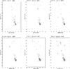 |
Fig. A.1 Original GMEM solutions. |
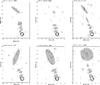 |
Fig. A.2 GMEM solutions, convolved with the beam of size 0.5 × 0.5 mas. |
All Tables
Results from the CLEAN deconvolution-based imaging and Gaussian model fitting and component parameters.
Results from the GMEM method imaging and model fitting with component parameters.
All Figures
|
Fig. 1 Images of 0716+714 obtained using the conventional method: CLEAN maps, convolved with the averaged beam of 1.5 × 2.5 mas, PA = −4.5°. Circles with crosses are the Modelfit Gaussian components superimposed on the image. The Gaussian model fitting was performed in the uv-plane. Axes are right ascension and declination in milliarcseconds, measured with regard to the core. |
| In the text | |
|
Fig. 2 GMEM solutions for each epoch, convolved with the averaged CLEAN beam: 1.5 × 2.5 mas, PA = −4.5°. Gray ellipses are the Gaussian components superimposed on the image. The Gaussian model-fitting was performed in the image plane for the original GMEM solutions (Fig. A.1) convolved with the beam of 0.5 × 0.5 mas (Fig. A.2). Axes are right ascension vs. declination in milliarcseconds, measured with regard to the core. |
| In the text | |
|
Fig. 3 All components obtained with the conventional and GMEM methods are shown at the same plot. |
| In the text | |
|
Fig. 4 22 GHz inner jet components C5 and C6 from Rastorgueva et al. (2009) and the component C1–2 at 5 GHz coincide spatially and have similar motion. |
| In the text | |
|
Fig. 5 Components of the inner and outer jet on the sky plane. The change of the orientation occurs at the distance of about 1 mas from the core. The components of the jet are well aligned, which is an indication of the collimated jet. |
| In the text | |
|
Fig. A.1 Original GMEM solutions. |
| In the text | |
|
Fig. A.2 GMEM solutions, convolved with the beam of size 0.5 × 0.5 mas. |
| In the text | |
Current usage metrics show cumulative count of Article Views (full-text article views including HTML views, PDF and ePub downloads, according to the available data) and Abstracts Views on Vision4Press platform.
Data correspond to usage on the plateform after 2015. The current usage metrics is available 48-96 hours after online publication and is updated daily on week days.
Initial download of the metrics may take a while.