| Issue |
A&A
Volume 528, April 2011
|
|
|---|---|---|
| Article Number | L9 | |
| Number of page(s) | 4 | |
| Section | Letters | |
| DOI | https://doi.org/10.1051/0004-6361/201016354 | |
| Published online | 25 February 2011 | |
Letters to the Editor
Using the Sun to estimate Earth-like planets detection capabilities
III. Impact of spots and plages on astrometric detection
UJF-Grenoble 1 / CNRS-INSU, Institut de Planétologie et d’Astrophysique de
Grenoble (IPAG) UMR 5274,
38041
Grenoble,
France
e-mail: This email address is being protected from spambots. You need JavaScript enabled to view it.
Received: 17 December 2010
Accepted: 11 January 2011
Abstract
Aims. Stellar activity is a potentially important limitation to the detection of low-mass extrasolar planets with indirect methods (radial velocity, photometry, astrometry). In previous papers, using the Sun as a proxy, we investigated the impact of stellar activity (spots, plages, convection) on the detectability of an Earth-mass planet in the habitable zone (HZ) of solar-type stars with radial velocity techniques. We here extend the detectability study to astrometry.
Methods. We used the sunspot and plages properties recorded over one solar cycle to infer the astrometric variations that a Sun-like star seen edge-on, 10 pc away, would exhibit, if covered by such spots/bright structures. We compare the signal to the one expected from the astrometric wobble (0.3 μas) of such a star surrounded by a one Earth-mass planet in the HZ. We also briefly investigate higher levels of activity.
Results. The activity-induced astrometric signal along the equatorial plane has an amplitude of typically less than 0.2 μas (rms = 0.07 μas), lower than the one expected from an Earth-mass planet at 1 AU. Hence, for this level of activity, the detectability is governed by the instrumental precision rather than the activity. We show that for instance a one Earth-mass planet at 1 AU would be detected with a monthly visit during less than five years and an instrumental precision of 0.8 μas. A level of activity five times higher would still allow this detection with a precision of 0.35 μas. We conclude that astrometry is an attractive approach to search for such planets around solar type stars with most levels of stellar activity.
Key words: planetary systems / stars: variables: general / Sun: activity / sunspots / Astrometry
© ESO, 2011
1. Introduction:
Stellar activity is now recognized as a potentially strong limitation for the indirect detection of planets. Indeed, spots and bright structures (plages, network) produce brightness inhomogeneities at the stellar surface that affect the photometric, astrometric, and radial velocity (RV) signals. The RV signal is also affected by the inhibition of convection in the active area. The amplitude of the activity-related stellar noise depends on the activity pattern and intensity, which is related to the stellar properties (age, temperature, etc.). For young, active stars, or late-type stars, the signal may mimic that of a giant planet with periods of the order of the star rotational period. For less active, solar-type main-sequence stars, the noise is much lower, but can nevertheless affect the detection of terrestrial planets. In two recent papers, we investigated the impact of spots (Lagrange et al. 2010; hereafter Paper I), plages and convection (Meunier et al. 2010; hereafter Paper II) on the detectability of an Earth-mass planet located in the habitable zone (HZ) of the Sun, as seen edge-on and observed in RV or in photometry. To do so, we took into account all spots and plages recorded over one solar cycle. We showed that providing a very tight and long temporal sampling (typically twice a week over more than two orbital periods) and an RV precision in the 10 cm/s range, the photometric contribution of plages and spots should not prevent the RV detection of Earth-mass planets in the HZ. This is no longer true when convection is taken into account.
Here, we complete the previous work by estimating the astrometric signal produced by the same structures over the same solar cycle, and we compare it to the astrometric signal induced by an Earth-mass planet located at 1 AU from the Sun. We also compare this signal with the RV and photometric signals.
2. Data and results
2.1. Data
The data used to compute the astrometric signals are fully described in Paper II. In brief, they consist of all (20 873) sunspot groups larger than 10 ppm of the solar hemisphere, provided by USAF/NOAA (http://www.ngdc.noaa.gov/stp/SOLAR/) and all (1803344) bright structures: plages (in active regions) and network structures (bright magnetic structures outside active regions) found from MDI/SOHO (Scherrer et al. 1995) magnetograms larger than 3 ppm, during the period between May 5, 1996 (JD 2450209) and October 7, 2007 (JD 2454380). The temperatures associated to these two types of structures was deduced from the comparison between the variations of the resulting irradiance and the observed ones (Froehlich & Lean 1998) during this period. Our temporal sampling is one day, with a few gaps, corresponding to a coverage of 86%.
2.2. Astrometric temporal variations
For each date, we compute the position (x, y) of the Sun photocenter caused by the presence of these dark and bright structures, assuming it is seen edge-on, 10 pc away. The resulting shifts along and perpendicular to the equatorial plane are shown as a function of time in Fig. 1. We report in Table 1 the rms of the shifts during the entire cycle, as well as during the low and high activity periods, and the corresponding values for the RV and photometric signals.
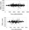 |
Fig. 1 Temporal variations of the astrometric shifts along (top) and perpendicular to (bottom) the equator, caused by the combination of spots and bright structures. The Sun is supposed to be seen edge-on and located 10 pc away. |
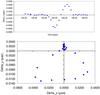 |
Fig. 2 Astrometric shift (deltax) as a function of time (top) and excursions of the photocenter (bottom) during a low-activity period (JD 2450335 to JD 2450365). |
Finally, we provide in Fig. 2 the temporal variations of the astrometric shift along the equator as well as the global excursion of the photocenter during a short 30-day period during the low-activity phase. The astrometric signal, if measured precisely enough, allows the determination of the star rotation period. The same is true for the RV and photomteric signals. The astrometric signal would furthermore provide additional and unique information. In Fig. 2, we see that the structure at the origin of the observed variations is located in the southern hemisphere of the star, and it moves from east to west, i.e. from the left to the right in the lower panel of Fig. 2. Therefore, the astrometric signal provides the means, within one rotation period, to determine the direction of the star’s rotational axis in the plane of the sky. Note that this assumes that we know by photometry or RV measurements if the perturbating structures are hotter or cooler than the photosphere and requires a very good astrometric precision. Moreover, one needs to isolate and monitor one single structure, which means that only periods of low activity can provide this information (indeed, during more active periods, the contributions of all individual structures mix).
Measured rms for the shifts, RV and photometry caused by the spots and bright structures.
2.3. Relation between RV, photometric, and astrometric signals
The astrometric variations along the equatorial plane are well correlated with the RV signal caused by spots and plages (see top panel of Fig. 3). For a single spot, the ratio between the shift and the RV depends on the star’s properties (vsini) and is almost independant of the spot properties. The correlation found here shows that this property remains when taking several spots/structures into account. The slope of the RV variations (in m/s) to the shifts (in μas) is 5, which is compatible with the value expected from a single spot. Once convection is taken into account in the RV computation, however, there is no correlation any longer between the astrometric shift in x and the RV variations (see Fig. 3). This difference of behaviour between the “no-convection” and “convection” cases could in principle be used to estimate the level of convection, if any, that is associated to the star.
Finally, no correlation is found between the relative photometric variations and the astrometric shifts (either the Δx or the shift-to-centre). This is not surprising because the photometric variations marginally depend on the spot/plage locations, conversely to the astrometric shifts.
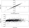 |
Fig. 3 Astrometric shifts along the equatorial plane versus RVs caused by spots and plages (top) and to spots, plages, and convection (bottom). No instrumental noise is assumed here. |
3. Discussion
3.1. Planet detection in astrometry
We see in Fig. 1 that the activity-induced shifts are most of the time smaller than 0.2 μas, i.e. smaller than the amplitude of the shifts induced by an Earth-mass planet at 1 AU (0.33 μasalong the equatioral plane and 0 μasperpendicular to the equator). These values agree with the estimates of Makarov et al. (2010). The rms of the equatorial shift over the entire cycle is about five times smaller than the amplitude of the Earth signal, and four times smaller during high activity. This means that the Sun activity would not prevent the detection of an Earth-like planet located in the HZ, provided the precision of the data allows for these mesurements. This is illustrated in Fig. 4, where we show the periodogram of the astrometric shifts along the equatorial plane once a one Earth-mass planet has been added (no noise). In this example, we use a limited amount of data instead of the whole set of data, in order to be closer to a real case. The chosen temporal sampling is of one month  five days over 50 months, which is typical of the strategy adopted for the NEAT instrument recently proposed to ESA (Léger 2010), dedicated to a systematic astrometric search for exo-Earths in the HZ of nearby stars.
We then explored different instrumental noises. An example is given in the lower panel of Fig. 4 where we assume a noise of 0.8 μas1. The temporal sampling is the same as before. The planet is still detectable. However, now the correlation seen in the previous section between the astrometric shift along the equatorial plane and the RV variations is not any longer present. This is because the instrumental noise exceeds the activity-induced noise. The consequence is that if we take the instrumental noise into account, it will not be possible with this level of activity to estimate the level of convection using the astrometric and RV data.
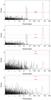 |
Fig. 4 Periodograms of the shift along the equatorial plane of the Sun viewed edge-on and surrounded by a one Earth-mass planets at 1AU, and observed once a month approximately, for 50 months. From top to bottom: 1) low-activity period, no instrumental noise; 2) high-activity period, no instrumental noise; 3) low-activity period, 0.8 μasrms instrumental noise; 4) high-activity period, 0.8 μasrms instrumental noise. |
We finally explore different levels of activity. We found that an instrumental precision similar to that expected for the NEAT instrument for a five hour-long visit of a G2 star located 10 pc away (0.35 μas) will easily allow the detection even for stars five times more active than the Sun (we conservatively assume that such a star will produce shifts five times higher than the Sun)2. This is illustrated in Fig. 5 where we show the periodograms of the shift along the equatorial plane (same sampling as before) during the low- and high-activity periods. Given Lockwood et al. (2007) relation between the relative photometric variations and the Ca H & K line strength index log(R’HK), and given the log(R’HK) for the Sun (between ≃ −4.85 and −5.0 respectively during the high- and low-activity phases), this corresponds to a log(R’HK) smaller than −4.25. Most active stars fall into this regime. Indeed, among the 385 Hipparcos stars closer than 20 pc with a known R’HK, only eight have log(R’HK) ≥ −4.2 (see Fig. 6; Maldonado et al. 2010).
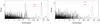 |
Fig. 5 Periodograms of the shift along the equatorial plane assuming a sun five times more active than observed, viewed edge-on and surrounded by a one-Earth-mass planet at 1 AU, and observed once a month approximately, for 50 months. A 0.35 μasrms instrumental noise was added to the data. Left: low-activity period; right: high-activity period. |
 |
Fig. 6 Histogram of log(R’HK) for all Hipparcos stars closer than 20 pc, with a known R’HK. |
So far we assumed that the angle of the planet orbit (supposedly identical to the equatorial plane) is known. For real observations though, this information will not be known a priori and the planet may orbit outside the star’s equatorial plane. It appears that even in the presence of stellar activity and instrumental noise at a level of 0.35 μasper measurement, the astrometric data will allow us to recover this information. We consider the example of a planet on an orbit inclined by −60 degrees with respect to the North. The star is supposed to have either the same activity level as our Sun, or five times this level. The astrometric shifts are measured in a reference frame that is allowed to rotate from 0 (equatorial plane) to 360 degrees. We measure in each case the shifts projected on this reference frame, and the associated rms along each axis of the reference frame. We consider either no or 0.35 μas level instrumental noise, and either a solar-like level of activity or five times this level. The temporal sampling is the same as before (50 data points). We show in Fig. 7 the rms as a function of the rotation angle of the reference frame. We see a clear maximum at an angle equal to the planet inclination. Hence the position angle of the planet orbit can be retrieved.
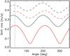 |
Fig. 7 Rms of the shift along the x-axis of a rotating reference frame as a function of its rotational angle (see text). In red, we show the case of solar activity. In blue, we show the case of five times the solar activity. In all cases, we consider that the instrumental noise is 0 (plain lines) or 0.35 microas (dashed lines). The vertical dashed line shows the angle of the inclination of the planet orbital plane. |
We conclude that in most cases, the stellar activity will not be the dominant factor for the planet detectability in astrometry. The dominant factor will rather be the instrumental precision. Note that if present, other larger planets will also induce noise, which is not considered in this paper, but the series of blind tests conducted to estimate the detection capabilities of Earth-like planets in multiple systems by space-borne astrometry (Traub et al. 2010) have shown that this noise can be well circumvented.
3.2. Comparison with RV data
The situation is then different from the RV data, because the rms of the RV caused by spots and bright structures only (i.e. convection not taken into account) during the entire
cycle, the low-activity period, and the high-activity period respectively are three, one and four times larger than the amplitude of the Earth RV signal (see Table 1). When we include convection, the corresponding ratios become 24, 4, and 14, respectively. Therefore, the RV detection limit is set by the stellar activity (and mainly by convection effects) rather than by the instrumental precision (provided precisions of 10 cm/s are available).
To prepare and accompany a space astrometric misson dedicated to Earth-mass planet detection, previous RV or photometric monitoring would certainly be very much appreciated. In particular, RV measurements are very powerful to derive the properties of the star’s activity. They are indeed more powerfull than astrometry, because the rms of the activity-induced RV variations is much larger than the instrumental precision (conversely to astrometry). Previous long-term RV monitoring can allow the identification of the presence of larger bodies in the system and characterize them (note that lower precision astrometric monitoring can also do this). During the astrometric measurements, simultaneous RV observations with a precision of about 10 cm/s would provide detailed information on the actual activity of the star and will help the analysis of the astrometric data.
This value corresponds to the precision that NEAT will provide in one hour observations. In practice, each visit will be longer (up to about five hours) to ensure a better precision (precision is proportional to  ).
).
In practice, a level of activity five times higher will probably induce shifts smaller than 5 times the shifts, as statistically, there will be more chances that the effects of structures located on a given side of the hemisphere be balanced by that those of structures on the opposite side
Acknowledgments
We acknowledge support from the French CNRS. We are grateful to Programme National de Planétologie (PNP, INSU). We also thank Alain Léger and Mike Shao for fruitfull discussions on the NEAT project and the referee for his prompt comments.
References
- Froehlich, C., & Lean, J. 1998, Geophys. Res. Lett., 25, 4377 [NASA ADS] [CrossRef] [Google Scholar]
- Lagrange, A.-M., Desort, M., & Meunier, N. 2010, A&A, 512, A38 [NASA ADS] [CrossRef] [EDP Sciences] [Google Scholar]
- Léger, A. 2010, priv. comm. [Google Scholar]
- Lockwood, G. W., Skiff, B. A., Henry, G. W., et al. 2007, ApJ, 171, L260 [Google Scholar]
- Makarov, V. V., Parker, D., & Ulrich, R. K. 2010, ApJ, 717, 1202 [NASA ADS] [CrossRef] [Google Scholar]
- Maldonado, J., Martínez-Arnáiz, R. M., Eiroa, C., Montes, D., & Montesinos, B. 2010, A&A, 521, A12 [NASA ADS] [CrossRef] [EDP Sciences] [Google Scholar]
- Meunier, N., Desort, M., & Lagrange, A.-M. 2010, A&A, 512, A39 [NASA ADS] [CrossRef] [EDP Sciences] [Google Scholar]
- Scherrer, P. H., Bogart, R. S., Bush, R. I., et al. 1995, Sol. Phys., 162,129 [Google Scholar]
- Traub, W., Beichman, C., Boden, A.F., et al. 2010, EAS Publi. Ser., 42,191 [CrossRef] [EDP Sciences] [Google Scholar]
All Tables
Measured rms for the shifts, RV and photometry caused by the spots and bright structures.
All Figures
|
Fig. 1 Temporal variations of the astrometric shifts along (top) and perpendicular to (bottom) the equator, caused by the combination of spots and bright structures. The Sun is supposed to be seen edge-on and located 10 pc away. |
| In the text | |
|
Fig. 2 Astrometric shift (deltax) as a function of time (top) and excursions of the photocenter (bottom) during a low-activity period (JD 2450335 to JD 2450365). |
| In the text | |
|
Fig. 3 Astrometric shifts along the equatorial plane versus RVs caused by spots and plages (top) and to spots, plages, and convection (bottom). No instrumental noise is assumed here. |
| In the text | |
|
Fig. 4 Periodograms of the shift along the equatorial plane of the Sun viewed edge-on and surrounded by a one Earth-mass planets at 1AU, and observed once a month approximately, for 50 months. From top to bottom: 1) low-activity period, no instrumental noise; 2) high-activity period, no instrumental noise; 3) low-activity period, 0.8 μasrms instrumental noise; 4) high-activity period, 0.8 μasrms instrumental noise. |
| In the text | |
|
Fig. 5 Periodograms of the shift along the equatorial plane assuming a sun five times more active than observed, viewed edge-on and surrounded by a one-Earth-mass planet at 1 AU, and observed once a month approximately, for 50 months. A 0.35 μasrms instrumental noise was added to the data. Left: low-activity period; right: high-activity period. |
| In the text | |
|
Fig. 6 Histogram of log(R’HK) for all Hipparcos stars closer than 20 pc, with a known R’HK. |
| In the text | |
|
Fig. 7 Rms of the shift along the x-axis of a rotating reference frame as a function of its rotational angle (see text). In red, we show the case of solar activity. In blue, we show the case of five times the solar activity. In all cases, we consider that the instrumental noise is 0 (plain lines) or 0.35 microas (dashed lines). The vertical dashed line shows the angle of the inclination of the planet orbital plane. |
| In the text | |
Current usage metrics show cumulative count of Article Views (full-text article views including HTML views, PDF and ePub downloads, according to the available data) and Abstracts Views on Vision4Press platform.
Data correspond to usage on the plateform after 2015. The current usage metrics is available 48-96 hours after online publication and is updated daily on week days.
Initial download of the metrics may take a while.