| Issue |
A&A
Volume 528, April 2011
|
|
|---|---|---|
| Article Number | A106 | |
| Number of page(s) | 19 | |
| Section | Numerical methods and codes | |
| DOI | https://doi.org/10.1051/0004-6361/201015630 | |
| Published online | 10 March 2011 | |
A fluid-dynamical subgrid scale model for highly compressible astrophysical turbulence
1
Institut für Astrophysik, Universität Göttingen,
Friedrich-Hund-Platz 1,
37077
Göttingen,
Germany
e-mail: schmidt@astro.physik.uni-goettingen.de
2
Zentrum für Astronomie der Universität Heidelberg, Institut für
Theoretische Astrophysik, Albert-Ueberle-Str. 2, 69120
Heidelberg,
Germany
e-mail: chfeder@ita.uni-heidelberg.de
3
Max-Planck-Institut für Astronomie, Königstuhl 17, 69117
Heidelberg,
Germany
4
École Normale Supérieure de Lyon, CRAL,
69364
Lyon Cedex 07,
France
Received:
24
August
2010
Accepted:
27
November
2010
Context. Compressible turbulence influences the dynamics of the interstellar and the intergalactic medium over a vast range of length scales. In numerical simulations, phenomenological subgrid scale (SGS) models are used to describe particular physical processes below the grid scale. In most cases, these models do not cover fluid-dynamical interactions between resolved and unresolved scales, or the employed SGS model is not applicable to turbulence in the highly compressible regime.
Aims. We formulate and implement the Euler equations with SGS dynamics and provide numerical tests of an SGS turbulence energy model that predicts the turbulent pressure of unresolved velocity fluctuations and the rate of dissipation for highly compressible turbulence.
Methods. We tested closures for the turbulence energy cascade by filtering data from high-resolution simulations of forced isothermal and adiabatic turbulence. Optimal properties and an excellent correlation are found for a linear combination of the eddy-viscosity closure that is employed in LES of weakly compressible turbulence and a term that is nonlinear in the Jacobian matrix of the velocity. Using this mixed closure, the SGS turbulence energy model is validated in LES of turbulence with stochastic forcing.
Results. It is found that the SGS model satisfies several important requirements: 1. The mean SGS turbulence energy follows a power law for varying grid scale. 2. The root mean square (rms) Mach number of the unresolved velocity fluctuations is proportional to the rms Mach number of the resolved turbulence, independent of the forcing. 3. The rate of dissipation and the turbulence energy flux are constant. Moreover, we discuss difficulties with direct estimates of the turbulent pressure and the dissipation rate on the basis of resolved flow quantities that have recently been proposed.
Conclusions. In combination with the energy injection by stellar feedback and other unresolved processes, the proposed SGS model is applicable to a variety of problems in computational astrophysics. By computing the SGS turbulence energy, the treatment of star formation and stellar feedback in galaxy simulations can be improved. Furthermore, we expect that the turbulent pressure on the grid scale affects the stability of gas against gravitational collapse. The influence of small-scale turbulence on emission line broadening, e.g., of O VI, in the intergalactic medium is another potential application.
Key words: hydrodynamics / turbulence / methods: numerical / ISM: kinematics and dynamics / galaxies: evolution
© ESO, 2011
1. Introduction
The effects of numerically unresolved turbulence have recently met increasing attention in a variety of astrophysical simulations (see, for instance, Scannapieco & Brüggen 2008; Maier et al. 2009; Joung et al. 2009; Oppenheimer & Davé 2009). Some approaches comprise subgrid scale (SGS) models, although these models are basically phenomenological parameterizations of astrophysical processes on length scales smaller than the grid scale. The full multi-scale dynamics of turbulence, however, is not embraced. The essence of an SGS model in the fluid-dynamical sense is that, at high Reynolds numbers, energy is transported through a turbulent cascade from larger, numerically resolved length scales to the subgrid scales. The energy of the unresolved turbulent velocity fluctuations is eventually dissipated into heat. Numerical simulations, in which an explicit closure for the turbulent cascade is applied on the grid scale, are called large eddy simulations (LES). A closure is an approximation to an SGS quantity in terms of resolved flow quantities.
If the unresolved turbulent velocity fluctuations reach a non-negligible fraction of the speed of sound, they give rise to a turbulent pressure in addition to the thermal pressure of the gas. This contribution to the pressure is proportional to the energy density of the SGS turbulence. Turbulent pressure effects in the baryonic gas component of star-forming galaxies are discussed in Burkert et al. (2010). In contemporary numerical simulations of disk galaxies (e.g., Dobbs et al. 2008; Tasker & Tan 2009; Agertz et al. 2009, 2010) or in galactic-scale simulations of the interstellar medium (e.g., Joung & Mac Low 2006; Joung et al. 2009), the minimal grid scale (or the SPH smoothing length) Δ ≳ 1 pc. Since this length scale is comparable to the size of molecular clouds, the unresolved turbulent velocity fluctuations can exceed the speed of sound in the cold-gas phase. Consequently, it can be expected that a significant turbulent pressure is caused by turbulence below the grid scale. To compute the turbulent pressure, which has an impact on the star formation rate through the stability of the gas against gravitational collapse, a model for the highly compressible regime is indispensable. Bonazzola et al. (1987) and Bonazzola et al. (1992) formulate an analytic theory to calculate the turbulent pressure of isotropic compressible turbulence on the integral length scale. By applying an SGS model, on the other hand, the turbulent pressure can be computed for any length scale within the inertial subrange. Joung et al. (2009) present an SGS model that is based on the equation for the kinetic energy of the unresolved turbulent velocity fluctuations, the so-called SGS turbulence energy, where energy is solely supplied by supernova feedback. Since the non-diagonal SGS turbulence stresses are neglected, the model of Joung et al. (2009) reduces the effects of SGS turbulence to the turbulent pressure alone, and the turbulence energy cascade, i.e., the production of SGS turbulence by the shear of the numerically resolved flow, is not considered.
Another example for this type of SGS models is the model of Scannapieco & Brüggen (2008) for the simulation of Rayleigh-Taylor-driven turbulence in active galactic nuclei, where it is assumed that SGS turbulence is produced by buoyancy processes only on unresolved length scales. These processes are modelled by an equation for the characteristic length scale of the Rayleigh-Taylor instability. In contrast, Schmidt et al. (2006b) incorporate unresolved buoyancy effects into an SGS model that includes the production by shear for the treatment of turbulent combustion in thermonuclear supernovae.
In the cosmological simulations of galaxy clusters by Maier et al. (2009), the role of SGS turbulence has been explored with a numerical technique that combines adaptive mesh refinement and LES. They apply the SGS turbulence energy model of Schmidt et al. (2006a). The main effect of the SGS model is an enhancement of the turbulent heating in the cluster core. The SGS turbulence energy also serves as a tracer of turbulence production in the intergalactic medium (Iapichino et al. 2011). However, a deficiency in these simulations is that the employed SGS model is only applicable to moderately compressible turbulence. Shocks are treated tentatively, i.e., SGS turbulence production is suppressed in the vicinity of shock fronts. While this is not a severe constraint for the bulk of the intracluster medium, in which the Mach numbers of the turbulent flow are small compared to unity, an erroneous production of SGS turbulence energy is likely to occur near accretion shocks in the outer regions of the cluster.
In this article, we improve on the previous approaches to SGS modelling by addressing the closure problem for highly compressible turbulence. In Sect. 2, we discuss the meaning of the compressible Euler equations in the context of computational fluid dynamics. The verification of the proposed closure and the calibration of the closure coefficients are presented in Sect. 3. Data from several high-resolution simulations of forced turbulence (Schmidt et al. 2007, 2009; Federrath et al. 2010b) allow us to compute the rate at which energy is transferred from length scales greater than the filter length to smaller length scales and to test the correlation with different closures. As a result, we propose a combination of the eddy-viscosity closure, which has been used successfully in LES of incompressible turbulence, and a nonlinear closure put forward by Woodward et al. (2006). Then we show that physically reasonable statistics of the SGS turbulence energy and the rate of dissipation are obtained for varying grid resolutions and forcing in LES of supersonic turbulence (Sect. 4). Furthermore, we investigate correlations of the SGS quantities with quantities derived from the numerically resolved flow. We demonstrate that the turbulent pressure and energy dissipation cannot be predicted in a straightforward way on the basis of the resolved turbulent flow, as proposed, for instance, by Pan et al. (2009) and Zhu et al. (2010). Instead, a full SGS model is needed to estimate unresolved turbulence effects. In the last section, we summarize the results and discuss potential astrophysical applications of the closure for the highly compressible turbulent cascade in combination with the phenomenological approaches described above.
2. The compressible Euler equations with subgrid-scale dynamics
The Reynolds number of turbulent flows in astrophysics is usually considered to be high
enough so that the approximation of an inviscid fluid can be applied on numerically
resolvable length scales. For a physically complete picture, we begin with the compressible
Navier-Stokes equations encompassing all physical length scales. This acknowledges that
perfect fluids do not exist in nature and that the notion of viscous dissipation is
essential for turbulence. The fluid-dynamical variables determined by this set of equations
are denoted by  for the mass density of
the gas,
for the mass density of
the gas,  for the velocity of
the flow, etc.1. The resolution of a numerical
simulation is given by the size of the grid cells Δ, which is called the cutoff scale or the
grid scale. A consistent formulation of the equations of fluid dynamics with a cutoff scale
Δ can by derived from the Navier-Stokes equations by means of the filter formalism
introduced by Germano (1992). Generalizing this
formalism to compressible fluid dynamics is straightforward (see Schmidt et al. 2006a). The basic idea is to identify the numerically
computed solution with filtered variables
for the velocity of
the flow, etc.1. The resolution of a numerical
simulation is given by the size of the grid cells Δ, which is called the cutoff scale or the
grid scale. A consistent formulation of the equations of fluid dynamics with a cutoff scale
Δ can by derived from the Navier-Stokes equations by means of the filter formalism
introduced by Germano (1992). Generalizing this
formalism to compressible fluid dynamics is straightforward (see Schmidt et al. 2006a). The basic idea is to identify the numerically
computed solution with filtered variables  ,
,
 , etc. The filter operator
⟨ · ⟩ Δ smooths the physical variables that are given by the Navier-Stokes
equations over the length scale Δ. In LES, the filtering corresponds to the discretization
of the equations of fluid dynamics. The dynamical equations for the computable, filtered
quantities are similar to the unfiltered equations, with additional terms that are related
to the subgrid-scale dynamics on length scales
ℓ < Δ.
, etc. The filter operator
⟨ · ⟩ Δ smooths the physical variables that are given by the Navier-Stokes
equations over the length scale Δ. In LES, the filtering corresponds to the discretization
of the equations of fluid dynamics. The dynamical equations for the computable, filtered
quantities are similar to the unfiltered equations, with additional terms that are related
to the subgrid-scale dynamics on length scales
ℓ < Δ.
Let us consider the dynamical equation for the momentum density of the fluid, which is
given by the partial differential equation (PDE) 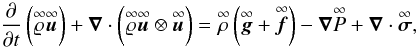 (1)where
 and
and
 are the accelerations
due to gravity and other mechanical forces acting on the fluid, and
are the accelerations
due to gravity and other mechanical forces acting on the fluid, and
 is the thermal
pressure. The viscous dissipation tensor
is the thermal
pressure. The viscous dissipation tensor  is defined by
 (2)where
ν is the microscopic viscosity of the fluid2, the rate of strain
(2)where
ν is the microscopic viscosity of the fluid2, the rate of strain  is the symmetic
part of the Jacobian matrix
is the symmetic
part of the Jacobian matrix  , and
, and
 . After applying a
homogeneous filter operator that is uniform in time, Eq. (1) is converted into an equation for the filtered momentum,
. After applying a
homogeneous filter operator that is uniform in time, Eq. (1) is converted into an equation for the filtered momentum,
 . This
equation has the same form as the original equation, except for one term. Because of the
nonlinear advection term, the filtering introduces a stress term that accounts for the
interaction between the numerically resolved flow and velocity fluctuations on the subgrid
scales:
. This
equation has the same form as the original equation, except for one term. Because of the
nonlinear advection term, the filtering introduces a stress term that accounts for the
interaction between the numerically resolved flow and velocity fluctuations on the subgrid
scales: 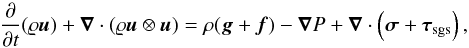 (3)where the SGS
turbulence stress tensor is defined by
(3)where the SGS
turbulence stress tensor is defined by  (4)In the following, the
components of τsgs are simply denoted by
τij. The second-order moment
(4)In the following, the
components of τsgs are simply denoted by
τij. The second-order moment
 is not explicitly
computable in LES because the variations in the mass density
and the velocity
below the grid
scale are unknown. For this reason, an approximation in terms of filtered quantities has to
be devised. This is the closure problem3.
is not explicitly
computable in LES because the variations in the mass density
and the velocity
below the grid
scale are unknown. For this reason, an approximation in terms of filtered quantities has to
be devised. This is the closure problem3.
The SGS turbulence energy density is defined by the difference between the resolved kinetic
energy and the filtered kinetic energy: 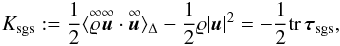 (5)where
tr τsgs = τii
is the trace of the SGS turbulence stress tensor. One can see that the trace of
τsgs gives rise to the term
(5)where
tr τsgs = τii
is the trace of the SGS turbulence stress tensor. One can see that the trace of
τsgs gives rise to the term
 on the right
hand side of Eq. (3). This term can be
absorbed into the pressure gradient if the thermal pressure P is replaced
by the effective pressure
on the right
hand side of Eq. (3). This term can be
absorbed into the pressure gradient if the thermal pressure P is replaced
by the effective pressure  (6)The relative
contribution of the turbulent pressure
(6)The relative
contribution of the turbulent pressure  compared to the
thermal pressure P is characterized by the SGS turbulence Mach number
compared to the
thermal pressure P is characterized by the SGS turbulence Mach number
 ,
where cs is the thermal speed of sound. ℳsgs depends
on the temperature of the fluid and the cutoff scale Δ. The dependence on Δ is investigated
in Sect. 4.2. Joung
et al. (2009) define the turbulent pressure by
Psgs = (γ − 1)Ksgs,
where γ is the adiabatic coefficient of the gas. We emphasize that, except
for γ = 5/3, this definition is inconsistent with the
decomposition of the fluid-dynamical equations, which fixes the coefficient to
2/3 (see also Chandrasekhar
1951). This is reasonable because the turbulent pressure is solely a property of the
turbulent flow of a gas on a given length scale, whereas γ is a microscopic
property of the gas that is related to the thermal motions of the atoms or molecules.
,
where cs is the thermal speed of sound. ℳsgs depends
on the temperature of the fluid and the cutoff scale Δ. The dependence on Δ is investigated
in Sect. 4.2. Joung
et al. (2009) define the turbulent pressure by
Psgs = (γ − 1)Ksgs,
where γ is the adiabatic coefficient of the gas. We emphasize that, except
for γ = 5/3, this definition is inconsistent with the
decomposition of the fluid-dynamical equations, which fixes the coefficient to
2/3 (see also Chandrasekhar
1951). This is reasonable because the turbulent pressure is solely a property of the
turbulent flow of a gas on a given length scale, whereas γ is a microscopic
property of the gas that is related to the thermal motions of the atoms or molecules.
The SGS turbulence energy is an intermediate reservoir of energy that exchanges energy with
the resolved flow and loses energy by dissipation into heat. For the computation of
Ksgs, a PDE has to be solved in addition to the filtered
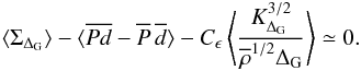
equations for the resolved gas dynamics:  (7)While
Σ = τijSij
is the rate of SGS turbulence energy production by the turbulent cascade through the cutoff
scale Δ (also called the turbulence energy flux) and ρϵ is the viscous
dissipation rate smoothed over Δ, effects caused by SGS fluctuations of the gravitational
potential and the thermal pressure are given by Γ and ρλ, respectively. The
term D accounts for SGS transport effects. We refer to Schmidt et al. (2006a), Eqs. (33)–(37), for the exact definitions of these terms.
For our purpose it is sufficient to discuss the closures of these terms, which are
approximations in terms of the numerically resolved variables and
Ksgs.
(7)While
Σ = τijSij
is the rate of SGS turbulence energy production by the turbulent cascade through the cutoff
scale Δ (also called the turbulence energy flux) and ρϵ is the viscous
dissipation rate smoothed over Δ, effects caused by SGS fluctuations of the gravitational
potential and the thermal pressure are given by Γ and ρλ, respectively. The
term D accounts for SGS transport effects. We refer to Schmidt et al. (2006a), Eqs. (33)–(37), for the exact definitions of these terms.
For our purpose it is sufficient to discuss the closures of these terms, which are
approximations in terms of the numerically resolved variables and
Ksgs.
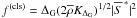
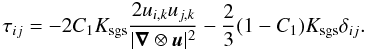
To compute the SGS turbulence stress tensor (4), we propose the following closure for the highly compressible regime:
 (8)where
|∇ ⊗ u|: = (2ui,kui,k)1/2
is the norm of the resolved velocity derivative,
(8)where
|∇ ⊗ u|: = (2ui,kui,k)1/2
is the norm of the resolved velocity derivative,  is the trace-free
part of
is the trace-free
part of  , and
d = ui,i. While the first
term in Eq. (8) corresponds to the
eddy-viscosity closure that is commonly used in incompressible LES, the second, nonlinear
term was investigated by Woodward et al. (2006) for
transonic decaying turbulence. The standard eddy-viscosity closure follows if
C2 = 0. In general, the linear eddy-viscosity term dominates
if
(Ksgs/ρ)1/2
is small compared to
Δ|S∗| ≲ Δ|∇ ⊗ u|. On
the other hand, for strong turbulence intensity, i.e.,
(Ksgs/ρ)1/2 ≳ Δ|∇ ⊗ u|,
the nonlinear term contributes significantly. This particularly applies to intermittent
events in supersonic turbulence, for which
Δ|∇ ⊗ u| ≳ cs.
In moderately compressible turbulence, nonlinear contributions affect the high-intermittency
tails of the turbulent energy distribution. Independent of the values of
C1 and C2,
τii = −2Ksgs,
as required by the identity (5). We denote
the trace-free part of the SGS turbulence stress tensor by
, and
d = ui,i. While the first
term in Eq. (8) corresponds to the
eddy-viscosity closure that is commonly used in incompressible LES, the second, nonlinear
term was investigated by Woodward et al. (2006) for
transonic decaying turbulence. The standard eddy-viscosity closure follows if
C2 = 0. In general, the linear eddy-viscosity term dominates
if
(Ksgs/ρ)1/2
is small compared to
Δ|S∗| ≲ Δ|∇ ⊗ u|. On
the other hand, for strong turbulence intensity, i.e.,
(Ksgs/ρ)1/2 ≳ Δ|∇ ⊗ u|,
the nonlinear term contributes significantly. This particularly applies to intermittent
events in supersonic turbulence, for which
Δ|∇ ⊗ u| ≳ cs.
In moderately compressible turbulence, nonlinear contributions affect the high-intermittency
tails of the turbulent energy distribution. Independent of the values of
C1 and C2,
τii = −2Ksgs,
as required by the identity (5). We denote
the trace-free part of the SGS turbulence stress tensor by
 . The
verification of the generalized closure (8)
for τij and the determination of the
coefficients C1 and C2 for
supersonic turbulence is the key to computing the turbulent pressure
, as
Ksgs first and foremost depends on the production rate
Σ = τijSij
in Eq. (7).
. The
verification of the generalized closure (8)
for τij and the determination of the
coefficients C1 and C2 for
supersonic turbulence is the key to computing the turbulent pressure
, as
Ksgs first and foremost depends on the production rate
Σ = τijSij
in Eq. (7).
Due to the microscopic viscosity ν of the fluid, the viscous stresses
 dissipate
kinetic energy on the smallest dynamical length scales
ℓ ~ η of the physical flow
dissipate
kinetic energy on the smallest dynamical length scales
ℓ ~ η of the physical flow
 . The length scale
η is called the Kolmogorov scale. In the filtered momentum Eq. (3), viscous dissipation effects are given by the
divergence of the filtered tensor
. The length scale
η is called the Kolmogorov scale. In the filtered momentum Eq. (3), viscous dissipation effects are given by the
divergence of the filtered tensor  . The corresponding rate
of energy dissipation, filtered on the grid scale, is given by
. The corresponding rate
of energy dissipation, filtered on the grid scale, is given by  (9)It is important to
note that
ϱϵ ≠ σijui,j,
where σij and
ui,j are the filtered viscous stress tensor
and the filtered velocity gradient, respectively.
(9)It is important to
note that
ϱϵ ≠ σijui,j,
where σij and
ui,j are the filtered viscous stress tensor
and the filtered velocity gradient, respectively.
For fully developed incompressible turbulence, the Kolmogorov scale can be related to the Reynolds number: η/L ~ Re3/4, where Re: = VL/ν for an integral length L and characteristic velocity V of the flow. As pointed out at the beginning of this section, Re is assumed to be very high in astrophysical systems. In this case, η is much smaller than any feasible grid resolution Δ, and simple scaling arguments show that the viscous stress term in the filtered momentum Eq. (3) is negligible (Röpke & Schmidt 2009), i.e., |σ| ≪ |τsgs|. Consequently, the physical energy dissipation occurs entirely on subgrid scales ℓ ≪ Δ. As η decreases in comparison to Δ, the velocity fluctuations on ever smaller length scales give rise to arbitrarily steep velocity gradients, which add up to a non-vanishing product of the viscosity times the squared rate of strain on the right hand side of Eq. (9), regardless of how small the viscosity is. This results in a non-zero, asymptotically constant mean rate of energy dissipation in the limit η → 0 (ν → 0), which is supported by experimental and numerical evidences (see Frisch 1995; Ishihara et al. 2009). We may reasonably conjecture that the viscous dissipation tensor is negligible in the filtered momentum equation and the energy dissipation rate does not vanish in the limit of infinite Reynolds numbers also in the case of compressible turbulence. A posteriori tests imply that this conjecture is fulfiled for driven supersonic turbulence (see Sect. 4.2). However, the question of energy dissipation in inhomogeneous turbulence is more difficult. For example, it is known from boundary layers of terrestrial turbulence that viscous effects can affect the flow on relatively large scales near a wall. For this reason, the microscopic viscosity cannot be neglected in LES of such flows. Although solid walls are not encountered in astrophysics, many relevant problems exhibit pronounced inhomogeneities, and we cannot entirely exclude the possibility that viscous effects might become noticeable on resolved length scales in certain cases.
A closure for ϵ follows from simple dimensional reasoning:  (10)Here, it is assumed that
the SGS turbulence energy is dissipated into heat at a rate proportional to
Ksgs divided by the time scale
Δ(Ksgs/ρ)−1/2.
For the pressure-dilatation term ρλ several closures have been proposed
(e.g., Sarkar 1992; Fureby et al. 1997). However, applying a priori tests (see Sect. 3), we find that these closures clearly fail in the case of
supersonic turbulence. The simplest solution is to neglect pressure dilatation entirely
(Woodward et al. 2006). In this article, we also
set ρλ = 0, although we are aware that pressure-dilatation effects have
potential significance, particularly in the case of adiabatic turbulence. The transport term
in Eq. (7) can be modelled by a
gradient-diffusion approximation (see Sagaut 2006):
(10)Here, it is assumed that
the SGS turbulence energy is dissipated into heat at a rate proportional to
Ksgs divided by the time scale
Δ(Ksgs/ρ)−1/2.
For the pressure-dilatation term ρλ several closures have been proposed
(e.g., Sarkar 1992; Fureby et al. 1997). However, applying a priori tests (see Sect. 3), we find that these closures clearly fail in the case of
supersonic turbulence. The simplest solution is to neglect pressure dilatation entirely
(Woodward et al. 2006). In this article, we also
set ρλ = 0, although we are aware that pressure-dilatation effects have
potential significance, particularly in the case of adiabatic turbulence. The transport term
in Eq. (7) can be modelled by a
gradient-diffusion approximation (see Sagaut 2006):
![\begin{equation} \mathfrak{D} = \vect{\nabla}\cdot\left[\kappa_{\mathrm{sgs}} \vect{\nabla}\left(\frac{K_{\mathrm{sgs}}}{\rho}\right)\right], \end{equation}](/articles/aa/full_html/2011/04/aa15630-10/aa15630-10-eq81.png) (11)where the SGS turbulent
diffusivity is approximated by
κsgs ≈ 0.65Δ(ρKsgs)1/2,
as shown by Schmidt et al. (2006a).
(11)where the SGS turbulent
diffusivity is approximated by
κsgs ≈ 0.65Δ(ρKsgs)1/2,
as shown by Schmidt et al. (2006a).
In this work, we assume that self-gravity has no significant effects on length scales
ℓ ≲ Δ. This corresponds to the condition that the local Jeans length
λ = cs(π/Gρ)1/2,
where G is the gravitational constant, is sufficiently large compared to
the grid scale Δ (Truelove et al. 1997; Federrath et al. 2010a). Thus, setting Γ = 0, the
filtered equations resulting from the compressible Navier-Stokes equations in the limit of
η ≪ Δ (Schmidt et al. 2006a) read
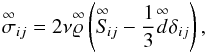
as ![\begin{align} \label{eq:euler_sgs_rho} \frac{\partial}{\partial t}\varrho + \vec{\nabla}\cdot(\vec{u}\varrho)\, &= 0, \\ \label{eq:euler_sgs_momt} \frac{\partial}{\partial t}(\varrho\vec{u}) + \vec{\nabla}\cdot\left(\varrho\vec{u}\otimes\vec{u}\right)\, &= \rho(\vect{g} + \vect{f}) -\vec{\nabla}(P + P_{\mathrm{sgs}}) + \vec{\nabla}\cdot\boldsymbol{\tau}_{\mathrm{sgs}}^{\ast}, \\ \begin{split} \label{eq:euler_sgs_energy} \frac{\partial}{\partial t} E + \vec{\nabla}\cdot(\vec{u}E)\, &= -\mathcal{L} + \rho\vect{u}\cdot(\vect{g} + \vect{f}) -\vec{\nabla}\cdot[\vec{u}(P + P_{\mathrm{sgs}})] \\ &+ \vec{\nabla}\cdot(\vec{u}\cdot\boldsymbol{\tau}_{\mathrm{sgs}}^{\ast}) - \Sigma + \rho\epsilon, \end{split} \end{align}](/articles/aa/full_html/2011/04/aa15630-10/aa15630-10-eq88.png) where
where
 is the sum of the
resolved kinetic and internal energy density, and −ℒ accounts for sources and sinks of the
internal energy due to heating and cooling, respectively. Since the resolved fluid dynamics
on length scales ℓ ≥ Δ is unaffected by the viscosity of the fluid, the
above set of equations defines the compressible Euler equations for
computational fluid dynamics in a physically meaningful and consistent way. These equations
are supplemented by an equation of state, the SGS turbulence energy Eq. (7), and the Poisson equation for the
gravitational potential. The pure compressible Euler equations without SGS terms, on the
other hand, do not follow from the compressible Navier-Stokes equation in
the limit of infinite Reynolds number. In this case, there is no viscous dissipation at all,
and, by definition, ϵ vanishes identically. This is a mathematical
idealization that does not describe turbulent flows in nature.
is the sum of the
resolved kinetic and internal energy density, and −ℒ accounts for sources and sinks of the
internal energy due to heating and cooling, respectively. Since the resolved fluid dynamics
on length scales ℓ ≥ Δ is unaffected by the viscosity of the fluid, the
above set of equations defines the compressible Euler equations for
computational fluid dynamics in a physically meaningful and consistent way. These equations
are supplemented by an equation of state, the SGS turbulence energy Eq. (7), and the Poisson equation for the
gravitational potential. The pure compressible Euler equations without SGS terms, on the
other hand, do not follow from the compressible Navier-Stokes equation in
the limit of infinite Reynolds number. In this case, there is no viscous dissipation at all,
and, by definition, ϵ vanishes identically. This is a mathematical
idealization that does not describe turbulent flows in nature.
As a special case, implicit large eddy simulations (ILES) follow from the
above approach. ILES is the most commonly used method in astrophysical fluid dynamics. It is
based on two assumptions, which are usually not stated in the literature. First, the
discretization of the compressible Euler equations introduces a dissipative leading error
term Dnum in the momentum Eq. (11). Implicitly, this term is assumed to be equivalent to the SGS turbulence stress
term ∇·τsgs. The second
assumption in ILES is that
u·Dnum = −ρϵ, i.e., kinetic
energy on the resolved scales is directly dissipated into heat at a rate that approximates
the viscous dissipation on unresolved length scales. This is referred to as numerical
viscosity or numerical dissipation. Actually, the following equations are solved in ILES:
 Despite
the lack of a mathematical justification, ILES serves as an approximation of turbulent
compressible fluid dynamics that has proven its utility in numerous astrophysical
applications. Benzi et al. (2008) demonstrate that the
ILES approach closely reproduces two-point statistics of weakly compressible turbulence in
the inertial subrange in comparison to direct numerical simulations that solve the
Navier-Stokes equations. In this article, we make use of ILES to compute high-resolution
data for the explicit verification of SGS closures. In contrast, LES treat the energy
dissipation explicitly. However, it cannot be avoided that numerical schemes for
compressible fluid dynamics such as the piecewise parabolic method (PPM, Colella & Woodward 1984) introduce some numerical
dissipation. Thus, by running an LES with an explicit SGS model, there is inevitably a
numerical dissipation channel that competes with the transfer of energy to the subgrid
scales and the subsequent dissipation of SGS turbulence energy into heat. Notwithstanding
this caveat, we demonstrate in this article that physically sensible predictions can by made
by an explicit SGS model, which are not possible on the basis of ILES.
Despite
the lack of a mathematical justification, ILES serves as an approximation of turbulent
compressible fluid dynamics that has proven its utility in numerous astrophysical
applications. Benzi et al. (2008) demonstrate that the
ILES approach closely reproduces two-point statistics of weakly compressible turbulence in
the inertial subrange in comparison to direct numerical simulations that solve the
Navier-Stokes equations. In this article, we make use of ILES to compute high-resolution
data for the explicit verification of SGS closures. In contrast, LES treat the energy
dissipation explicitly. However, it cannot be avoided that numerical schemes for
compressible fluid dynamics such as the piecewise parabolic method (PPM, Colella & Woodward 1984) introduce some numerical
dissipation. Thus, by running an LES with an explicit SGS model, there is inevitably a
numerical dissipation channel that competes with the transfer of energy to the subgrid
scales and the subsequent dissipation of SGS turbulence energy into heat. Notwithstanding
this caveat, we demonstrate in this article that physically sensible predictions can by made
by an explicit SGS model, which are not possible on the basis of ILES.
3. Closure verification
To test different closures for the turbulence energy flux Σ, we apply the method described in Schmidt et al. (2006a). The basic idea is to use data from ILES of non-selfgravitating isothermal and adiabatic turbulence with high numerical resolution and to apply an explicit filter to these data on a length scale that is in between the forcing and the dissipative range. The applied filters are Gaussian with filter lengths ΔG = 24Δ and 32Δ for 7683 and 10243 grids, respectively. Although the bottleneck effect has some influence on the chosen length scales (Schmidt et al. 2009; Federrath et al. 2010b), we show that the results change only slightly if the filter length decreases or increases by a factor of two. Moreover, comparing to box filters, the results turn out to be rather insensitive to the filter type.
3.1. Single-coefficient closures for supersonic isothermal turbulence
The turbulence energy flux on the filter scale ΔG can be computed explicitly
from the unfiltered numerical data by the formula  (18)where the first factor on
the right hand side is the turbulence stress tensor on the filter scale (defined analogous
to Eq. (4)) and the second factor is the
derivative of the filtered velocity. As a shorthand notation, we denote the explicitly
filtered quantities by an overline, for instance,
(18)where the first factor on
the right hand side is the turbulence stress tensor on the filter scale (defined analogous
to Eq. (4)) and the second factor is the
derivative of the filtered velocity. As a shorthand notation, we denote the explicitly
filtered quantities by an overline, for instance,  , and
, and
 .
.
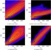 |
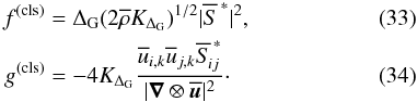
Fig. 1 Correlation diagrams for the SGS turbulence energy flux in the case of isothermal supersonic turbulence with solenoidal forcing (ℳrms ≈ 5.3). The applied filter length is 32Δ. The blue dots indicate the average prediction of the closure for a given value of Σ32Δ. |
The above expression for ΣΔG can be compared to closures. For the
eddy-viscosity closure, ΣΔG is given by 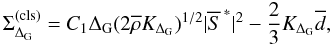 (19)where
 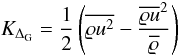 (20)is
the turbulence energy on length scales smaller than ΔG. Strictly speaking,
KΔG is the turbulence energy for the length
scales ranging from the grid resolution Δ to the smoothing length ΔG of the
Gaussian filter. If ΔG is sufficiently larger than Δ, this distinction can be
neglected (see Schmidt et al. 2006a).
(20)is
the turbulence energy on length scales smaller than ΔG. Strictly speaking,
KΔG is the turbulence energy for the length
scales ranging from the grid resolution Δ to the smoothing length ΔG of the
Gaussian filter. If ΔG is sufficiently larger than Δ, this distinction can be
neglected (see Schmidt et al. 2006a).
When defining 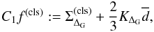 (21)the squared error
function of the closure can be written as
(21)the squared error
function of the closure can be written as
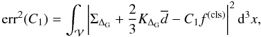 (22)where
ΣΔG and KΔG are given by
Eqs. (18) and (20), respectively, and the volume integral
extends over the whole domain
(22)where
ΣΔG and KΔG are given by
Eqs. (18) and (20), respectively, and the volume integral
extends over the whole domain  .
The minimum of err2(C1) yields the least squares
error solution for the closure coefficient,
.
The minimum of err2(C1) yields the least squares
error solution for the closure coefficient, ![\begin{equation} \label{eq:coeff_lse} C_{1}=\frac{\int_{\mathcal{V}} f^{(\rm cls)}\left[\Sigma_{\Delta_{\mathrm{G}}}+\frac{2}{3}K_{\Delta_{\rm G}}\overline{d}\right]\,\dd^{3}x}{\int_{\mathcal{V}} |f^{(\rm cls)}|^2\dd^{3}x}, \end{equation}](/articles/aa/full_html/2011/04/aa15630-10/aa15630-10-eq116.png) (23)where
(23)where
 for the
eddy-viscosity closure. For statistically stationary and isotropic turbulence, the closure
coefficient C1 is independent of the filter length scale
because of the local equilibrium of the transfer of turbulence energy in the inertial
subrange. Thus, the value of C1 inferred from Eq. (23) is an approximation to the coefficient of
the SGS closure for Σ in LES.
for the
eddy-viscosity closure. For statistically stationary and isotropic turbulence, the closure
coefficient C1 is independent of the filter length scale
because of the local equilibrium of the transfer of turbulence energy in the inertial
subrange. Thus, the value of C1 inferred from Eq. (23) is an approximation to the coefficient of
the SGS closure for Σ in LES.
To calculate C1, we use data from two 10243
simulations of supersonic isothermal turbulence with a root-mean-square (RMS) Mach number
around 5.5 (Federrath et al. 2010b). Statistically
stationary and isotropic turbulence is produced by stochastic forcing. Solenoidal
(divergence-free) forcing is applied in one simulation, while the forcing is compressive
(rotation-free) in the other simulation. We choose ΔG = 32Δ for the filtering
of the simulation data. Figures 1 and 2 show the correlation between
 and
ΣΔG by means of two-dimensional probability density functions.
For the eddy-viscosity closure (19), the
correlation is quite good (the spacing of the contour lines in Figs. 1 and 2 is logarithmic in the
two-dimensional probability density), but there is a problem with negative flux values.
The values of the closure coefficient C1 following from
Eq. (23) are listed in Table 1. Also listed are the correlation coefficients
and
ΣΔG by means of two-dimensional probability density functions.
For the eddy-viscosity closure (19), the
correlation is quite good (the spacing of the contour lines in Figs. 1 and 2 is logarithmic in the
two-dimensional probability density), but there is a problem with negative flux values.
The values of the closure coefficient C1 following from
Eq. (23) are listed in Table 1. Also listed are the correlation coefficients
![\begin{eqnarray} \mathrm{corr} &[\Sigma_{\Delta_{\rm G}},\Sigma_{\Delta_{\rm G}}^{(\rm cls)}] =\nonumber\\ &\frac{\int_{\mathcal{V}} \left[\Sigma_{\Delta_{\rm G}}-\langle\Sigma_{\Delta_{\rm G}}\rangle\right] \left[\Sigma_{\Delta_{\rm G}}^{(\rm cls)}-\langle\Sigma_{\Delta_{\rm G}}^{(\rm cls)}\rangle\right]\,\dd^{3}x}{\mathrm{std}[\Sigma_{\Delta_{\rm G}}]\mathrm{std}[\Sigma_{\Delta_{\rm G}}^{(\rm cls)}]}, \end{eqnarray}](/articles/aa/full_html/2011/04/aa15630-10/aa15630-10-eq122.png) (24)where
std [·] denotes the standard deviation and the angle brackets indicate an average over
the whole domain.
(24)where
std [·] denotes the standard deviation and the angle brackets indicate an average over
the whole domain.
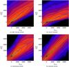 |
Fig. 2 Correlation diagrams for isothermal supersonic turbulence with compressive forcing (ℳrms ≈ 5.6) as in Fig. 1. |
An important question for the LES of supersonic turbulence is whether shocks can be
accommodated in closures for the turbulence energy. Since the eddy-viscosity closure
originates from incompressible turbulence, Maier et al.
(2009) suggests setting Σ equal to zero in the vicinity of shock fronts. This
should suppress the spurious production of SGS turbulence energy by the large strain at
shock fronts. Thus, we tested whether excluding shocks in the computation of the
eddy-viscosity closure for the turbulence energy flux would improve the correlations.
However, panels (b) in Figs. 1 and 2 make it clear that such a cutoff deteriorates the
correlations and implies a significant underestimate of large positive fluxes. Although
the applied shock detection criterion  is rather crude, we
interpret this trend as an indication that shocks must not be separated from the
supersonic turbulent cascade.
is rather crude, we
interpret this trend as an indication that shocks must not be separated from the
supersonic turbulent cascade.
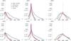 |
Fig. 3 Slices of the two-dimensional probability density functions plotted in Figs. 1 and 2, showing the predictions of different closures for the values of the explicitly computed energy flux Σ32Δ that are indicated by the vertical dashed lines. The top and bottom rows of panels show the results for solenoidal and compressive forcing, respectively. |
In addition to the conventional eddy-viscosity closure, we investigate a closure that is
based on the determinant of the velocity gradient (Woodward et al. 2001). In this case, the trace-free part of the SGS turbulence
stress tensor is still given by the expression  . The eddy
viscosity, however, does not depend on Ksgs, but is defined by
νsgs = −C1Δ2|S∗|−2detS∗.
Hence, the turbulence energy flux on the filter scale is given by
. The eddy
viscosity, however, does not depend on Ksgs, but is defined by
νsgs = −C1Δ2|S∗|−2detS∗.
Hence, the turbulence energy flux on the filter scale is given by  (25)for
this closure. Woodward et al. (2001) employ the
same method as we do to test the correlation between their closure and the turbulence
energy flux. A particularly interesting feature of the determinant is that it switches
signs, thereby describing two different flow topologies. In one case, the determinant is
negative. This corresponds to the forward turbulent cascade transporting energy from large
to smaller eddies. In the other case, the flow is contracting in one dimension and
expanding in the other two. Then the determinant is positive, corresponding to a
backscattering of energy from small to larger eddies. This phenomenon can be explained by
the alignment of vortices along a single stretching direction (the “tornado" topology).
While an energy flux of the form (19)
fails to describe the reverse cascade, we see in panels (c) of Figs. 1 and 2 that the determinant
closure yields a good correlation for negative energy flux. However, the overall
correlation does not significantly improve (see Table 1), because of the relatively large scatter in the forward cascade.
(25)for
this closure. Woodward et al. (2001) employ the
same method as we do to test the correlation between their closure and the turbulence
energy flux. A particularly interesting feature of the determinant is that it switches
signs, thereby describing two different flow topologies. In one case, the determinant is
negative. This corresponds to the forward turbulent cascade transporting energy from large
to smaller eddies. In the other case, the flow is contracting in one dimension and
expanding in the other two. Then the determinant is positive, corresponding to a
backscattering of energy from small to larger eddies. This phenomenon can be explained by
the alignment of vortices along a single stretching direction (the “tornado" topology).
While an energy flux of the form (19)
fails to describe the reverse cascade, we see in panels (c) of Figs. 1 and 2 that the determinant
closure yields a good correlation for negative energy flux. However, the overall
correlation does not significantly improve (see Table 1), because of the relatively large scatter in the forward cascade.
In Woodward et al. (2006), a nonlinear expression
for the turbulence stress tensor is investigated, which depends on the full Jacobian
∇ ⊗ u of the velocity:
 (26)Since
|∇ ⊗ u| = (2ui,kui,k)1/2,
the above expression fulfills the identity
τii = −2Ksgs.
The corresponding turbulence energy flux on the filter length scale ΔG is given
by
(26)Since
|∇ ⊗ u| = (2ui,kui,k)1/2,
the above expression fulfills the identity
τii = −2Ksgs.
The corresponding turbulence energy flux on the filter length scale ΔG is given
by  (27)Figures 1d and 2d show that
the correlation is excellent for the above closure, with correlation coefficients above
0.99, as listed in Table 1. Like the determinant
closure discussed above, the trace-free part of the nonlinear closure for the SGS
turbulence stress switches signs and, thus, allows for a backward energy cascade. To
compare the quality of the different closures, slices of the two-dimensional probability
density functions are plotted in Fig. 3. While both
the determinant and the nonlinear closures yield good approximations to negative values of
the energy flux, the nonlinear closure is cleary superior for large positive fluxes.
However, the tails are flatter for compressively driven turbulence, which implies that
large deviations are more frequent in this case. The eddy-viscosity closure closely
reproduces low positive values of the energy flux. For high positive values, the
deviations are less pronounced in comparison to the determinant closure, but greater than
for the nonlinear closure.
(27)Figures 1d and 2d show that
the correlation is excellent for the above closure, with correlation coefficients above
0.99, as listed in Table 1. Like the determinant
closure discussed above, the trace-free part of the nonlinear closure for the SGS
turbulence stress switches signs and, thus, allows for a backward energy cascade. To
compare the quality of the different closures, slices of the two-dimensional probability
density functions are plotted in Fig. 3. While both
the determinant and the nonlinear closures yield good approximations to negative values of
the energy flux, the nonlinear closure is cleary superior for large positive fluxes.
However, the tails are flatter for compressively driven turbulence, which implies that
large deviations are more frequent in this case. The eddy-viscosity closure closely
reproduces low positive values of the energy flux. For high positive values, the
deviations are less pronounced in comparison to the determinant closure, but greater than
for the nonlinear closure.
3.2. Mixed closure for supersonic isothermal turbulence
Even though the correlation of the turbulence energy flux is very good, the purely nonlinear closure (26) is generally not adequate as a model for the turbulence stress tensor for the following reasons. Most importantly, rotation invariance is violated because of the antisymmetric part of ∇ ⊗ u. As a consequence, spurious turbulence energy would be produced for a uniformly rotating fluid. Apart from that, the application of this closure in LES of forced turbulence show that the growth of turbulence energy during the transition from laminar to turbulent flow is insufficient for this closure. This is because of the linear dependence on Ksgs4. As pointed out by Woodward et al. (2006), a seed term has to be included in order to trigger the production of turbulence energy. If the seed term is constructed from the symmetric part of the velocity gradient, then turbulence energy production vanishes for a uniformly rotating fluid, and, consequently, the problem of rotation invariance is also resolved. Woodward et al. (2006) consider a linear combination of the closure (26) with the determinant closure. Because of the relatively large scatter of the determinant closure for large positive energy fluxes, however, we propose a combination of the nonlinear closure with the linear eddy-viscosity closure. Conceptually, this combination has the advantage that the eddy-viscosity closure, which is well established for LES of incompressible turbulence, follows as a limiting case.
The least-squares-error approach can be generalized to a mixed closure with two
coefficients, C1 and C2. For
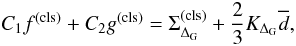 (28)the closure coefficients
are given by the linear system of equations
(28)the closure coefficients
are given by the linear system of equations ![\begin{eqnarray} \label{eq:coeff_lse_2} &\left(\int_{\mathcal{V}} |f^{(\rm cls)}|^2\dd^{3}x\right)\,C_1 + \left(\int_{\mathcal{V}} f^{(\rm cls)}g^{(\rm cls)}\dd^{3}x\right)\,C_2\\ &=\int_{\mathcal{V}} f^{(\rm cls)}\left[\Sigma_{\Delta_{\mathrm{G}}}+\frac{2}{3}K_{\Delta_{\rm G}}\overline{d}\right]\,\dd^{3}x, \\ &\left(\int_{\mathcal{V}}f^{(\rm cls)}g^{(\rm cls)} \dd^{3}x\right)\,C_1 + \left(\int_{\mathcal{V}} |g^{(\rm cls)}|^{2}\dd^{3}x\right)\,C_{2} \\ &=\int_{\mathcal{V}} g^{(\rm cls)}\left[\Sigma_{\Delta_{\mathrm{G}}}+\frac{2}{3}K_{\Delta_{\rm G}}\overline{d}\right]\,\dd^{3}x, \end{eqnarray}](/articles/aa/full_html/2011/04/aa15630-10/aa15630-10-eq140.png) where
where
 The
solutions for C1 and C2 that are
obtained from our numerical data are listed in Table 2. As one can see, the correlation coefficients are about as high as for the
purely nonlinear closure and there is only little variation with the forcing and the
filter length scale. For ΔG = 64Δ the ratio of ΔG to the integral
scale L is 8, which is quite small. As a consequence, the driving force
marginally influences this length scale. The filter length ΔG = 16Δ, on the
other hand, is significantly affected by numerical dissipation. The correlation diagrams
for the mixed closure are plotted in Fig. 4. Although
the relation between
The
solutions for C1 and C2 that are
obtained from our numerical data are listed in Table 2. As one can see, the correlation coefficients are about as high as for the
purely nonlinear closure and there is only little variation with the forcing and the
filter length scale. For ΔG = 64Δ the ratio of ΔG to the integral
scale L is 8, which is quite small. As a consequence, the driving force
marginally influences this length scale. The filter length ΔG = 16Δ, on the
other hand, is significantly affected by numerical dissipation. The correlation diagrams
for the mixed closure are plotted in Fig. 4. Although
the relation between  and Σ32Δ is slightly tilted for negative fluxes, the results are comparable to
Figs. 1d and 2d. This can also be seen in Fig. 3.
Therefore, we base our SGS model on the mixed nonlinear closure (8) with the averaged coefficients
C1 = 0.02 and C2 = 0.7.
and Σ32Δ is slightly tilted for negative fluxes, the results are comparable to
Figs. 1d and 2d. This can also be seen in Fig. 3.
Therefore, we base our SGS model on the mixed nonlinear closure (8) with the averaged coefficients
C1 = 0.02 and C2 = 0.7.
Closure and correlation coefficients for the linear combination of the eddy-viscosity and the nonlinear closure.
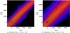 |
Fig. 4 Correlation diagrams for the mixed closures for isothermal supersonic turbulence with different forcing. |
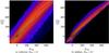 |
Fig. 5 Correlation diagrams for the mixed closure in the case of isothermal a) and adiabatic b) turbulence with lower rms Mach numbers as in Fig. 4. |
3.3. Supplementary tests for different Mach numbers
For the data listed in Table 2, the average Mach
numbers associated with the filter scale,  , assume values around the
speed of sound. Thus, the question arises whether the closure coefficients calculated
above are applicable to subsonic velocity fluctuations. To test the mixed closure for a
different Mach number, we calculated the turbulence energy flux
, assume values around the
speed of sound. Thus, the question arises whether the closure coefficients calculated
above are applicable to subsonic velocity fluctuations. To test the mixed closure for a
different Mach number, we calculated the turbulence energy flux
 with fixed values C1 = 0.02 and
C2 = 0.7 for data from a simulation of isothermal turbulence
with ℳrms ≈ 2.2 (Schmidt et al. 2009).
The resulting correlation diagram is plotted in Fig. 5a. There is a small bias to overestimate the turbulence energy flux, but the
prediction of the mixed closure is still very good. Indeed, a correlation coefficient
with fixed values C1 = 0.02 and
C2 = 0.7 for data from a simulation of isothermal turbulence
with ℳrms ≈ 2.2 (Schmidt et al. 2009).
The resulting correlation diagram is plotted in Fig. 5a. There is a small bias to overestimate the turbulence energy flux, but the
prediction of the mixed closure is still very good. Indeed, a correlation coefficient
![\hbox{$\mathrm{corr}[\Sigma_{\rm G},\Sigma_{\rm G}^{(\rm cls)}]=0.990$}](/articles/aa/full_html/2011/04/aa15630-10/aa15630-10-eq154.png) is
obtained in this case (see Table 3). In addition,
we investigated data from an adiabatic turbulence simulation (Schmidt et al. 2007), in which the rms Mach number gradually decreases
with time because of the dissipative heating of the gas. The results are summarized in
Table 3, and the correlation diagram for the
final snapshot of the simulation is shown in Fig. 5b.
Our results suggest that the closure coefficients are not very sensitive to the Mach
number. Nevertheless, we cannot exclude that the optimal values of
C1 and C2 differ significantly
if the SGS turbulence Mach number ℳsgs (see Sect. 2) is only a tiny fraction of the speed of sound. Answering this question is
left for future studies.
is
obtained in this case (see Table 3). In addition,
we investigated data from an adiabatic turbulence simulation (Schmidt et al. 2007), in which the rms Mach number gradually decreases
with time because of the dissipative heating of the gas. The results are summarized in
Table 3, and the correlation diagram for the
final snapshot of the simulation is shown in Fig. 5b.
Our results suggest that the closure coefficients are not very sensitive to the Mach
number. Nevertheless, we cannot exclude that the optimal values of
C1 and C2 differ significantly
if the SGS turbulence Mach number ℳsgs (see Sect. 2) is only a tiny fraction of the speed of sound. Answering this question is
left for future studies.
 |
Fig. 6 Visualization of the SGS turbulence energy density Ksgs in a 5123 LES with solenoidal forcing. |
3.4. Energy dissipation
For the turbulence energy on the length scale ΔG, which is defined by
Eq. (20), a dynamical equation analogous
to Eq. (7) can be formulated. By averaging
this equation over the whole periodic domain and assuming statistical equilibrium, i.e.,
∂t ⟨ KΔG ⟩ ≃ 0,
the following global balance equation is obtained:
 (35)The first term is
the mean turbulence energy flux, the second term is the mean pressure dilatation (see
Schmidt et al. 2006a), and the third term is the
mean dissipation rate expressed in terms of KΔG.
Substituting Eq. (18) for
ΣΔG yields the coefficient of turbulence energy dissipation,
Cϵ. From the supersonic isothermal
turbulence data, we find a value Cϵ ≈ 1.5,
which is somewhat higher yet still comparable to typical values calculated for
incompressible turbulence (see Sagaut 2006).
(35)The first term is
the mean turbulence energy flux, the second term is the mean pressure dilatation (see
Schmidt et al. 2006a), and the third term is the
mean dissipation rate expressed in terms of KΔG.
Substituting Eq. (18) for
ΣΔG yields the coefficient of turbulence energy dissipation,
Cϵ. From the supersonic isothermal
turbulence data, we find a value Cϵ ≈ 1.5,
which is somewhat higher yet still comparable to typical values calculated for
incompressible turbulence (see Sagaut 2006).
4. Large eddy simulations of forced supersonic turbulence
Correlation coefficients for the linear combination of the eddy-viscosity and the nonlinear closure with C1 = 0.02 and C2 = 0.7 for isothermal turbulence and adiabatic turbulence at various instants with different Mach numbers.
To investigate statistical properties of the SGS turbulence energy and related quantities, we run LES of forced supersonic isothermal turbulence with the SGS model defined in Sects. 2 and 3. For the implementation, we use the code Enzo 1.5 developed by the Laboratory for Computational Astrophysics at the University of California in San Diego (http://lca.ucsd.edu). In these simulations, we apply solenoidal, compressive and mixed force fields to produce statistically stationary and homogeneous turbulence with different rms Mach numbers (see Schmidt et al. 2006c; Schmidt et al. 2009; Federrath et al. 2010b). The forcing acts on length scales around the integral length L, where L is one half of the box size. The autocorrelation time of the force field is given by the time scale T = L/V, where the characteristic velocity V specifies the magnitude of the turbulent velocity fluctuations on the integral scale. The mixture of solenoidal (divergence-free) and compressive (rotation-free) modes of the force field is adjusted by means of a Helmholtz decomposition with weighing parameter 0 ≤ ζ ≤ 1. Purely solenoidal forcing results for ζ = 1. When setting the adiabatic exponent γ = 1.001, the energy dissipated per integral time is much lower than the internal energy for ℳrms up to about 10. For this reason, the gas is pseudo-isothermal. This approximate treatment of isothermality enables us to monitor energy conservation. With our implementation of the SGS model, the sum of resolved kinetic energy, SGS turbulence energy, and internal energy minus the power of the forcing integrated over time is conserved for the whole computational domain to a relative precision better than 10-8. The fraction of computational time consumed by the SGS model is in the percent range.
4.1. Correlations with resolved flow quantities and the effective pressure
As an example, Fig. 6 shows a visualization of
Ksgs prepared from an LES with 5123 grid cells.
The parameters of this simulation were chosen to match the ILES with solenoidal forcing in
Sect. 3.1. The rms Mach number of the flow is about
5.5 in the statistically stationary regime. In the reddish regions,
Ksgs is higher than the spatial mean, while it is lower in
the bluish regions. For comparison, Fig. 7 shows the
local denstrophy  , which is an indicator
of compressible turbulent velocity fluctuations (Kritsuk
et al. 2007). It appears that high SGS turbulence energy is concentrated in
regions of intense denstrophy. On average,
Ksgs ~ 0.1Δ2Ω1/2
for high denstrophy values, as one can see in the correlation diagram of
Ksgs vs. Δ2Ω1/2 in
Fig. 8a. The same relation is found for compressive
forcing (see panel (b) of Fig. 8). Nevertheless, the
local values of Ksgs and
Δ2Ω1/2 deviate substantially from the average
relation. This is a consequence of the various processes contributing to the SGS dynamics,
which are not fully encompassed by the derivative of the resolved velocity field. For this
reason, derived quantities such as the rate of strain or the denstrophy are only of
limited utility for estimating the effects of turbulence on unresolved length scales.
Since , this applies
also to the turbulent pressure.
, which is an indicator
of compressible turbulent velocity fluctuations (Kritsuk
et al. 2007). It appears that high SGS turbulence energy is concentrated in
regions of intense denstrophy. On average,
Ksgs ~ 0.1Δ2Ω1/2
for high denstrophy values, as one can see in the correlation diagram of
Ksgs vs. Δ2Ω1/2 in
Fig. 8a. The same relation is found for compressive
forcing (see panel (b) of Fig. 8). Nevertheless, the
local values of Ksgs and
Δ2Ω1/2 deviate substantially from the average
relation. This is a consequence of the various processes contributing to the SGS dynamics,
which are not fully encompassed by the derivative of the resolved velocity field. For this
reason, derived quantities such as the rate of strain or the denstrophy are only of
limited utility for estimating the effects of turbulence on unresolved length scales.
Since , this applies
also to the turbulent pressure.
The phase diagrams of the effective pressure (6) vs. the mass density are plotted in Fig. 9 for both LES. One can see that the average of the effective pressure for a given mass density closely follows the isothermal relation P ∝ ρ. This is because the mean turbulent pressure is small compared to the thermal pressure for the resolution Δ = L/256 (see Sect. 4.2). Locally, however, the intermittency of turbulent velocity fluctuations can give rise to an effective pressure that exceeds the thermal pressure by one order of magnitude. For this reason, the contribution of the turbulent pressure Psgs is locally not negligible. This effect becomes stronger as the cutoff scale Δ increases in comparison to the integral scale of turbulence.
In Sect. 2, we argue that the viscous stress term in
the filtered momentum Eq. (3) vanishes in
the limit of infinite Reynolds number, and the rate of energy dissipation on the grid
scale, ϵ, is determined by the SGS turbulence energy (see Eq. (10)). In contrast, an extrapolation of the
expression for the microscopic dissipation rate on length scales
ℓ ~ η to the grid scale Δ was proposed by Pan et al. (2009):  (36)The grid-scale
viscosity νΔ = const. in the above expression
is treated as a constant coefficient that is determined by the mean numerical dissipation
of PPM. Defining the compressible Reynolds number of the resolved flow by
(36)The grid-scale
viscosity νΔ = const. in the above expression
is treated as a constant coefficient that is determined by the mean numerical dissipation
of PPM. Defining the compressible Reynolds number of the resolved flow by
 , where
urms is the root mean square velocity5, the viscosity can be evaluated from
νΔ = VL/ReΔ.
The problem with this approach is that the viscosity on the grid scale, which corresponds
to the SGS eddy-viscosity, cannot be assumed to be constant.
, where
urms is the root mean square velocity5, the viscosity can be evaluated from
νΔ = VL/ReΔ.
The problem with this approach is that the viscosity on the grid scale, which corresponds
to the SGS eddy-viscosity, cannot be assumed to be constant.
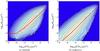 |
Fig. 8 Correlation diagrams of the SGS turbulence energy vs. the denstrophy, normalized by the cutoff scale Δ, for 5123 LES with solenoidal and compressive forcing. The contours are logarithmic. The average relation between both quantities is indicated by the dotted lines, and the dashed line shows the relation Ksgs ~ 0.1Δ2Ω1/2. |
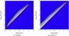 |
Fig. 9 Phase diagrams of the effective pressure defined by Eq. (6) vs. the mass density for 5123 LES with solenoidal and compressive forcing. The contours are logarithmic. The averages of the SGS turbulence energy for particular values of the denstrophy are indicated by the dotted lines. |
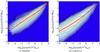 |
Fig. 10 Correlation diagrams of the normalized rate of energy dissipation defined by Eq. (36), where νΔ assumes a constant value that is given by the numerical Reynolds number, vs. the rate of energy dissipation (10) that is predicted by the SGS model. The averages of expression (36) for given values of ϱϵsgs are indicated by the dotted lines. |
When neglecting diffusion, compressibility, and the nonlinear term in the SGS turbulence stress (8), the equilibrium between production and dissipation of SGS turbulence energy in Eq. (7) implies Ksgs ~ (C1/Cϵ)ϱΔ2|S∗|2, hence, ϵ ~ (Δ/Cϵ)2(C1|S∗|)3 according to Eq. (10). We emphasize that a relation of the form ϵ ~ Δ2|S∗|3 follows from any common SGS model under the assumption of local equilibrium (Sagaut 2006). Comparing to Eq. (36), we see that that νΔ ~ Δ2|S∗|, which is not a constant. This is because ϱϵ ≠ σijui,j ∝ |S∗|2, as explained in Sect. 2. The discrepancy becomes apparent in Fig. 10, which shows the correlation diagrams of the rate of energy dissipation calculated via Eq. (36) vs. ϵ following from the SGS model. Toward low values of ϵ, we find an average relation close to |S∗|2 ∝ ϵ2/3, which is just the relation that follows from the above estimate of the equilibrium dissipation rate. This behaviour is reasonable because the contribution of the nonlinear term in the closure (8), which is neglected in the estimate, is relatively small for low values of Ksgs (corresponding to low energy dissipation). Moreover, the unresolved velocity fluctuations tend to be significantly smaller than the speed of sound in this limit, which corresponds to low compressibility. Consequently, the results from the LES support the theoretical arguments against Eq. (36) as an approximation to the dissipation rate on the grid scale. Although Eqs. (10) and (36) yield about the same mean dissipation rate, the former determines the local rate of energy dissipation on the footing of a physically well motivated scale-separation of fluid dynamics, while the latter is based on a putative analogy between the numerical and the microscopic viscosity.
4.2. Dependence on the cutoff scale
Time-averaged spatial mean values of various quantities and their standard deviations from the averages for different numerical resolutions.
The scaling of the turbulent velocity fluctuations in supersonic hydrodynamic turbulence has been inferred from energy spectrum functions and structure functions (e.g., Kritsuk et al. 2007; Schmidt et al. 2008, 2009; Federrath et al. 2010b; Price & Federrath 2010). The pure velocity scaling in the supersonic regime is stiffer than Kolmogorov scaling, and it appears that the scaling exponent depends on the forcing. For example, Federrath et al. (2010b) find indices of the turbulence energy spectra β = −1.86 ± 0.05 and −1.94 ± 0.05 for solenoidal and compressive forcing, respectively. For incompressible turbulence, β = −5/3. Velocity variables with fractional massweighing, in particular ρ1/3u, exhibit similar scaling laws, which can be interpreted as indicating universality (Kritsuk et al. 2007; Schmidt et al. 2008).
The SGS turbulence energy is given by the fluctuations in the velocity and density fields
on length scales ℓ ≲ Δ, as defined by Eqs. (4) and (5). However,
there is no obvious relation to the known scaling laws for turbulence, because the
decomposition of the fluid dynamical variables cannot be related to the two-point
statistics (structure functions) or the Fourier modes (energy spectra) in a
straightforward manner. To determine the scaling of SGS turbulence as a function of Δ, we
run several LES with Δ ranging from L/256 to
L/32. The mean values of the rms Mach number and the
SGS turbulence Mach number are plotted as functions of time in Fig. 11. The flow approaches a statistically stationary state after about 2
integral time scales (Schmidt et al. 2009; Federrath et al. 2010b), for which ℳrms
settles at values between 5 and 6. The temporal variation in ℳrms is caused by
the stochastic forcing. As expected,  decreases with the cutoff scale. Averaging the spatial means from
t = 2T to 10T, we find the
time-averaged mean values listed in Table 4. As one
can see in Fig. 12a, the time averages of
closely follow power laws,
decreases with the cutoff scale. Averaging the spatial means from
t = 2T to 10T, we find the
time-averaged mean values listed in Table 4. As one
can see in Fig. 12a, the time averages of
closely follow power laws,  (37)with
αℳ = 0.475 ± 0.004 for solenoidal and 0.451 ± 0.026 for
compressive forcing.
(37)with
αℳ = 0.475 ± 0.004 for solenoidal and 0.451 ± 0.026 for
compressive forcing.
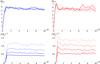 |
Fig. 11 Temporal evolution of the rms Mach number (top) and the mean SGS turbulence Mach number (bottom) for solenoidal (left column) and compressive forcing (right column). The cutoff length Δ decreases from L/32 (light colour) to L/256 (full colour). |
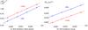 |
Fig. 12 Scaling laws for the mean SGS turbulence Mach number a) and energy b) as functions of the numerical resolution Δ. |
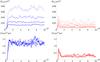 |
Fig. 13 Temporal evolution of the SGS turbulence energy (top) and the dissipation rate (bottom) for solenoidal (left column) and compressive forcing (right column). The cutoff length Δ decreases from L/32 (light colour) to L/256 (full colour). |
The behaviour of the mean SGS turbulence energy is similar, although the intermittent
fluctuations of ⟨ Ksgs ⟩ are more pronounced than the mean
SGS turbulence Mach number (see top panels of Fig. 13). The higher degree of intermittency stems from the mass density that is
included in Ksgs. For compressive forcing,
⟨ Ksgs ⟩ is systematically lower in comparison to the LES
with solenoidal forcing. This indicates that the total amount of energy in the turbulent
structures on a given length scale is smaller in the compressive forcing case. The ratio
of the mean values of Ksgs for compressive and solenoidal
forcing in Table 4 approximately agrees with the
ratio 0.38 that is inferred from the filtered high-resolution data. On the other hand, the
scaling laws 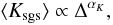 (38)are nearly the same for
solenodial and compressive forcing (see Fig. 12b).
We find the slopes αK = 0.799 ± 0.009 and
0.769 ± 0.029, which agree within the error bars. This result is remarkable, because it
suggests that the scaling properties of turbulence on small length scales are independent
of the forcing.
(38)are nearly the same for
solenodial and compressive forcing (see Fig. 12b).
We find the slopes αK = 0.799 ± 0.009 and
0.769 ± 0.029, which agree within the error bars. This result is remarkable, because it
suggests that the scaling properties of turbulence on small length scales are independent
of the forcing.
As can be seen in the bottom panels of Fig. 13, the above scaling law of ⟨ Ksgs ⟩ results in a mean dissipation rate ⟨ ρϵ ⟩ that is independent of the cutoff scale, which is an essential property of the energy dissipation predicted by the SGS model. The time-averaged mean values are listed in Table 4. Since turbulence is statistically stationary in these simulations, the constant rate of energy dissipation corresponds to a mean turbulence energy flux that is also constant. Theoretical arguments implying the existence of a scale-free energy flux in the compressible turbulent cascade have recently been presented by Aluie (2011). The significantly lower mean dissipation rate in the case of compressive forcing is consistent with the energy spectra of ρ1/3u (see Fig. A.1, in Federrath et al. 2010b). This mass-weighted velocity variable is related to the energy dissipation rate (Kritsuk et al. 2007). Moreover, Fig. 14 (left panel) shows that the growth of the mean internal energy in time becomes smaller as the weighing parameter ζ decreases from 1 (solenodial forcing) to 0 (compressive forcing). After subtracting the contribution from numerically resolved compression effects (see Schmidt et al. 2006c), we find that, independent of the cutoff length Δ, about 3/4 of the change of the internal energy stems from SGS turbulence energy dissipation. The remainder is caused by numerical dissipation. This does not imply that the total rate of energy dissipation is much higher in LES than in ILES, because the total energy dissipation is always determined by the energy injection due to the forcing. In conclusion, the greater part of kinetic energy is dissipated through the SGS turbulence energy reservoir at a scale-free rate.
To quantify the relative importance of high values of ℳsgs, we determined the volume fractions of cells with an SGS turbulence Mach number greater than a particular value. This fraction is given by 1 − cdf(ℳsgs), where cdf(ℳsgs) is the cumulative distribution function of ℳsgs. In Fig. 15, the resulting functions are plotted for the LES with different cutoff lengths. As expected, the fraction with ℳsgs > 1 decreases with the cutoff length Δ. However, the tails toward high ℳsgs demonstrate that even at relatively high resolution there are supersonic velocity fluctuations on unresolved length scales, and the corresponding turbulent pressure decreases only a little with the cutoff scale.
 |
Fig. 14 Left panel: time evolution of the mean internal energy for forcing with varying ζ and about the same rms Mach number. Right panel: volume fractions of zones, in which the SGS turbulence Mach number is greater than any given value for the same forcing parameters as in the left panel (the curves for ζ = 1 and ζ = 2/3 almost coincide). |
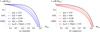 |
Fig. 15 Volume fractions of zones, in which the SGS turbulence Mach number is greater than a certain value for different numerical resolutions. The dashed lines follows from the filtering of 10243 ILES data with filter length 16Δ. This corresponds to the 643 LES, for which Δ/L = 1/32. |
For the lowest resolution LES, we can compare the distribution of ℳsgs to the distribution inferred from the corresponding filtered 10243 data (see Sect. 3.1). The filter length ΔG = 16Δ = L/32 is equivalent to the cutoff length in the 643 LES. Choosing an even lower resolution of the LES, corresponding to a larger filter length for the ILES, turned out not to be feasible. Even for the LES with Δ/L = 1/32, the forcing range and the range of length scales that are directly affected by numerical dissipation overlap. For the filtering of the ILES, on the other hand, the filter length cannot be lowered (corresponding to a higher resolution of the LES), because the dynamical range of fluctuations between the grid scale and the filter length would become insufficient and the numerical smoothing would be too strong. Nevertheless, Fig. 15a demonstrates that the distributions agree remarkably well in the case of solenoidal forcing. For compressive forcing, there are larger discrepancies. However, given that Gaussian filtering only corresponds roughly to the implicit filter in an LES and that the SGS model is based on various approximations, the match is quite satisfactory.
The larger deviations in the case of compressive forcing suggest that it is not possible to calibrate the SGS model coefficients in such a way that an optimal match is obtained both for solenoidal and for compressive forcing at the same time. The different shape of the distribution that is obtained from the high-resolution simulation with compressive forcing points toward a missing physical effect such as the pressure-dilatation, which is entirely neglected in our SGS model. Either way, purely compressive forcing is a limiting case. In nature, some mixture of solenoidal and compressive forcing is more likely to occur. In Fig. 14 (right panel), we compare the distributions of ℳsgs for force fields with ζ varying from 1 (solenoidal) to 0 (compressive). High SGS turbulence Mach numbers become more frequent as the contribution of compressive forcing modes increases.
Time-averaged spatial mean values of various quantities and their standard deviations from the averages for different forcing magnitudes (defined by Ma = V/c0) and mixtures of solenoidal and compressive modes.
4.3. Dependence on the Mach number
At fixed resolution, the SGS turbulence energy increases with the resolved kinetic energy of the flow. For isothermal turbulence, this also implies an increase in the SGS turbulence Mach number with rising rms Mach number. To investigate this dependence, we varied the magnitude of mixed forcing with ζ = 2/3 and ζ = 1/3. In the case ζ = 1/2, a forcing field with two solenoidal and one longitudinal degrees of freedom is obtained. Figure 8 in Federrath et al. (2010b) demonstrates that the ratio of the energy that is contained in transversal and longitudinal modes approaches a constant value for ζ > 1/2 (see also Kritsuk et al. 2010). Correspondingly, the cumulative distributions of ℳsgs plotted in Fig. 14b show that there is almost no difference between forcing with ζ = 2/3 and purely solenoidal forcing (ζ = 1). On the other hand, one can see that there is a noticeable influence of compressive modes for ζ = 1/3, but the distribution differs from the purely compressive case (ζ = 0).
The dependence of the RMS SGS turbulence Mach number on the forcing amplitude is shown in
the top panels of Fig. 16 for 2563 LES.
The corresponding characteristic Mach numbers and time-averaged statistics are listed in
Table 5. Independent of the Mach number, the
ratio of to
ℳrms is nearly equal for ζ = 2/3 and
1/3. This ratio is 0.102 for purely solenoidal forcing
(ζ = 1), and 0.138 for purely compressive forcing
(ζ = 0). Consequently,  is mostly determined
by the grid scale Δ, except for small ζ. As one can see in the middle
panels of Fig. 16, the normalized mean SGS
turbulence energy,
⟨ Ksgs ⟩ /ρ0V2,
is about the same for the different Mach numbers, with a weak trend to decrease toward low
Mach numbers (see also Table 5). The same behaviour
is found for the mean dissipation rate (Fig. 16,
bottom panels), which further supports the validity of the SGS model in the supersonic
regime. Following the trend discussed in Sect 4.2,
clearly the mixture of solenoidal and compressive forcing modes has an influence.
is mostly determined
by the grid scale Δ, except for small ζ. As one can see in the middle
panels of Fig. 16, the normalized mean SGS
turbulence energy,
⟨ Ksgs ⟩ /ρ0V2,
is about the same for the different Mach numbers, with a weak trend to decrease toward low
Mach numbers (see also Table 5). The same behaviour
is found for the mean dissipation rate (Fig. 16,
bottom panels), which further supports the validity of the SGS model in the supersonic
regime. Following the trend discussed in Sect 4.2,
clearly the mixture of solenoidal and compressive forcing modes has an influence.
Figure 17 shows the distributions of ℳsgs for ζ = 2/3 (a) and 1/3 (b), as explained in Sect. 4.2. For both forcing types, the volume fractions with ℳsgs > 1 increase with the forcing magnitude. For rms Mach numbers greater than 5, supersonic turbulent velocity fluctuations at the cutoff scale fill more then 10% of the total volume. If the ratio between the integral scale of turbulence and the cutoff scale is less, the volume filling factor increases further.
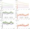 |
Fig. 16 Temporal evolution of the SGS turbulence Mach number (top) and energy (middle) and the dissipation rate (bottom) for ζ = 2/3 (left column) and ζ = 1/3 (right column). The different lines in each plot correspond to different forcing magnitudes (see Table 5), which are specified by the values of the characteristic Mach number Ma = V/c0 (c0 is the initial speed of sound). |
5. Conclusion
In formulating a mixed closure for the flux of energy from the numerically resolved to the unresolved scales, we generalized the subgrid-scale (SGS) turbulence energy model to the regime of highly compressible turbulence. This closure is based on ideas of Woodward et al. (2006) and features a nonlinear term in addition to a linear eddy-viscosity term. In general, the turbulence energy cascade is an important source of SGS turbulence energy production in turbulent flows, and it should not be neglected even if other subresolution sources are emphasized in particular astrophysical applications (e.g., Scannapieco & Brüggen 2008; Joung et al. 2009). Our proposed closure for the transfer of energy by the turbulent cascade complements theses models. We verified this closure by means of explicit filtering of high-resolution data from various simulations of supersonic isothermal and adiabatic turbulence (Schmidt et al. 2007, 2009; Federrath et al. 2010b). Tests in large eddy simulations of forced supersonic turbulence show that the SGS model meets several important requirements that should be satisfied by any sound SGS model:
-
for statistically stationary turbulence, an equilibrium betweenthe production and the dissipation of SGS turbulence is reached.The mean SGS turbulence energy depends on the grid scale via apower law;
-
the SGS turbulence Mach number, which specifies the importance of the turbulent pressure on the grid scale relative to the thermal pressure of the gas, depends linearly on the rms Mach number of the resolved turbulence;
-
the SGS turbulence energy dissipation is independent of the grid scale.
Forced turbulence simulations in a periodic box are very suitable to testing the properties listed above, because of the well-defined statistics of the isotropic, homogeneous and stationary turbulence that is produced. In addition to these properties, we find a dependence of the SGS turbulence energy and the rate of energy dissipation on the mixture of solenoidal (divergence-free) and compressive (rotation-free) forcing modes. However, the scaling laws for the SGS turbulence energy are very similar for solenoidal and compressive forcing. This indicates that the SGS model describes the dynamics in the inertial subrange, although the length scales close to the cutoff scale are affected by numerical dissipation. The differences in the mean values result from the substantial differences in the turbulent flow structure on larger scales (see Federrath et al. 2008, 2009, 2010b).
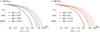 |
Fig. 17 Volume fractions of zones, in which the SGS turbulence Mach number is greater than any given value for different rms Mach numbers and mixtures of solenoidal and compressive modes, as in Fig. 16. |
The implementation of the SGS model into a fluid-dynamical code such as Enzo is rather straightforward. The SGS turbulence energy can be treated as a passive scalar with various source terms. To evaluate the mixed closure for the turbulence energy cascade, derivatives of the resolved velocity field are computed by means of centred differences. Care must be taken to ensure energy conservation, particularly if the net change of the SGS turbulence energy in a certain grid cell exhausts the available energy over a time step or, vice-versa, if too much energy is drained from the resolved scales. However, these are exceptions that can be handled numerically. The effective increase in computing time is less than 10%. Moreover, the hydrodynamic coupling of the SGS model to the resolved flow introduces a reduction of the bottleneck effect in the turbulence energy spectra (Woodward et al. 2006; Schmidt 2010).
In our large eddy simulations, we find correlations between resolved flow quantities, such as the rate of strain or the denstrophy and SGS quantities, but the scatter is large. This is problematic if one intends to estimate unresolved flow properties on the basis of such correlations. In particular, this applies to the calculation of the dissipation rate from a constant numerical viscosity and the rate of strain, as proposed by Pan et al. (2009). We have shown that the assumption of a constant numerical dissipation coefficient is inconsistent with the equilibrium relation between the dissipation rate and the rate of strain on the grid scale in the limit of large Reynolds numbers. This relation, which follows from the SGS turbulence energy model with the linear eddy-viscosity closure (and also from the Smagorinsky model), is verified by our LES data for low turbulence intensity, while deviations become apparent for strong turbulent dissipation. This can be understood as a consequence of the nonlinear term in the closure for the turbulence energy flux. Also the estimate of turbulent pressure effects using the rate of strain and the vorticity of the resolved flow that is put forward by Zhu et al. (2010) is incomplete because they do not distinguish between the contributions from the resolved flow and from the subgrid scales. The predictions from both approaches with regard to turbulence in the intergalactic medium are compared in ongoing work (Iapichino et al. 2011).
From the probability distributions of the SGS turbulence Mach number, it follows that the turbulent pressure locally exceeds the thermal pressure even at moderate rms Mach numbers and for relatively small grid scales. Since the grid scale in contemporary galactic disk simulations (e.g., Agertz et al. 2009; Tasker & Tan 2009) is close to molecular cloud scales (a few pc), unresolved supersonic velocity fluctuations are quite likely and the turbulent pressure plays an important role. This has implications for the treatment of collapsing gas regions. The criterion for gravitational stability, which influences the grid resolution in adaptive mesh refinement simulations and controls the production of sink particles to capture the collapsing gas, is usually based on the thermal Jeans mass (among other criteria; see Federrath et al. 2010a). To account for the effects of turbulence below the grid scale, we suggest including the turbulent pressure in the definition of the Jeans mass, in analogy to the magnetic pressure in self-gravitating MHD turbulence.
To model the fragmentation below the grid scale in more detail, a possible approach could be based on the assumption that the local star formation efficiency is regulated by turbulence on the grid scale. Then the star formation rate can be parameterized in terms of the turbulent Mach number that is calculated from the SGS model (see Krumholz & McKee 2005; Padoan & Nordlund 2009). On the other hand, star formation acts back on the SGS turbulence energy via stellar feedback. As suggested by Joung et al. (2009), a stellar feedback term can be included in the SGS turbulence energy equation. Statistically, we have
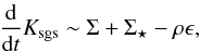 where
Σ⋆ ∝ ρe ⋆ /τff
accounts for the energy injection per unit mass,
e⋆, by supernovae. The associated time
scale is the free-fall time scale
τff = [3π/(32Gρ)] 1/2,
which is the fundamental time scale of star formation. Neglecting the fluctuations of the
gas density and setting the mean production rate
Σ ~ V2/T, where
V and T are the typical velocity and the turn-over time
scale, respectively, of the resolved turbulent flow, it follows that the turbulent pressure
in equilibrium is of the order
where
Σ⋆ ∝ ρe ⋆ /τff
accounts for the energy injection per unit mass,
e⋆, by supernovae. The associated time
scale is the free-fall time scale
τff = [3π/(32Gρ)] 1/2,
which is the fundamental time scale of star formation. Neglecting the fluctuations of the
gas density and setting the mean production rate
Σ ~ V2/T, where
V and T are the typical velocity and the turn-over time
scale, respectively, of the resolved turbulent flow, it follows that the turbulent pressure
in equilibrium is of the order ![\begin{equation} \label{eq:energy_eq_fb} P_{\rm sgs} \sim \rho\Delta^{2/3} \left[\frac{V^{2}}{T} + C_{\star}\frac{e_{\star}}{\tau_{\rm ff}}\right]^{2/3}\cdot \end{equation}](/articles/aa/full_html/2011/04/aa15630-10/aa15630-10-eq293.png) (39)Kolmogorov scaling becomes
manifest in the factor Δ2/3 in Eq. (39). For highly compressible turbulence,
however, the scaling of the SGS turbulence energy deviates from the Kolmogorov law (see
Sect. 4.2). Depending on the ratios
V2/e ⋆
and T/τff, the production of
SGS turbulence energy by the turbulent cascade or by supernovae dominates. The model of
Joung et al. (2009) follows in the limit
(V2/e ⋆ )(τff/T) ≪ 1.
In general, shear instabilities, gravitational instabilities, cooling instabilities, etc.
above the grid scale feed energy to smaller scales. For disk galaxies, a simple estimate can
be obtained from the velocity dispersion of atomic hydrogen, which is about
10 km s-1. Agertz et al. (2009) show
that gravitational instabilities grow on length scales ranging from 0.1 to about 2 kpc.
Setting V = 106 cm s-1 and assuming
L > 0.1 kpc ≈ 3 × 1020 cm, the
turbulence energy flux to smaller length scales is
V2/T = V3/L ≲ 0.003 erg g-1 s-1.
On the other hand,
(39)Kolmogorov scaling becomes
manifest in the factor Δ2/3 in Eq. (39). For highly compressible turbulence,
however, the scaling of the SGS turbulence energy deviates from the Kolmogorov law (see
Sect. 4.2). Depending on the ratios
V2/e ⋆
and T/τff, the production of
SGS turbulence energy by the turbulent cascade or by supernovae dominates. The model of
Joung et al. (2009) follows in the limit
(V2/e ⋆ )(τff/T) ≪ 1.
In general, shear instabilities, gravitational instabilities, cooling instabilities, etc.
above the grid scale feed energy to smaller scales. For disk galaxies, a simple estimate can
be obtained from the velocity dispersion of atomic hydrogen, which is about
10 km s-1. Agertz et al. (2009) show
that gravitational instabilities grow on length scales ranging from 0.1 to about 2 kpc.
Setting V = 106 cm s-1 and assuming
L > 0.1 kpc ≈ 3 × 1020 cm, the
turbulence energy flux to smaller length scales is
V2/T = V3/L ≲ 0.003 erg g-1 s-1.
On the other hand,  and C ⋆ ≈ 0.025 imply
Σ ⋆ ~ 0.03η (n/1 cm-3)1/2 erg g-1 s-1
(see Joung et al. 2009). Since the efficiency of the
energy transfer from supernova blast waves to the interstellar gas is roughly
η ≃ 0.1 (Mac Low & Klessen
2004), the energy injection by stellar feedback is comparable to the turbulence
energy flux for atomic hydrogen with density n ~ 1 cm-3. The
dependence of Σ ⋆ on the gas density implies a greater
contribution from supernova feedback in the cold-gas phase, but the above estimate does not
account for the intermittency of turbulent velocity fluctuations, which entails large
deviations from the mean. As a consequence, the assumption of Joung et al. (2009) to consider the energy injection by supernova as the
main source of the turbulent pressure is marginally fulfiled in cosmological simulations, in
which the internal structure of galaxies is very poorly resolved. In galactic-scale
simulations with high resolution, on the other hand, turbulence is not uniformly produced,
and including the turbulence energy cascade improves the description of numerically
unresolved processes. In particular, it will be useful to attempt a further generalization
of the SGS model to multiphase turbulence. A very simple ansatz has recently been presented
by Murante et al. (2010). A complete SGS model that
treats a warm and a cold gas phase is presently under development (Braun & Schmidt,
in prep.).
and C ⋆ ≈ 0.025 imply
Σ ⋆ ~ 0.03η (n/1 cm-3)1/2 erg g-1 s-1
(see Joung et al. 2009). Since the efficiency of the
energy transfer from supernova blast waves to the interstellar gas is roughly
η ≃ 0.1 (Mac Low & Klessen
2004), the energy injection by stellar feedback is comparable to the turbulence
energy flux for atomic hydrogen with density n ~ 1 cm-3. The
dependence of Σ ⋆ on the gas density implies a greater
contribution from supernova feedback in the cold-gas phase, but the above estimate does not
account for the intermittency of turbulent velocity fluctuations, which entails large
deviations from the mean. As a consequence, the assumption of Joung et al. (2009) to consider the energy injection by supernova as the
main source of the turbulent pressure is marginally fulfiled in cosmological simulations, in
which the internal structure of galaxies is very poorly resolved. In galactic-scale
simulations with high resolution, on the other hand, turbulence is not uniformly produced,
and including the turbulence energy cascade improves the description of numerically
unresolved processes. In particular, it will be useful to attempt a further generalization
of the SGS model to multiphase turbulence. A very simple ansatz has recently been presented
by Murante et al. (2010). A complete SGS model that
treats a warm and a cold gas phase is presently under development (Braun & Schmidt,
in prep.).
Including stellar feedback and cooling into our SGS model will be of further utility for the numerical treatment of turbulence in the intergalactic medium (see Springel & Hernquist 2003), where turbulence is produced by different processes (see, for instance, Cen & Ostriker 1999; Subramanian et al. 2006; Ryu et al. 2008; Iapichino et al. 2008, 2011). Oppenheimer & Davé (2009) show that a significant amount of the line broadening of O VI in cosmological simulations stems from numerically unresolved turbulence. They apply a heuristic model in the postprocessing of the simulation data. When using an SGS model, on the other hand, the effect on the line broadening can be computed on the fly. Moreover, metals are mixed into the intergalactic medium by turbulence that is driven by galactic outflows. SGS turbulence enhances the turbulent mixing. Following an approach that is quite similar to the treatment of stellar feedback in galaxy simulations, our SGS model can be used in combination with phenomenological models for supernova-driven outflows (Joung et al. 2009; Evoli & Ferrara 2011). In both cases, the use of adaptive mesh refinement is mandatory for achieving a sufficient dynamical range. Therefore, an essential objective for future work will be to incorporate the new closure for the highly compressible turbulent cascade into fluid mechanics with adaptively refined large eddy simulations (FEARLESS; Maier et al. 2009).
The eddy-viscosity closure depends on  .
Writing
.
Writing  , a factor
qsgs can be cancelled from the SGS turbulence energy
Eq. (7). This results in an equation for
qsgs with a nonvanishing production rate of
qsgs even starting from the initial condition
qsgs = 0. For the nonlinear closure, on the other hand,
qsgs = 0 is a fixed point of the equation.
, a factor
qsgs can be cancelled from the SGS turbulence energy
Eq. (7). This results in an equation for
qsgs with a nonvanishing production rate of
qsgs even starting from the initial condition
qsgs = 0. For the nonlinear closure, on the other hand,
qsgs = 0 is a fixed point of the equation.
See Schmidt et al. (2009). Here, we replace
 by
by
 for
consistency with Eq. (36).
for
consistency with Eq. (36).
Acknowledgments
We thank Jens Niemeyer and Ralf Klessen for valuable discussions. Computations described in this work were performed using the Enzo code developed by the Laboratory for Computational Astrophysics at the University of California in San Diego (http://lca.ucsd.edu). The computational resources were provided by the HLRBII project h0972 at the Leibniz Supercomputer Centre in Garching, Germany. C.F. acknowledges funding from the Landesstiftung Baden-Würrtemberg via their programme International Collaboration II (grant P-LS-SPII/18), from the German Bundesministerium für Bildung und Forschung via the ASTRONET project STAR FORMAT (grant 05A09VHA), from the International Max Planck Research School for Astronomy and Cosmic Physics (imprs-a) and from the Heidelberg Graduate School of Fundamental Physics (hgsfp), which is funded by the Excellence Initiative of the Deutsche Forschungsgemeinschaft (dfg) gsc 129/1. Furthermore, C.F. received funding from the European Research Council under the European Community’s Seventh Framework Programme (FP7/2007-2013 Grant Agreement no. 247060) for the research presented in this work.
References
- Agertz, O., Lake, G., Teyssier, R., et al. 2009, MNRAS, 392, 294 [NASA ADS] [CrossRef] [Google Scholar]
- Agertz, O., Teyssier, R., & Moore, B. 2010, MNRAS, 1527 [Google Scholar]
- Aluie, H. 2011, Phys. Rev. Lett., submitted [arXiv:1101.0455] [Google Scholar]
- Benzi, R., Biferale, L., Fisher, R. T., et al. 2008, Phys. Rev. Lett., 100, 234503 [NASA ADS] [CrossRef] [PubMed] [Google Scholar]
- Bonazzola, S., Heyvaerts, J., Falgarone, E., Perault, M., & Puget, J. L. 1987, A&A, 172, 293 [NASA ADS] [Google Scholar]
- Bonazzola, S., Perault, M., Puget, J. L., et al. 1992, J. Fluid Mech., 245, 1 [Google Scholar]
- Burkert, A., Genzel, R., Bouché, N., et al. 2010, ApJ, 725, 2324 [NASA ADS] [CrossRef] [Google Scholar]
- Cen, R., & Ostriker, J. P. 1999, ApJ, 514, 1 [NASA ADS] [CrossRef] [Google Scholar]
- Chandrasekhar, S. 1951, Roy. Soc. Lond. Proc. Ser. A, 210, 26 [Google Scholar]
- Colella, P., & Woodward, P. R. 1984, J. Comp. Physics, 54, 174 [Google Scholar]
- Dobbs, C. L., Glover, S. C. O., Clark, P. C., & Klessen, R. S. 2008, MNRAS, 389, 1097 [NASA ADS] [CrossRef] [MathSciNet] [Google Scholar]
- Evoli, C., & Ferrara, A. 2011, MNRAS, accepted [arXiv:1101.2449] [Google Scholar]
- Federrath, C., Klessen, R. S., & Schmidt, W. 2008, ApJ, 688, L79 [NASA ADS] [CrossRef] [Google Scholar]
- Federrath, C., Klessen, R. S., & Schmidt, W. 2009, ApJ, 692, 364 [NASA ADS] [CrossRef] [Google Scholar]
- Federrath, C., Banerjee, R., Clark, P. C., & Klessen, R. S. 2010a, ApJ, 713, 269 [NASA ADS] [CrossRef] [Google Scholar]
- Federrath, C., Roman-Duval, J., Klessen, R. S., Schmidt, W., & Mac Low, M. 2010b, A&A, 512, A81 [NASA ADS] [CrossRef] [EDP Sciences] [Google Scholar]
- Frisch, U. 1995, Turbulence (Cambridge University Press) [Google Scholar]
- Fureby, C., Tabor, G., Weller, H. G., & Gosman, A. D. 1997, Phys. Fluids, 9, 3578 [NASA ADS] [CrossRef] [Google Scholar]
- Germano, M. 1992, J. Fluid Mech., 238, 325 [NASA ADS] [CrossRef] [Google Scholar]
- Iapichino, L., Adamek, J., Schmidt, W., & Niemeyer, J. C. 2008, MNRAS, 388, 1079 [NASA ADS] [CrossRef] [Google Scholar]
- Iapichino, L., Schmidt, W., Niemeyer, J. C., & Merklein, J. 2011, MNRAS, submitted [Google Scholar]
- Ishihara, T., Gotoh, T., & Kaneda, Y. 2009, Ann. Rev. Fluid Mech., 41, 165 [Google Scholar]
- Joung, M. K. R., & Mac Low, M. 2006, ApJ, 653, 1266 [NASA ADS] [CrossRef] [Google Scholar]
- Joung, M. R., Mac Low, M.-M., & Bryan, G. L. 2009, ApJ, 704, 137 [NASA ADS] [CrossRef] [Google Scholar]
- Kritsuk, A. G., Norman, M. L., Padoan, P., & Wagner, R. 2007, ApJ, 665, 416 [NASA ADS] [CrossRef] [Google Scholar]
- Kritsuk, A. G., Ustyugov, S. D., Norman, M. L., & Padoan, P. 2010, in Numerical modeling of space plasma fows, ASTRONUM 2009, ed. N. V. Pogorelov, E. Audit & G. P. Zink, ASP Conf. Ser., 429, 15 [Google Scholar]
- Krumholz, M. R., & McKee, C. F. 2005, ApJ, 630, 250 [NASA ADS] [CrossRef] [Google Scholar]
- Mac Low, M.-M., & Klessen, R. S. 2004, Rev. Modern Phys., 76, 125 [Google Scholar]
- Maier, A., Iapichino, L., Schmidt, W., & Niemeyer, J. C. 2009, ApJ, 707, 40 [NASA ADS] [CrossRef] [Google Scholar]
- Murante, G., Monaco, P., Giovalli, M., Borgani, S., & Diaferio, A. 2010, MNRAS, 405, 1491 [NASA ADS] [Google Scholar]
- Oppenheimer, B. D., & Davé, R. 2009, MNRAS, 395, 1875 [NASA ADS] [CrossRef] [Google Scholar]
- Padoan, P., & Nordlund, A. 2009, ApJ, submitted [arXiv:0907.0248] [Google Scholar]
- Pan, L., Padoan, P., & Kritsuk, A. G. 2009, Phys. Rev. Lett., 102, 034501 [NASA ADS] [CrossRef] [PubMed] [Google Scholar]
- Price, D. J., & Federrath, C. 2010, MNRAS, 406, 1659 [NASA ADS] [Google Scholar]
- Röpke, F. K., & Schmidt, W. 2009, in Interdisciplinary Aspects of Turbulence, ed. W. Hillebrandt, & F. Kupka, Lecture Notes in Physics, 756, 255 [Google Scholar]
- Ryu, D., Kang, H., Cho, J., & Das, S. 2008, Science, 320, 909 [NASA ADS] [CrossRef] [PubMed] [Google Scholar]
- Sagaut, P. 2006, Large eddy simulation for incompressible flows: An introduction (Berlin: Springer-Verlag) [Google Scholar]
- Sarkar, S. 1992, Phys. Fluids, 4, 2674 [Google Scholar]
- Scannapieco, E., & Brüggen, M. 2008, ApJ, 686, 927 [NASA ADS] [CrossRef] [Google Scholar]
- Schmidt, W. 2010, in Numerical modeling of space plasma fows, ASTRONUM 2009, ed. N. V. Pogorelov, E. Audit & G. P. Zink, ASP Conf. Ser., 429, 45 [Google Scholar]
- Schmidt, W., Niemeyer, J. C., & Hillebrandt, W. 2006a, A&A, 450, 265 [NASA ADS] [CrossRef] [EDP Sciences] [Google Scholar]
- Schmidt, W., Niemeyer, J. C., Hillebrandt, W., & Röpke, F. K. 2006b, A&A, 450, 283 [NASA ADS] [CrossRef] [EDP Sciences] [Google Scholar]
- Schmidt, W., Hillebrandt, W., & Niemeyer, J. C. 2006c, Comp. Fluids., 35, 353 [Google Scholar]
- Schmidt, W., Niemeyer, J. C., Hupp, M., Federrath, C., & Maier, A. 2007, A New Modelling Approach for Turbulent Astrophysical Flows, DECI project report, available from URL http://www.deisa.eu/science/deci/projects2005-2006/files/fearless_report.pdf [Google Scholar]
- Schmidt, W., Federrath, C., & Klessen, R. 2008, Phys. Rev. Lett., 101, 194505 [NASA ADS] [CrossRef] [PubMed] [Google Scholar]
- Schmidt, W., Federrath, C., Hupp, M., Kern, S., & Niemeyer, J. C. 2009, A&A, 494, 127 [NASA ADS] [CrossRef] [EDP Sciences] [Google Scholar]
- Springel, V., & Hernquist, L. 2003, MNRAS, 339, 289 [Google Scholar]
- Subramanian, K., Shukurov, A., & Haugen, N. E. L. 2006, MNRAS, 366, 1437 [NASA ADS] [CrossRef] [Google Scholar]
- Tasker, E. J., & Tan, J. C. 2009, ApJ, 700, 358 [NASA ADS] [CrossRef] [Google Scholar]
- Truelove, J. K., Klein, R. I., McKee, C. F., et al. 1997, ApJ, 489, L179 [NASA ADS] [CrossRef] [Google Scholar]
- Woodward, P. R., Porter, D. H., Sytine, I., et al. 2001, in Computational Fluid Dynamics, Proceedings of the Fourth UNAM Supercomputing Conference Mexico City, June 2000, ed. E. Ramos, G. Cisneros, R. Fernandez-Flores, & A. Santillan-Gonzalez (World Scientific), 3 [Google Scholar]
- Woodward, P. R., Porter, D. H., Anderson, S., Fuchs, T., & Herwig, F. 2006, J. Phys. Conf. Ser., 46, 370 [NASA ADS] [CrossRef] [Google Scholar]
- Zhu, W., Feng, L., & Fang, L. 2010, ApJ, 712, 1 [NASA ADS] [CrossRef] [Google Scholar]
All Tables
Closure and correlation coefficients for the linear combination of the eddy-viscosity and the nonlinear closure.
Correlation coefficients for the linear combination of the eddy-viscosity and the nonlinear closure with C1 = 0.02 and C2 = 0.7 for isothermal turbulence and adiabatic turbulence at various instants with different Mach numbers.
Time-averaged spatial mean values of various quantities and their standard deviations from the averages for different numerical resolutions.
Time-averaged spatial mean values of various quantities and their standard deviations from the averages for different forcing magnitudes (defined by Ma = V/c0) and mixtures of solenoidal and compressive modes.
All Figures
|
Fig. 1 Correlation diagrams for the SGS turbulence energy flux in the case of isothermal supersonic turbulence with solenoidal forcing (ℳrms ≈ 5.3). The applied filter length is 32Δ. The blue dots indicate the average prediction of the closure for a given value of Σ32Δ. |
| In the text | |
|
Fig. 2 Correlation diagrams for isothermal supersonic turbulence with compressive forcing (ℳrms ≈ 5.6) as in Fig. 1. |
| In the text | |
|
Fig. 3 Slices of the two-dimensional probability density functions plotted in Figs. 1 and 2, showing the predictions of different closures for the values of the explicitly computed energy flux Σ32Δ that are indicated by the vertical dashed lines. The top and bottom rows of panels show the results for solenoidal and compressive forcing, respectively. |
| In the text | |
|
Fig. 4 Correlation diagrams for the mixed closures for isothermal supersonic turbulence with different forcing. |
| In the text | |
|
Fig. 5 Correlation diagrams for the mixed closure in the case of isothermal a) and adiabatic b) turbulence with lower rms Mach numbers as in Fig. 4. |
| In the text | |
|
Fig. 6 Visualization of the SGS turbulence energy density Ksgs in a 5123 LES with solenoidal forcing. |
| In the text | |
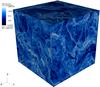 |
Fig. 7 Visualization of the denstrophy Ω1/2 for the same snapshot as in Fig. 6. |
| In the text | |
|
Fig. 8 Correlation diagrams of the SGS turbulence energy vs. the denstrophy, normalized by the cutoff scale Δ, for 5123 LES with solenoidal and compressive forcing. The contours are logarithmic. The average relation between both quantities is indicated by the dotted lines, and the dashed line shows the relation Ksgs ~ 0.1Δ2Ω1/2. |
| In the text | |
|
Fig. 9 Phase diagrams of the effective pressure defined by Eq. (6) vs. the mass density for 5123 LES with solenoidal and compressive forcing. The contours are logarithmic. The averages of the SGS turbulence energy for particular values of the denstrophy are indicated by the dotted lines. |
| In the text | |
|
Fig. 10 Correlation diagrams of the normalized rate of energy dissipation defined by Eq. (36), where νΔ assumes a constant value that is given by the numerical Reynolds number, vs. the rate of energy dissipation (10) that is predicted by the SGS model. The averages of expression (36) for given values of ϱϵsgs are indicated by the dotted lines. |
| In the text | |
|
Fig. 11 Temporal evolution of the rms Mach number (top) and the mean SGS turbulence Mach number (bottom) for solenoidal (left column) and compressive forcing (right column). The cutoff length Δ decreases from L/32 (light colour) to L/256 (full colour). |
| In the text | |
|
Fig. 12 Scaling laws for the mean SGS turbulence Mach number a) and energy b) as functions of the numerical resolution Δ. |
| In the text | |
|
Fig. 13 Temporal evolution of the SGS turbulence energy (top) and the dissipation rate (bottom) for solenoidal (left column) and compressive forcing (right column). The cutoff length Δ decreases from L/32 (light colour) to L/256 (full colour). |
| In the text | |
|
Fig. 14 Left panel: time evolution of the mean internal energy for forcing with varying ζ and about the same rms Mach number. Right panel: volume fractions of zones, in which the SGS turbulence Mach number is greater than any given value for the same forcing parameters as in the left panel (the curves for ζ = 1 and ζ = 2/3 almost coincide). |
| In the text | |
|
Fig. 15 Volume fractions of zones, in which the SGS turbulence Mach number is greater than a certain value for different numerical resolutions. The dashed lines follows from the filtering of 10243 ILES data with filter length 16Δ. This corresponds to the 643 LES, for which Δ/L = 1/32. |
| In the text | |
|
Fig. 16 Temporal evolution of the SGS turbulence Mach number (top) and energy (middle) and the dissipation rate (bottom) for ζ = 2/3 (left column) and ζ = 1/3 (right column). The different lines in each plot correspond to different forcing magnitudes (see Table 5), which are specified by the values of the characteristic Mach number Ma = V/c0 (c0 is the initial speed of sound). |
| In the text | |
|
Fig. 17 Volume fractions of zones, in which the SGS turbulence Mach number is greater than any given value for different rms Mach numbers and mixtures of solenoidal and compressive modes, as in Fig. 16. |
| In the text | |
Current usage metrics show cumulative count of Article Views (full-text article views including HTML views, PDF and ePub downloads, according to the available data) and Abstracts Views on Vision4Press platform.
Data correspond to usage on the plateform after 2015. The current usage metrics is available 48-96 hours after online publication and is updated daily on week days.
Initial download of the metrics may take a while.