| Issue |
A&A
Volume 528, April 2011
|
|
|---|---|---|
| Article Number | A5 | |
| Number of page(s) | 10 | |
| Section | Stellar structure and evolution | |
| DOI | https://doi.org/10.1051/0004-6361/201014457 | |
| Published online | 16 February 2011 | |
The period and amplitude changes in the coolest GW Virginis variable star (PG 1159-type) PG 0122+200
1
Laboratoire d’Astrophysique de Toulouse-Tarbes, Université de Toulouse,
CNRS,
14 Av. E. Belin,
31400
Toulouse,
France
e-mail: This email address is being protected from spambots. You need JavaScript enabled to view it.
2
Department of Astronomy, Beijing Normal University,
100875
Beijing, PR
China
3
Institute of Theoretical Astrophysics, University of Oslo,
PO Box 1029,
Blindern, 0315
Oslo,
Norway
4
Korea Astronomy and Space Science Institute,
San 61-1, Hwaam,
Yuseong, 305-348
Daejeon,
Korea
5
LESIA, Observatoire de Paris-Meudon, Meudon, France
6
Department of Physics and Space Sciences & SARA
Observatory, Florida Institute of
Technology, Florida
32901,
USA
7
Konkoly Observatory, PO Box 67, 1525
Budapest,
Hungary
8
Facultad de Ciencias Astronómicas y Geofísicas, Universidad
Nacional de La Plata, Observatorio-Paseo del Bosque S/N, B1900 FWA La
Plata, Argentina
Received:
18
March
2010
Accepted:
21
December
2010
Abstract
Context. The PG 1159 pre-white dwarf stars experiment a rapidly cooling phase with a time scale of a few 106 years. Theoretical models predict that the neutrinos produced in their core should play a dominant role in the cooling, mainly at the cool end of the PG 1159 sequence. Measuring the evolutionary time scale of the coolest PG 1159 stars could offer a unique opportunity to empirically constrain the neutrino emission rate.
Aims. A subgroup of the PG 1159 stars are nonradial pulsators, the GW Vir type of variable stars. They exhibit g-mode pulsations with periods of a few hundred seconds. As the stars cool, the pulsation frequencies evolve according to the change in their internal structure. It was anticipated that the measurement of their rate of change would directly determine the evolution time scale and so constrain the neutrino emission rates. As PG 0122+200 (BB Psc) defines the red edge of the GW Vir instability strip, it is a good candidate for such a measurement.
Methods. The pulsations of PG 0122+200 have been observed during 22 years from 1986 to 2008, through the fast photometry technique. We used those data to measure the rate of change of its frequencies and amplitudes.
Results. Among the 24 identified ℓ = 1 modes, the frequency and amplitude variations have been obtained for the seven largest amplitude ones. We find changes of their frequency of much larger amplitudes and shorter time scales than the one predicted by theoretical models that assume that the cooling dominates the frequency variations. In the case of the largest amplitude mode at 2497 μHz (400 s), its variations are best fitted by a combination of two terms: one long term with a time scale of 5.4 × 10⁴ years, which is significantly shorter than the predicted evolutionary time scale of 8 × 10⁶ years; and one additional periodic term with a period of either 261 or 211 days. Some other mechanism(s) than the cooling must be responsible for such variations. We suggest that the resonant coupling induced within triplets by the star rotation could be such a mechanism. As a consequence, no useful constraints on the neutrino emission rate can presently be derived as long as the dominant mechanism is not properly understood.
Conclusions. The temporal variations in the pulsation frequencies observed in PG 0122+200 cannot be simply attributed to the cooling of the star, regardless of the contribution of the neutrino losses. Our results suggest that the resonant coupling induced by the rotation plays a dominant role which must be further investigated.
Key words: stars: evolution / neutrinos / white dwarfs / stars: oscillations / stars: individual: PG 0122+200
© ESO, 2011
1. Intoduction
The PG 1159 stars form an evolutionary link between the central stars of planetary nebulae and the white dwarf cooling sequence. A fraction of the PG 1159 stars do pulsate, according to non-radial g-modes, and constitutes the subgroup of the GW Vir variable stars. The asteroseismology of these variable stars provides invaluable insight into their internal structure and evolutionary status. Among the 17 known GW Vir stars (Quirion et al. 2007), five have been observed with the Whole Earth Telescope network (WET; Nather et al. 1990). PG 0122+200 (BB Psc) is the coolest one. Its atmospheric parameters Teff = 80 000 K ± 4000 K, log g = 7.5 ± 0.5, and abundances (C/He = 0.3, C/O = 3, N/He = 10-2 by numbers) are typical of the GW Vir stars (Dreizler & Heber 1998). At this effective temperature, PG 0122+200 presently defines the red edge of the GW Vir instability strip (Quirion et al. 2007). O’Brien et al. (1998) and O’Brien & Kawaler (2000) have shown that, at this phase of the pre-white dwarf evolution, the neutrino losses become important in the cooling process. For a 0.60 M⊙ PG 1159 star at the effective temperature of PG 0122+200, they estimate that the ratio of the neutrino luminosity over the photon luminosity could be 1 ≤ Lν/Lγ ≤ 2.
Since the frequencies of the g-mode pulsations are determined by the internal structure of the star, mainly through the Brunt-Väisälä frequency, the changes in the structure induced by the evolution translate into changes in the pulsation frequencies. The evolution time scale is therefore printed in the changes of the pulsation frequencies. Measuring their rate of change offers an opportunity to estimate the cooling time scale and the importance of the role played by the neutrinos. This makes PG 0122+200 particularly interesting for studying neutrino physics if one could measure its cooling rate from asteroseismology. This was one of the main goals of the follow-up observations of the star.
The predicted neutrino luminosity depends on the stellar parameters, mainly the total mass and the effective temperature, which can, in principle, be determined precisely from asteroseismology. Determining the stellar parameters of a non-radial g-mode pulsator relies on the ability to measure the period spacing between a large enough number of pulsation modes and to correctly identify their degree ℓ (Kawaler & Bradley 1994; Córsico & Althaus 2006). In the best case, a detailed comparison of the observed frequencies with those of realistic models provides an even more precise estimate of the stellar parameters (Kawaler & Bradley 1994; Córsico & Althaus 2006; Córsico et al. 2007).
Discovered as a GW Vir variable star by Bond & Grauer (1987), PG 0122+200 was observed more intensively in 1986 (O’Brien et al.
1996) and then, through a number of multisite
campaigns in 1990 (Vauclair et al. 1995), in 1996
when it was the priority target of a WET campaign (O’Brien et al. 1998), as well as in 2001 and 2002 (Fu et al. 2007). From the cumulative pulsation periods observed during these
campaigns, it was possible to identify 23 periods as ℓ = 1 modes, composed
of seven triplets and two single modes, and to derive a precise value of the average period
spacing, ΔP = 22.9 s (Fu et al. 2007). These results were used by Córsico et al. (2007) to derive precise constraints on the PG 0122+200 parameters, where the most
important ones for estimating the neutrino luminosity are the total mass
 and the effective
temperature (Teff = 81540 (+800, –1400) K) or, alternatively,
the luminosity
(log (L∗/L⊙) = 1.14 (+0.02,
–0.04)). Additional data obtained more recently in 2005 and 2008 are discussed below. We
used all the available data to determine the rate of change of the pulsation frequencies and
of their amplitude.
and the effective
temperature (Teff = 81540 (+800, –1400) K) or, alternatively,
the luminosity
(log (L∗/L⊙) = 1.14 (+0.02,
–0.04)). Additional data obtained more recently in 2005 and 2008 are discussed below. We
used all the available data to determine the rate of change of the pulsation frequencies and
of their amplitude.
This paper is organized as follows. The results of the two new campaigns are described in Sect. 2. Section 3 gives the results on the rate of change of the pulsation frequencies and of their amplitude for the seven largest amplitude modes, including two complete triplets and one component of a third triplet. In Sect. 4 we discuss these results and show that the observed rates of change of the frequencies do not agree with the theoretical prediction based on a neutrino-dominated cooling. We propose another interpretation in terms of resonant coupling induced by rotation. We discuss in more detail the case of the largest amplitude mode, which shows interesting periodic variation in its frequency and amplitude. Section 5 gives a summary and the main conclusions.
2. Results of the 2005 and 2008 multisite campaigns
We conducted two new campaigns on PG 0122+200 in 2005 and 2008. Table 1 gives the journal of the observations for the 2005 campaign, which involved the 2.16-m telescope of the National Astronomical Observatories of China (NAOC) in Xinglong (XL), the 1.8-m telescope of the Bohyunsan Optical Astronomy Observatory (BOAO), and the 0.9-m telescope of SARA at Kitt Peak National Observatory, all for the period from October 1 to October 7, 2005. Additional data were gathered from the 2.56-m Nordic Optical Telescope (NOT) somewhat later from October 14 to 17. All data were acquired with a CCD photometer except in Xinglong where we used a 3-channel photometer. A short description of the 3-channel photometer is given in Vauclair et al. (1989). The sampling rate was 30 s with the CCDs and 1 s with the 3-channel photometer, whose data were summed up to get a similar 30 s sampling rate. During the central part of the campaign (October 1–7), we got 53.2 h of nonoverlapping data during 5.85 days. This corresponds to a duty cycle of 38% and a frequency resolution of ≈ 2 μHz. The additional data from the NOT contributed to significantly improving the length of the campaign to 16.33 days and the corresponding frequency resolution to 0.7 μHz. The duty cycle of the global campaign was 21%. Figure 1 shows the light curve of the 2005 campaign. When data overlapping occurs, for instance between the BOAO and the XL data, we chose to keep the timeseries with the best signal/noise ratio. One notes a variation in the pulsation amplitude during the campaign. Figure 2 shows the power spectrum of the light curve between 500 and 4000 μHz. We did not detect any significant signal below 500 μHz or above 4000 μHz. We used the Period04 software (Lenz & Breger 2005) to derive the frequencies, amplitudes, and phases. Figure 3 shows the detailed pre-whitening process. Note the change in the amplitude scale as the prewhitening proceeds. The process is stopped when no additional significant frequency is selected, according to the chosen detection limit. Here, on the basis of a 4σ detection criterion, the process was stopped after the selection of the 10 frequencies listed in Table 3.
Journal of observations: 2005 October.
Interestingly, the 2005 data show two frequencies at 938.767 μHz and 1558.671 μHz not seen before. We checked the data from the different observing sites separately to verify that those frequencies did not come from an instrumental effect on one site. Those frequencies are seen in the power spectrum of all the timeseries. We interpret the 1558.671 μHz (641.6 s period) as a component of one additional ℓ = 1 mode to the series listed in Fu et al. (2007) in which the lowest frequency mode was at 1636.25 μHz (611.15 s). This new mode corresponds to the k = 25 order, ℓ = 1 mode of the best-fit model of Córsico et al. (2007), which is found at 633.1 s; however, we detect only one frequency, so we do not know its m value. With this additional mode, the periods observed in PG 0122+200 cover a total range of 336 s to 642 s. This is in good agreement with the range of unstable ℓ = 1 modes found in the best-fit model of Córsico et al. (2007). From this model, all the modes observed in PG 0122+200 are predicted to be unstable. This is also in good agreement with the periods of the unstable modes in the closest model to PG 0122+200 in the evolutionary sequence of Quirion et al. (2007, their Table 5), which covers a range of 232 s to 587 s.
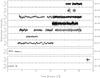 |
Fig. 1 Normalized light curve of PG 0122+200 during the 2005 campaign. The fractional modulated intensity, indicated on the left side, is plotted as a function of time (UT). Each panel covers a 24 h period; the date is indicated on the right side. |
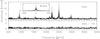 |
Fig. 2 Amplitude spectrum of the 2005 light curve. The upper panel shows the amplitude spectrum in units of milli-modulation amplitude (mma) as a function of the frequency in μHz, in the frequency range 500–4000 μHz; no significant signal is detected outside this frequency range. The corresponding window function is shown on the same scale in the insert. The lower panel shows the residuals after subtraction of the 10 significant frequencies detected. |
The peak at 938.767 μHz (1065.2 s period) appears when the 1558.671 μHz peak is also present. Its frequency is very close to a linear combination of the dominant frequency at 2497 μHz with the 1558 μHz one (2497 μHz–1558 μHz = 939 μHz). However, such linear combinations and/or harmonics of genuine eigenfrequencies are seen when a significant outer convective zone interacts with the pulsations as in the case of the DBVs (for instance GD 358, Provencal et al. 2009) and the cool DAVs (for instance HL Tau 76, Dolez et al. 2006). Because there is no such significant outer convective region in the PG 1159 stars, one does not expect to see any signature of convection-pulsation interactions. In fact, no linear combinations of frequencies have been detected so far in PG 0122+200 or in the PG 1159 prototype star PG 1159-035 (Costa et al. 2008). In addition, we also note that the 2005 data do not show any significant signal at 2497 μHz + 1558 μHz = 4055 μHz. We conclude that the peak at 938.767 μHz does not result from a linear combination. Inspection of the best-fit model of Córsico et al. (2007) reveals that the ℓ = 1, k = 43 mode has a period of 1063.8 s, very close to the observed one. However, according to their nonadiabatic computations, this mode is predicted to be stable. We conclude that this peak at 938.767 μHz could correspond to a genuine mode excited by resonance with the two unstable modes at 2497 μHz and 1558 μHz. In contrast, the best-fit model does not show any eigenfrequency close to 4055 μHz: the closest (unstable) ℓ = 1 modes are the k = 8 at 4210 μHz and the k = 9 at 3771.7 μHz.
The 2008 campaign involved the 2.16-m telescope of NAOC in Xinglong (XL), the 1.8-m telescope of BOAO and the 1-m telescope on the station of Konkoly Observatory at Piszkéstető. Table 2 gives the journal of the observations for the 2008 campaign. Again, data were obtained with CCD photometers except at Xinglong where we used the 3-channel photometer. The set-up was the same as in 2005. We got 56.4 h of nonoverlapping data during a campaign of 8.02 days, which gives a duty cycle of 29% and a frequency resolution of 1.4 μHz. Figures 4–6 show the light curve, the power spectrum, and the detailed pre-whitening process, respectively. Using the same 4σ detection criterion, we detect 13 significant frequencies in the 2008 data set. The additional frequencies detected in 2005 at 938.767 μHz and 1558.671 μHz do not show up in the 2008 data.
As a summary, with the addition of the new data obtained in 2005 and 2008, PG 0122+200 shows 24 unstable modes. It also occasionally shows a stable mode excited by resonance with two unstable modes, as observed during the 2005 campaign.
The frequencies detected during the 2005 and 2008 campaigns are listed in Table 3, where σ are the uncertainties on the derived frequencies and A their amplitude expressed in milli-modulation amplitude (mma). The quoted frequency uncertainties are the internal errors derived from Period04. They are known to underestimate the true uncertainties. Section 3 describes how we derive more realistic frequency uncertainties to estimate the rates of change of the frequencies and discuss their significance.
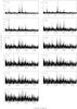 |
Fig. 3 Illustration of the prewhitening process on the 2005 amplitude spectrum. The first panel (FT01) is the full amplitude spectrum as shown in Fig. 2. Panel FT02 shows the amplitude spectrum after subtraction of the largest amplitude peak at 2497 μHz. The next panel (FT03) shows the amplitude spectrum after additional subtraction of the next largest amplitude peak at 2221 μHz, and so on for the subsequent panels. |
Journal of observations: 2008 October.
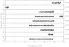 |
Fig. 4 Same as Fig. 1 for the 2008 campaign. |
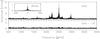 |
Fig. 5 Same as Fig. 2 for the 2008 light curve. Here the lower panel shows the residuals after subtraction of the 13 significant frequencies detected. |
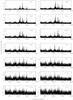 |
Fig. 6 Same as Fig. 3 for the 2008 amplitude spectrum. Here, 13 significant frequencies are selected according to the chosen detection limit, as listed in Table 3. |
Frequencies in PG 0122+200 during the 2005 and 2008 campaigns.
3. The rate of change of the pulsation frequencies
In addition to the new data obtained in 2005 and 2008 described above, we have reanalyzed the data obtained since 1986 and redetermined the frequencies, the amplitudes, and the phases in a homogenous way by using the Period04 software (Lenz & Breger 2005). Since the uncertainties derived by Period04 only estimate the internal consistency of the solutions, they are underestimated. We derived more realistic uncertainties through Monte-Carlo simulations.
For each observed timeseries (ti,xi)i = 1,2,...,k, we extracted a number of frequencies (fj)j = 1,2,...,n and the corresponding amplitudes Aj and phases φj with the software Period04, so the residual time-series (ti,yi)i = 1,2,...,k were obtained by subtracting the sum of multiple sine functions from the observed timeseries as
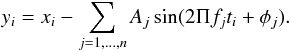 Then
| yi | is regarded as the observation error
of xi. Hence, we constructed 50 simulated
time-series zi for each observed time-series,
by taking zi as a normally distributed random
variable with mean xi and standard variation
| yi | . The 50 simulated time-series were
fitted with the sum of multiple sine functions by taking
(fj,Aj,φj)j = 1,2,...,n
as initial values according to least-squares algorithm. Hence 50 sets of new
(fj,Aj,φj)j = 1,2,...,n
were obtained. The standard deviations of each parameter of
(fj,Aj,φj)j = 1,2,...,n
were then calculated. We define them as the uncertainty estimates of the parameters.
Then
| yi | is regarded as the observation error
of xi. Hence, we constructed 50 simulated
time-series zi for each observed time-series,
by taking zi as a normally distributed random
variable with mean xi and standard variation
| yi | . The 50 simulated time-series were
fitted with the sum of multiple sine functions by taking
(fj,Aj,φj)j = 1,2,...,n
as initial values according to least-squares algorithm. Hence 50 sets of new
(fj,Aj,φj)j = 1,2,...,n
were obtained. The standard deviations of each parameter of
(fj,Aj,φj)j = 1,2,...,n
were then calculated. We define them as the uncertainty estimates of the parameters.
With all the observed light curves available, we were able to follow the frequency and amplitude variations by the direct measurements for the 7 largest amplitude modes. This includes the three components of the triplets at 2221, 2224, 2228 μHz and at 2490, 2493, 2497 μHz and the prograde component of a third triplet at 2973 μHz. The list of the measured frequencies and amplitudes of these modes, together with their uncertainties derived from the Monte-Carlo simulations, is given in Table 4. The columns indicate the dates of the measurements in HJD and in year.months, the frequencies and their uncertainties, σ, the amplitudes A and their uncertainties δA.
The other modes either do not show up in a large enough number of observations or have too low amplitudes for a significant detection of frequency variations. The frequency variations of the 3 components of the first triplet at 2221, 2224, 2228 μHz are shown in Fig. 7. Figure 8 shows the corresponding amplitude variations of the three components. Figures 9 and 10 show the frequency variations and the corresponding amplitude variations, respectively, for the three components of the second triplet at 2490, 2493, 2497 μHz. Figures 11 and 12 show the frequency and amplitude variations for the prograde component of the third triplet at 2973 μHz. In those figures the time is expressed in heliocentric Julian days (HJD) rather than in barycentric Julian days (BJD). This does not affect our analysis since the pulsation frequencies are determined independently for each run. Among these seven modes, only the largest amplitude ones, at 2221 μHz, 2497 μHz, and 2973 μHz, are present in all the observing campaigns. Since the variations are clearly nonlinear with time, the (O − C) method is difficult to use in this case.
Frequency and amplitude variations of the 7 largest amplitude modes in PG 0122+200 measured from 1986 to 2008.
As can be seen from the various figures, the behavior of the variations varies for different frequencies. The frequency variations are much larger than expected from the model predictions, which are based on the assumption that the cooling, possibly dominated by neutrino luminosity, is the unique cause of the frequency changes. We observe frequency variations of a fraction of μHz instead of the predicted 10-3 μHz, which would have been impossible to observe with the present data. This implies frequency variations on time scales of a few 104 years, considerably shorter than the cooling time scale of a few 106 years derived from the currently most elaborated theoretical model (Córsico et al. 2007).
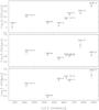 |
Fig. 7 Temporal changing of the frequency for the three components of the triplet centered at 2224 μHz. For each of the components, the difference between the full frequency and its integer value, noted on the ordinates as FREQ [– integer value], is plotted as function of time in HJD, referred to as 2446000.0. The dates of the observations are marked for each data point as yyyy.mm. Error bar for each data set is derived from Monte-Carlo simulations. |
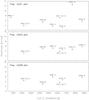 |
Fig. 8 Temporal changing of the amplitude for the three components of the triplet centered at 2224 μHz. For each of the components, the amplitude in mma is plotted as function of time in HJD, referred to as 2446000.0. The dates of the observations are marked for each data point as yyyy.mm. Error bar for each data set is derived from Monte-Carlo simulations. |
4. Interpretations
4.1. The rate of change of the pulsation frequencies predicted by theoretical models
The evolutionary model by Córsico et al. (2007) relies on the neutrino production rate by Itoh et al. (1989, 1992). The estimated cooling time scale of the O’Brien & Kawaler’s evolutionary models (2000) is based on the updated neutrino emission rate of Itoh et al. (1996). However, there is no significant difference in the cooling time scale or in the rate of period changes by using one or the other version of the neutrino emission rate. According to the predictions of the Córsico’s best-fit model, the rate of change of the pulsation periods (Ṗ = dP/dt) varies between 1.22 × 10⁻¹² s s-1 for the ℓ = 1, k = 12 mode of period 336.68 s and 3.26 × 10⁻¹² s s-1 for the ℓ = 1, k = 24 mode of period 611.15 s. These values translate into evolutionary time scales between 8.7 × 10⁶ and 5.9 × 10⁶ years. On the twenty-two year time scale covered by the observations reported here, one should not have detected frequency variations greater than –7.5 × 10⁻³ μHz ≤ δf ≤ –6.1 × 10⁻³ μHz (i.e. 8.4 × 10⁻⁴ s ≤ δP ≤ 2.3 × 10⁻³ s in the period variations). Such small variations are not reachable within 22 years given the present uncertainties on the frequency determination. We estimate that it would take more than 50 years to get a significant 3-σ signature of a frequency change induced by the cooling.
All of the seven largest amplitude modes of pulsation for which we have estimated a rate of change of their frequency are trapped modes according to the Córsico’s best-fit model. As a consequence, the rate of change of their frequency should be a combination of the star cooling and of the outer layers final contraction. The rates of change of the theoretical ℓ = 1, m = 0 modes listed in Córsico et al. (2007) for the radial orders k between 12 and 24 covering the range of observed periods, are all positive (see their Table 1). It means that the rates of change are dominated by cooling and that the contraction of the outer layers has little effect. However, as can be inferred from their Table 1, the rates of changes for the trapped modes are less than for the untrapped modes, indicating a small effect from the outer layers.
As can be seen from Figs. 7, 9, and 11, the frequency variations of these modes show irregular patterns. The only mode showing a frequency variation consistent with a flat behavior is the prograde component of the third triplet at 2973 μHz. Figure 12 also shows that its amplitude remains almost constant during the 22 years covered by our data. This suggests that this mode is stable enough in frequency and in amplitude to be used to measure the neutrino emission rate if one could get more data. A second-order polynomial fit to the data shown in Fig. 11 indicates, however, a time scale of 7.8 ± 6.0 × 10⁵ y. With a difference of 13σ, this is one order of magnitude shorter than the cooling time scale of 8.7 × 10⁶ y derived by Córsico et al. (2007) for this mode. Furthermore, Fig. 11 shows a frequency increasing (period decreasing) with time, while in the Córsico’ best-fit model the period derivative for this mode is positive, indicating a period change dominated by cooling. At this stage we conclude that either the role of the envelope contraction is underestimated in the evolutionary models used to estimate the rate of period change, or another physical mechanism is dominating the frequency variation. This is discussed below.
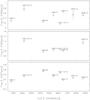 |
Fig. 9 Same as Fig. 7 for the components of the triplet centered at 2493 μHz. |
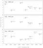 |
Fig. 10 Same as Fig. 8 for the components of the triplet centered at 2493 μHz. |
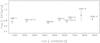 |
Fig. 11 Same as Fig.7 for the prograde component of the triplet centered at 2970 μHz. |
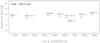 |
Fig. 12 Same as Fig. 8 for the prograde component of the triplet centered at 2970 μHz. |
4.2. The rate of change of the pulsation frequencies in PG 0122+200 and a comparison with those in PG 1159-035
The results presented here show that the observed frequency variations are one to two orders of magnitude larger than the ones derived from the best-fit model of Córsico et al. (2007) and they do not follow a simple function of time. Their typical time scales are much shorter than the expected cooling time, for any reasonable assumption on the rate of neutrino production.
Similar results have been obtained for the prototype of the GW Vir pulsators PG 1159-035 (Costa & Kepler 2008). In this case, the period changes have been estimated for 27 modes. However, only two modes were detected at five different seasons, five at four different seasons and the remaining 20 were only detected at three different seasons. About half of the modes show increasing periods and half show decreasing ones. Two of the modes that are identified as trapped modes in the best-fit model of Córsico et al. (2008) show decreasing periods, as expected. The dominant mode at 516 s shows a regularly increasing period. But the time scale inferred from its variation (1.3 × 10⁵ y) is one order of magnitude shorter than the one predicted by the Córsico’ model for this mode. Among the other modes, different types of variation are observed; in particular two of them, at 451.5 s and 536.9 s, show large negative and positive frequency variations on short time scales.
However, the case of PG 1159-035 is substantially different from the case of PG 0122+200. The star PG 1159-035 appears to still be in the “evolutionary knee”, a stage in which the He shell burning is an important source of luminosity that controls the evolutionary timescale and thus the rate of period change. At variance, PG 0122+200 is located at a stage where (according to theoretical models) the He shell burning has been virtually extinct. The disagreement between the cooling time scale derived from evolutionary models of PG 1159-035 and the observed time scales of the period changes has been recently solved by Althaus et al. (2008). They show that the magnitude and sign of the rates of period changes observed in that star by Costa & Kepler (2008) could be reconciled with the theoretical models if the star were characterized by a thinner He-rich envelope, so as to be incapable of sustaining He shell burning. In this way, the rates of period changes should be higher (and the evolutionary time scale shorter) by one order of magnitude, in agreement with the observational demand. But this solution is not valid for PG 0122+200, because for the regime of this star, the He burning is no longer the luminosity source, so the magnitude of the period changes becomes much less sensitive to the thickness of the He envelope. One has to find another explanation for the period-change time scales in PG 0122+200 being much shorter than the expected cooling time scale.
4.3. Which mechanism?
Our results on PG 0122+200 indicate that the observed frequency variations are not dominated by cooling. They are not induced by an orbiting companion either, i.e. a planet or a brown dwarf, in contrast to the case of the sdB pulsator V391 Peg (Silvotti et al. 2007), since the variations in different frequencies are not correlated in phase and do not have the same amplitudes and time scales. We have to think about other mechanism(s). One potential mechanism producing such frequency and amplitude variations is the resonant coupling induced by rotation within triplets, as discussed by Goupil et al. (1998). They showed that, in order of magnitude, the effect of such resonant coupling depends on the value of the parameter D = 2πδf/κ0 measuring the ratio of the frequency mismatch induced in a triplet by second-order effect of rotation (δf) and the mode growth rate (κ0). According to its value, one may encounter three different regimes. If this ratio is low, the frequencies are forced to be equally spaced within the triplet; this is the frequency lock regime. If the ratio is high, the resonant coupling is inefficient and the frequencies keep their nonresonant properties, i.e. keep their linear values. In the intermediate case, both the amplitudes and the frequencies undergo time modulation with typical time scale Pmod ≈ 1/δf. The variations observed in PG 0122+200 suggest that many of the modes could be in this intermediate regime. A detailed comparison of the frequency and amplitude variations observed in PG 0122+200 with the predictions of the nonlinear pulsation theory would probably require more observational data and theoretical investigations of the resonant coupling mechanism.
4.4. Rotational splitting revisited
Since we argue that the observed frequency variations are due to the resonant coupling induced by second-order effect of rotation, the frequency shifts observed within the triplets do not only measure the rotation rate. They also include a contribution due to this resonant coupling. By time averaging the frequency shifts observed at different seasons, one should minimize that contribution and get a better estimate of the part only due to the first order of rotation. We performed this time average on the triplets centered at 2493 μHz and at 2224 μHz corresponding to modes k = 15 and 17 respectively in the best-fit model of Córsico et al. (2007). The resulting averaged rotational splitting of 3.405 μHz translates into an average rotation period of 1.70 days. This is a slightly longer rotation period than the 1.55 days found by Fu et al. (2007). In addition, the nonlinear effect invoked by Goupil et al. (1998) also implies a time modulation of the departure to equal splitting within the triplets in the intermediate regime. Considering the case of the two triplets illustrated in Figs. 7 and 9 we find such a time modulation. This is shown in Fig. 13 for the triplet centered at 2224 μHz and in Fig. 14 for the triplet centered at 2493 μHz. The three components of the triplets are not always detected. In the case of these two triplets, they are seen simutaneously during six observing seasons. Each figure shows the variations in the frequency shift for the retrograde and the prograde components of the triplets. The departure to equal splitting and its time modulation are clearly visible.
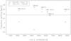 |
Fig. 13 Time modulation of the frequency shifts of the retrograde (m = − 1) and prograde (m = + 1) components of the triplet centered at 2224 μHz. The frequency shift f(m = 0) – f(m = − 1) for the retrograde component ( × ) and f(m = + 1) – f(m = 0) for the prograde component (o) are plotted as function of time, relatively to their average value marked by the continuous horizontal line. |
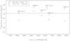 |
Fig. 14 Same as Fig. 13 for the triplet centered at 2493 μHz. |
4.5. The case of the dominant mode at 2497 μHz
The mode at 2497 μHz has always been the one with the largest amplitude in all of the eight observing seasons reported here. It is the prograde component (m = + 1) of the triplet centered at 2493 μHz. Its frequency variations, shown in the lower panel of Fig. 9, suggests a periodic oscillation, particularly visible within the period 1996–2008 during which we got six observational points. As this behavior could shed some light on the physical mechanism responsible for the frequency and amplitude variations, we explored this case further. A second-order polynomial is subtracted from the frequency data points as shown in the upper panel of Fig. 15. The residuals, shown in the middle panel, are then fitted by a one-component sine function by a χ2 minimization. Since there are only eight observing seasons on the 22 years of observation, these fits cannot constrain the period of the modulation with a unique value. We explored a rather wide range of possible periodicity, between 120 and 360 days. Within this range of periodicities, χ2 varies between 0.137 and 0.014. We find 12 secondary minima with 0.014 ≤ χ2 ≤ 0.047. The best χ2 values are obtained for periodicity of 261.0 days (0.018), 212.6 days (0.016), and 130.5 days (0.014), which is half of the 261.0 days period as expected. As the resonant coupling mechanism should induce a time modulation with the same periodicity for both the frequency and the amplitude, we did the same treatment to the amplitude data points. A second-order polynomial is fitted to the data as shown in the upper panel of Fig. 16. The residuals are fitted with one-component sine functions with periods covering the same range as for the frequency fits. The χ2 values vary between 28.7 and 1.0 and show 15 secondary minima with 1.0 ≤ χ2 ≤ 8.8. The best χ2 values are found for periodicities of 260.9 days (1.8), 210.2 days (1.0), 151.5 days (1.8), and half of the 260.9 days at 130.5 days (3.6). The two lower χ2 minima in common in the frequency and amplitude fits are not significantly different in terms of χ2. The corresponding periodicities are 211 days and 261 days, respectively. In the middle panels of Figs. 15 and 16, we show the fit of the residuals with the sine function of period 211 days. Such modulation periods have the right order of magnitude as predicted by Goupil et al. (1998).
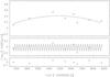 |
Fig. 15 Upper panel: the 2497 μHz frequency variations fit with a second-order polynomial; middle panel: the residuals fit with a one-component sine function with a period of 211 days; lower panel: the final residuals. |
This analysis suggests that there are two different time scales in the frequency and amplitude variations. For the frequency variation, one long-term time scale is deduced from the polynomial fit. Its value τf = [(1/f)(df/dt)] -1 of 5.4 × 10⁴ years has to be compared with the theoretical prediction of 8.0 × 10⁶ years for the m = 0 mode of this triplet from the best-fit model of Córsico et al. (2007). We assume here that the frequency rate of change of the rotationally split components do not significantly differ from the one estimated for the central m = 0 component of the triplet. The observed rate of change disagrees with the theoretical prediction by a factor 150. The second-order polynomial fit of the amplitude variations shows an increase in the amplitude with a time scale τamp = [(1/ ⟨A⟩)(dA/dt)] -1, where ⟨ A ⟩ is the average amplitude, of 6.1 × 10⁵ years.
As a result, the long-term time scale of the frequency variations for the dominant mode is much shorter, by two orders of magnitude, than the evolutionary time scales evaluated with the above-mentioned neutrino emission rates. It is quite improbable that the neutrino emission rates of Itoh et al. (1989, 1992, 1996) are underestimated by two orders of magnitude. We presently have no explanation to this discrepancy.
We attribute the other, short-term component in the frequency and amplitude variations to the effect of the resonant coupling induced by rotation. The sine function that fits the residuals shown in the middle panels of Figs. 15 and 16 has a period of 211 days and an amplitude of 0.11 μHz in frequency and of 1.9 mma in amplitude, respectively. The other equivalent χ2 solution with a 261 days period has an amplitude of 0.12 μHz in frequency and of 1.7 mma in amplitude.
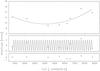 |
Fig. 16 Upper panel: the 2497 μHz amplitude variations fit with a second-order polynomial; middle panel: the residuals fit with a one-component sine function with a period of 211 days; lower panel: the final residuals. |
5. Summary and conclusions
The available asteroseismological observations of PG 0122+200 cover a period of 22 years from 1986 to 2008. The two most recent observational campaigns in 2005 and 2008 are reported here. These new data allowed us to discover one additional unstable mode with a period in excellent agreement with the ℓ = 1, k = 25 mode of the best-fit model of Córsico et al. (2007). This increases to 24 the number of modes available for an asteroseismic analysis. In addition, we find evidence, for the first time, of one stable mode showing up in the 2005 data, excited by resonance with two unstable modes. All the data were reanalyzed in a homogeneous way to derive the frequencies and the amplitudes of the pulsation modes. Monte-Carlo simulations were used to obtain realistic estimates of their uncertainties.
We measured the frequency and amplitude variations for the seven largest amplitude modes. Our initial goal was to derive the evolutionary time scale from the rate of change of the pulsation frequencies. Since PG 0122+200 is predicted to cool predominantly by neutrino losses, the measure of the evolutionary time scale was supposed to provide constraints on the efficiency of the neutrino production.
We find that the frequencies vary on time scales that are one to two orders of magnitude shorter than the ones derived from the best-fit model of Córsico et al. (2007) and that they do not follow a simple function of time. They are much shorter than the expected cooling time, for any reasonable assumption on the rate of neutrino production.
A similar disagreement between the time scales derived from the observed rates of change of the pulsation frequencies and the theoretical cooling time in the prototype of the GW Vir pulsators PG 1159-035 (Costa & Kepler 2008) has been solved by model of PG 1159-035 with an He envelope 2–3 times thinner than the usual canonical value (Althaus et al. 2008). But the same argument does not help for understanding the case of PG 0122+200, which is much cooler and in which the He envelope thickness has much less influence on the evolutionary time scale.
These results indicate that the observed frequency variations are not dominated by cooling. One potential mechanism producing such frequency and amplitude variations is the resonant coupling induced by rotation within triplets, as discussed by Goupil et al. (1998). The frequency and amplitude variations observed in PG 0122+200 suggest that most of the pulsation modes could be in an intermediate regime where both the frequency and the amplitude are time-modulated. We took the contribution of this effect into account to revisit the rotational splitting and derive a new rotation period of 1.70 days.
In PG 0122+200, the frequency variations observed for the largest amplitude mode at 2497 μHz show an interesting periodic behavior that we have investigated further as it may provide some hints on the mechanism behind the frequency and amplitude variations. The frequency variations of this mode may be decomposed into two components: a long-term one with a time scale of 5.4 × 10⁴ years and a periodic short-term with a period of either 261 or 211 days.
This is the first estimate of the modulation time scale induced by the resonant coupling mechanism. We note, however, that the long-term time scale is 150 times shorter than the theoretical predicted evolutionary time scale. Unless the neutrino emission rates used in the evolutionary models are underestimated by one to two orders of magnitude, which seems unlikely, this indicates that the frequency variations are not dominated by the star cooling.
Our results for PG 0122+200 do not allow one to constrain the neutrino emission rate and its efficiency on the cooling time scale. It has been argued that at the luminosity of the DB variable white dwarfs, the neutrino losses play also an important role in the cooling. Measuring the rate of change of their pulsation periods could constrain the neutrino emission rate (Winget et al. 2004; Sullivan et al. 2008), unless those period changes are subject to the same resonant coupling mechanism as observed in PG 0122+200.
These intriguing results suggest that we are missing some dominant physical processes either in the pulsation theory or in the cooling theory, or else in both. In this direction, some more theoretical work is needed to investigate further the relevance of the mechanism suggested by Goupil et al. (1998).
Acknowledgments
We thank the referee whose suggestions contributed to improve an earlier version of the manuscript. G.V., N.D., and M.C. acknowledge financial support from “Programme National de Physique Stellaire” (PNPS) of CNRS/INSU, France and from Natural Science Foundation of China (NSFC) under the grant number 10673001. J.N.F. acknowledges financial support from Natural Science Foundation of China (NSFC) under the grant numbers 10878007 and 10778601. A.H.C. acknowlegdes support of AGENCIA: Programa de Modernización Tecnológica BID 1728/OC-AR. Based on observations made with the 2.16-m telescope at Xinglong station of China, which is operated by National Astronomical Observatories of Chinese Academy of Sciences, the 1.8-m telescope of the Bohyunsan Optical Astronomical Observatory, the 1-m telescope of the Konkoly Observatory, the 0.9-m telescope of SARA at Kitt Peak National Observatory and the Nordic Optical Telescope, operated on the island of La Palma jointly by Denmark, Finland, Iceland, Norway, and Sweden, in the Spanish Observatorio del Roque de los Muchachos of the Instituto de Astrofisica de Canarias. The NOT data presented here have been taken using ALFOSC, which is owned by the Instituto de Astrofisica de Andalucia (IAA) and operated at the Nordic Optical Telescope under agreement between IAA and the NBIfAFG of the Astronomical Observatory of Copenhagen.
References
- Althaus, L. G., Córsico, A. H., Miller Bertolami, M. M., et al. 2008, ApJ, 677, L35 [NASA ADS] [CrossRef] [Google Scholar]
- Bond, H., & Grauer, A. 1987, ApJ, 321, L123 [NASA ADS] [CrossRef] [Google Scholar]
- Córsico, A. H., & Althaus, L. G. 2006, A&A, 454, 863 [NASA ADS] [CrossRef] [EDP Sciences] [Google Scholar]
- Córsico, A. H., Miller Bertolami, M. M., Althaus, L. G., Vauclair, G., & Werner, K. 2007, A&A, 475, 619 [NASA ADS] [CrossRef] [EDP Sciences] [Google Scholar]
- Córsico, A. H., Althaus, L. G., Kepler, S. O., et al. 2008, A&A, 478, 869 [NASA ADS] [CrossRef] [EDP Sciences] [Google Scholar]
- Costa, J. E. S., & Kepler, S. O. 2008, A&A, 489, 1225 [NASA ADS] [CrossRef] [EDP Sciences] [Google Scholar]
- Costa, J. E. S., Kepler, S. O., Winget, D. E., et al. 2008, A&A, 477, 627 [NASA ADS] [CrossRef] [EDP Sciences] [Google Scholar]
- Dolez, N., Vauclair, G., Kleinman, S. J., et al. 2006, A&A, 446, 237 [NASA ADS] [CrossRef] [EDP Sciences] [Google Scholar]
- Dreizler, S., & Heber, U. 1998, A&A, 334, 618 [NASA ADS] [Google Scholar]
- Fu, J.-N., Vauclair, G., Solheim, J.-E., et al. 2007, A&A, 467, 237 [NASA ADS] [CrossRef] [EDP Sciences] [Google Scholar]
- Goupil, M. J., Dziembowski, W. A., & Fontaine, G. 1998, Baltic Astron., 7, 21 [Google Scholar]
- Itoh, N., Adachi, T., Nakagawa, M., et al. 1989, ApJ, 339, 354 [NASA ADS] [CrossRef] [Google Scholar]
- Itoh, N., Mutoh, H., Hikita, A., & Kohyama, Y. 1992, ApJ, 395, 622 [NASA ADS] [CrossRef] [Google Scholar]
- Itoh, N., Hayashi, H., Nishikawa, A., & Kohyama, Y. 1996, ApJS, 102, 411 [NASA ADS] [CrossRef] [Google Scholar]
- Kawaler, S. D., & Bradley, P. A. 1994, ApJ, 427, 415 [NASA ADS] [CrossRef] [Google Scholar]
- Lenz, P., & Breger, M. 2005, Comm. in Asteroseismology, 146, 53 [Google Scholar]
- Nather, R. E., Winget, D. E., Clemens, J. C., Hansen, C. J., & Hine, B. P. 1990, ApJ, 361, 309 [NASA ADS] [CrossRef] [Google Scholar]
- O’Brien, M. S., & Kawaler, S. D. 2000, ApJ, 539, 372 [NASA ADS] [CrossRef] [Google Scholar]
- O’Brien, M. S., Clemens, J. C., Kawaler, S. D., & Dehner, B. T. 1996, ApJ, 467, 397 [NASA ADS] [CrossRef] [Google Scholar]
- O’Brien, M. S., Vauclair, G., Kawaler, S. D., et al. 1998, ApJ, 495, 458 [NASA ADS] [CrossRef] [Google Scholar]
- Provencal, J. L., Montgomery, M. H., Kanaan, A., et al. 2009, ApJ, 693, 564 [NASA ADS] [CrossRef] [Google Scholar]
- Quirion, P.-O., Fontaine, G., & Brassard, P. 2007, ApJS, 171, 219 [NASA ADS] [CrossRef] [Google Scholar]
- Silvotti, R., Schuh, S., Janulis, R., et al. 2007, Nature, 449, 189 [NASA ADS] [CrossRef] [PubMed] [Google Scholar]
- Sullivan, D. J., Metcalfe, T. S., O’Donoghue, D., et al. 2008, MNRAS, 387, 137 [NASA ADS] [CrossRef] [Google Scholar]
- Vauclair, G., Goupil, M. J., Baglin, A., et al. 1989, A&A, 215, L17 [NASA ADS] [Google Scholar]
- Vauclair, G., Pfeiffer, B., Grauer, A., Belmonte, J.-A., et al. 1995, A&A, 299, 707 [NASA ADS] [Google Scholar]
- Winget, D. E., Sullivan, D. J., Metcalfe, T. S., et al. 2004, ApJ, 602, L109 [NASA ADS] [CrossRef] [Google Scholar]
All Tables
Frequency and amplitude variations of the 7 largest amplitude modes in PG 0122+200 measured from 1986 to 2008.
All Figures
|
Fig. 1 Normalized light curve of PG 0122+200 during the 2005 campaign. The fractional modulated intensity, indicated on the left side, is plotted as a function of time (UT). Each panel covers a 24 h period; the date is indicated on the right side. |
| In the text | |
|
Fig. 2 Amplitude spectrum of the 2005 light curve. The upper panel shows the amplitude spectrum in units of milli-modulation amplitude (mma) as a function of the frequency in μHz, in the frequency range 500–4000 μHz; no significant signal is detected outside this frequency range. The corresponding window function is shown on the same scale in the insert. The lower panel shows the residuals after subtraction of the 10 significant frequencies detected. |
| In the text | |
|
Fig. 3 Illustration of the prewhitening process on the 2005 amplitude spectrum. The first panel (FT01) is the full amplitude spectrum as shown in Fig. 2. Panel FT02 shows the amplitude spectrum after subtraction of the largest amplitude peak at 2497 μHz. The next panel (FT03) shows the amplitude spectrum after additional subtraction of the next largest amplitude peak at 2221 μHz, and so on for the subsequent panels. |
| In the text | |
|
Fig. 4 Same as Fig. 1 for the 2008 campaign. |
| In the text | |
|
Fig. 5 Same as Fig. 2 for the 2008 light curve. Here the lower panel shows the residuals after subtraction of the 13 significant frequencies detected. |
| In the text | |
|
Fig. 6 Same as Fig. 3 for the 2008 amplitude spectrum. Here, 13 significant frequencies are selected according to the chosen detection limit, as listed in Table 3. |
| In the text | |
|
Fig. 7 Temporal changing of the frequency for the three components of the triplet centered at 2224 μHz. For each of the components, the difference between the full frequency and its integer value, noted on the ordinates as FREQ [– integer value], is plotted as function of time in HJD, referred to as 2446000.0. The dates of the observations are marked for each data point as yyyy.mm. Error bar for each data set is derived from Monte-Carlo simulations. |
| In the text | |
|
Fig. 8 Temporal changing of the amplitude for the three components of the triplet centered at 2224 μHz. For each of the components, the amplitude in mma is plotted as function of time in HJD, referred to as 2446000.0. The dates of the observations are marked for each data point as yyyy.mm. Error bar for each data set is derived from Monte-Carlo simulations. |
| In the text | |
|
Fig. 9 Same as Fig. 7 for the components of the triplet centered at 2493 μHz. |
| In the text | |
|
Fig. 10 Same as Fig. 8 for the components of the triplet centered at 2493 μHz. |
| In the text | |
|
Fig. 11 Same as Fig.7 for the prograde component of the triplet centered at 2970 μHz. |
| In the text | |
|
Fig. 12 Same as Fig. 8 for the prograde component of the triplet centered at 2970 μHz. |
| In the text | |
|
Fig. 13 Time modulation of the frequency shifts of the retrograde (m = − 1) and prograde (m = + 1) components of the triplet centered at 2224 μHz. The frequency shift f(m = 0) – f(m = − 1) for the retrograde component ( × ) and f(m = + 1) – f(m = 0) for the prograde component (o) are plotted as function of time, relatively to their average value marked by the continuous horizontal line. |
| In the text | |
|
Fig. 14 Same as Fig. 13 for the triplet centered at 2493 μHz. |
| In the text | |
|
Fig. 15 Upper panel: the 2497 μHz frequency variations fit with a second-order polynomial; middle panel: the residuals fit with a one-component sine function with a period of 211 days; lower panel: the final residuals. |
| In the text | |
|
Fig. 16 Upper panel: the 2497 μHz amplitude variations fit with a second-order polynomial; middle panel: the residuals fit with a one-component sine function with a period of 211 days; lower panel: the final residuals. |
| In the text | |
Current usage metrics show cumulative count of Article Views (full-text article views including HTML views, PDF and ePub downloads, according to the available data) and Abstracts Views on Vision4Press platform.
Data correspond to usage on the plateform after 2015. The current usage metrics is available 48-96 hours after online publication and is updated daily on week days.
Initial download of the metrics may take a while.