| Issue |
A&A
Volume 527, March 2011
|
|
|---|---|---|
| Article Number | L7 | |
| Number of page(s) | 4 | |
| Section | Letters | |
| DOI | https://doi.org/10.1051/0004-6361/201016313 | |
| Published online | 02 February 2011 | |
Letter to the Editor
Lyman-α emitters as tracers of the transitioning Universe
1
ST-ECF, Karl-Schwarzschild-Straße 2,
85748
Garching bei München,
Germany
e-mail: knilsson@eso.org
2
European Southern Observatory, Karl-Schwarzschild-Straße 2, 85748
Garching bei München,
Germany
Received:
14
December
2010
Accepted:
15
January
2011
Of all the many ways of detecting high-redshift galaxies, the selection of objects by their redshifted Lyα emission has become one of the most successful. But what types of galaxies are selected in this way? Until recently, Lyα emitters were understood to be small star-forming galaxies, the possible building-blocks of larger galaxies. But with increased number of observations of Lyα emitters at lower redshifts, a new picture emerges. Lyα emitters display strong evolution in their properties from higher to lower redshift. It has previously been shown that the fraction of ultra-luminous infrared galaxies (ULIRGs) among the Lyα emitters increases dramatically between redshifts three and two. Here, the fraction of AGN among the LAEs is shown to follow a similar evolutionary path. We argue that Lyα emitters are not a homogeneous class of objects and that the objects selected with this method reflect the general star forming and active galaxy populations at that redshift. Lyα emitters should thus be excellent tracers of galaxy evolution in future simulations and modelling.
Key words: cosmology: observations / galaxies: high redshift / galaxies: active / galaxies: evolution
© ESO, 2011
1. Introduction
Several decades of studies of high-redshift galaxies have shown that the star formation rate density of the Universe peaked around redshift z ~ 2 (e.g. Hogg et al. 1998; Hopkins 2004; Hopkins & Beacom 2006). At the peak of the star formation history, nearly ten times more stars were formed than in our local Universe, whereas at higher redshifts, the star formation density was as low as it is now. Similarly, a trend in the volume density of AGN has been found with a peak at z = 1.5−2 (e.g. Miyaji et al. 2000; Wolf et al. 2003; Bongiorno et al. 2007). The coincidence that the two density functions for star formation and numbers of AGN peak at similar redshifts has been proposed as caused by both of these properties being linked to the hierarchical build-up of galaxies and mergers of dark matter haloes (e.g. Kauffmann & Haehnelt 2000; Bower et al. 2006).
As for the high-redshift Universe, one of the strongest observable emission lines is the Lyman-α (Lyα) line. By now, several hundreds of Lyα emitters (LAEs) have been detected through narrow-band imaging at z = 0.3−7.7 (e.g. Møller & Warren 1993; Fynbo et al. 2003; Gronwall et al. 2007; Venemans et al. 2007; Nilsson et al. 2007; Finkelstein et al. 2007; Ouchi et al. 2008; Grove et al. 2009; Hibon et al. 2010). Lyα emission may be generated by three main mechanisms: i) the ionising flux of O and B stars indicative of star formation; ii) the ionising flux of an energetic UV source, e.g. an active galactic nucleus (AGN); or iii) the infall of gas on a massive dark matter halo (cf. Dijkstra et al. 2006a,b; Nilsson et al. 2006). The volume density of sources where the Lyα emission is dominated by the last is expected to be very low compared to those where the Lyα emission comes from star formation or AGN sources; therefore, the volume density of Lyα emitting objects found in the Universe is expected to follow the general evolutionary occurrences of the star formation history and the AGN history, with redshift.
In this Letter we discuss the fractions of ULIRGs and AGN among Lyα emitters at different redshifts. In a previous publication, the ULIRG fraction among the LAEs was shown to exhibit a sharp transition from very few to a larger subsample at a redshift around 2.5 (Nilsson & Møller 2009). Here, the fraction of AGN among LAEs is shown to follow a very similar relation, indicating that the underlying galaxy population is transitioning rapidly from z > 3 to z ~ 2, (see also a similar result in Bongiovanni et al. 2010). We here ask the question how these results relate to the general galaxy evolution in the Universe.
Throughout this paper, we assume a cosmology with H0 = 72 km s-1 Mpc-1, Ωm = 0.3, and ΩΛ = 0.7.
2. The AGN fraction of LAEs
To determine AGN fractions among LAEs at different redshifts, we started with the dataset of Nilsson et al. (2009, 2011). This sample of LAEs was found by narrow-band imaging with the ESO2.2m/MPG telescope on La Silla, Chile, using the Wide-Field Imager (WFI). A central section of the COSMOS field was searched for Lyα emitters with z = 2.206−2.312. Details of the data reduction and candidate selection can be found in Nilsson et al. (2009), where 187 LAE candidates were found in total. Follow-up spectroscopy of 152 candidates was performed with the VLT/VIMOS instrument in early 2010. The results of this campaign will be published in a forthcoming paper, but we exclude those candidates here that were not confirmed in the spectroscopy. This brings the total sample of LAEs to 171. AGN were selected among the LAEs by use of X-ray data from XMM (Hasinger et al. 2007), Chandra (Elvis et al. 2009), and the VLA (Schinnerer et al. 2007). For details, see Nilsson et al. (2009, 2011). In total, 24 LAEs have been selected as AGN.
It has already been shown in Nilsson et al. (2009) that the AGN fraction among these lower redshift galaxies is greater than in samples of LAEs at higher redshifts. With the further Chandra detections presented in Nilsson et al. (2011), this surplus of AGN is even larger. However, since comparing AGN fractions from different surveys has a bias due to the Lyα luminosity reached, a more careful investigation requires analysis that is independent of this bias. In Fig. 1 the AGN fraction is thus presented as a function of Lyα luminosity. It is clear that all Lyα emitting objects are quasars above some flux limit. Similarly, the function tends towards one at fainter fluxes, where the non-AGN LAEs will outnumber the AGN LAEs.
 |
Fig. 1 Cumulative fraction of non-AGN LAEs as a function of Lyα luminosity. Black dots are from the Nilsson et al. (2009) sample. Coloured points are from publications at redshifts z = 0.3 (Atek et al. 2009; Cowie et al. 2010; Finkelstein et al. 2009; Scarlata et al. 2009), z = 2.1 (Guaita et al. 2010), z = 3 (Gronwall et al. 2007; Ouchi et al. 2008) and at z ~ 4−5 (Wang et al. 2004; Ouchi et al. 2008). Lines indicate best-fit models (see text for details). |
In Fig. 1 the results of several other narrow-band surveys for LAEs are also shown. As we have no access to the exact Lyα fluxes of the AGN in most samples, they are shown as single, cumulative points at the Lyα flux limit of each survey. The results include AGN fractions from redshifts z = 2.1 (Guaita et al. 2010), z ~ 3 (Gronwall et al. 2007; Ouchi et al. 2008), z = 4 − 5 (Wang et al. 2004; Ouchi et al. 2008), and at low redshift, z = 0.3 (Atek et al. 2009; Cowie et al. 2010; Finkelstein et al. 2009; Scarlata et al. 2009).
The datapoints at z ~ 2.2 (the data from the
z = 2.3 sample, and from Guaita et al. 2010) were found to be well fitted with an exponential AGN function of the form
 (1)In this equation, the two
free parameters are the L ∗ ,AGN which defines the
Lyα luminosity where the AGN fraction goes to one, or the other way
around that the non-AGN LAE fraction among the narrow-band selected sample goes to zero, and
the normalisation constant XAGN,0, which determines how quickly
the AGN function goes to zero. Another criterion was that the AGN fraction is unity if
log (LLyα) > log (L∗,AGN),
i.e., that all Lyα emitting objects above a certain Lyα
luminosity are AGN-powered. The fits to the z ~ 2.2 sample are
shown in Fig. 1, with best-fit parameters
(1)In this equation, the two
free parameters are the L ∗ ,AGN which defines the
Lyα luminosity where the AGN fraction goes to one, or the other way
around that the non-AGN LAE fraction among the narrow-band selected sample goes to zero, and
the normalisation constant XAGN,0, which determines how quickly
the AGN function goes to zero. Another criterion was that the AGN fraction is unity if
log (LLyα) > log (L∗,AGN),
i.e., that all Lyα emitting objects above a certain Lyα
luminosity are AGN-powered. The fits to the z ~ 2.2 sample are
shown in Fig. 1, with best-fit parameters
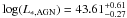 erg s-1
and
erg s-1
and  .
For the other redshifts, the L∗,AGN was kept constant and only
the normalisation constant was determined using all datapoints at a particular redshift.
This is based on the two assumptions that: i) the functional form of the AGN fraction is
similar at all redshifts; and ii) that the Lyα luminosity above which all
emitters are AGN does not change with redshift. These fits are also shown in the figure. A
clear evolution from higher to lower redshift appears to be present.
.
For the other redshifts, the L∗,AGN was kept constant and only
the normalisation constant was determined using all datapoints at a particular redshift.
This is based on the two assumptions that: i) the functional form of the AGN fraction is
similar at all redshifts; and ii) that the Lyα luminosity above which all
emitters are AGN does not change with redshift. These fits are also shown in the figure. A
clear evolution from higher to lower redshift appears to be present.
3. Evolution in the AGN fraction with time
To illustrate the evolution of the LAE AGN fraction with time, the fraction of AGN LAEs in the sample was extracted from the fits at three different Lyα luminosities, i.e. the AGN fraction that a given exponential fit in Fig. 1 gives for a certain Lyα luminosity, and plotted as a function of redshift in Fig. 2.
 |
Fig. 2 Evolution in AGN fraction above a given Lyα luminosity as a function of age of the Universe. Colour scheme is identical to Fig. 1 and refers to redshift. Different symbols mark the AGN fractions above three representative Lyα luminosities. The black lines are fits to the data, see text for explanation. A transition redshift at z ~ 2.5 (age ~ 2.5 Gyrs) is seen in all fits independent of luminosity limit. The purple line shows the redshift transition of the fraction of ULIRGs in LAE samples as presented in Nilsson & Møller (2009). |
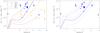 |
Fig. 3 LAE volume densities as a function of redshift and limiting Lyα luminosity. The datapoints are collected from 18 publications, searching for LAEs, with colour coding referring to the limiting Lyα luminosity in each survey (where [blue, yellow, red] have log Lyα [<42.25, 42.25 − 42.75, > 42.75] erg s-1). Models (see text) come from Bongiorno et al. (2007, B07) and Hopkins et al. (2007, H07). To the left, all measurements and the two models (with MB < −22.0) are shown to the different Lyα luminosity limits. To the right, only models and measurements to the faintest luminosity limits are shown, and instead the effect of varying the luminosity of the AGN is shown. For each model the grey lines show the predictions for MB < −20.0 (above the original line) or MB < −24.0 (below the original line). |
 (2)In this equation,
AF is the AGN fraction, θ represents the steepness of
the transition, and ztr is the transition redshift. The best-fit
values for the different Lyα luminosity limits can be found in Table 1. The most interesting parameter is the transition
redshift. It appears that the brightest AGN transition from lower to higher fractions first,
while fainter AGN remain less numerous until later times. This is consistent with a
down-sizing scenario, where the larger galaxies/AGN form first (Juneau et al. 2005). Comparing the results with those for the LAE
ULIRGs shows the transition for the ULIRGs to be sharper than those for the AGN, with a
transition redshift nearer to those of the brighter LAE AGN.
(2)In this equation,
AF is the AGN fraction, θ represents the steepness of
the transition, and ztr is the transition redshift. The best-fit
values for the different Lyα luminosity limits can be found in Table 1. The most interesting parameter is the transition
redshift. It appears that the brightest AGN transition from lower to higher fractions first,
while fainter AGN remain less numerous until later times. This is consistent with a
down-sizing scenario, where the larger galaxies/AGN form first (Juneau et al. 2005). Comparing the results with those for the LAE
ULIRGs shows the transition for the ULIRGs to be sharper than those for the AGN, with a
transition redshift nearer to those of the brighter LAE AGN.
4. Discussion
4.1. AGN and LAE volume density evolution
Having determined the AGN and ULIRG fractions among LAEs, one may ask the question of how these fractions relate to the general evolution of galaxy properties with redshift. An independent test of the determined AGN fraction is to calculate the LAE volume density by dividing a known AGN volume density by the LAE AGN fraction. For this test, we used the AGN comoving volume densities as determined observationally by Bongiorno et al. (2007) and theoretically by Hopkins et al. (2007), and we compared them with comoving LAE volume densities from eighteen different publications (Steidel et al. 2000; Stiavelli et al. 2001; Dawson et al. 2004; Hayashino et al. 2004; Shimasaku et al. 2006; Nilsson et al. 2007; Gronwall et al. 2007; Venemans et al. 2007; Murayama et al. 2007; Prescott et al. 2008; Deharveng et al. 2008; Ouchi et al. 2008; Nilsson et al. 2009; Grove et al. 2009; Shioya et al. 2009; Guaita et al. 2010; Bongiovanni et al. 2010; Yuma et al. 2010). In Fig. 3 these LAE volume densities are shown, together with the predictions. In the following, all type 1 AGN are assumed to have strong enough Lyα emission lines to be detected as LAEs. The predictions in the left panel are done for AGN brighter than MB < −22, as the z = 2.25 LAE AGN from Nilsson et al. (2009) are all brighter than this magnitude. Beyond z ~ 4.5, both models and measurements become uncertain. At z = 2 − 3 the measurements agree reasonably well with the expectations. The volume density at z = 0.3 is significantly too high, compared to the models. The scatter in the datapoints is large, probably owing to different selection criteria for the different surveys, but the overall trends are clear; the LAE volume density remains relatively flat over the redshift range z = 2−6, but falls at low redshift. The volume density of LAEs predicted by the AGN fraction, in turn, steeply increases towards higher redshift. In the range z = 2−3, the predictions and the measurements agree well, but there is an apparent lack/surplus of LAEs at high/low redshift. One explanation to this trend may be that the LAE AGN have different luminosities at different redshifts. In the right panel of Fig. 3 the effect of varying the AGN luminosity is shown. The volume density at z = 0.3 agrees better now, if all AGN at this redshift are very faint in the continuum. It becomes clear that the lack of LAEs at very high redshift (z > 4) can be explained if the AGN are all very luminous, and similarly that the surplus of AGN at z = 0.3 can be explained if all AGN are faint. The agreement between the LAE volume density and the predictions is an independent confirmation of the derived AGN fraction evolution, as well as an indication that the LAE AGN follow the general AGN evolutionary trends in the Universe.
4.2. Lyα emitters as tracers of galaxy evolution
The apparent trends displayed by LAEs as a function of redshift are easily explained with a simple, phenomenological model when considering which objects in the Universe emit Lyα photons. At high redshift (z > 3), most galaxies have low stellar masses and are in their first star forming episode. AGN and ULIRG number densities are low. Most Lyα photons at this time will thus trace this; young, small star-forming galaxies in their first starburst, with little dust content. Very few AGN or ULIRG LAEs will be found. A Gyr later, at z ~ 2, both the star formation rate density and the AGN number density are peaking. Some galaxies are already in their second, or even a later, starburst. Now the sample of Lyα-selected galaxies will reflect this diversity, with more AGN and ULIRG LAEs detected and a wider range of stellar properties (cf. Pentericci et al. 2009; Nilsson et al. 2011). Whereas there will be some galaxies in the same stage of evolution as at higher redshift, there will also be some galaxies with evolved stellar populations that are experiencing more recent star formation. These galaxies can be more massive and/or more dusty. The study of the redshift evolution of LAEs can thus be seen as an evolution in Lyα emission in the Universe, and could as such be an interesting test of galaxy evolution models including star formation, dust effects, and AGN number densities. In this model, no assumption about the evolution of individual LAEs is made. It is unlikely that LAEs at higher redshift will appear as such at lower redshift. The argument here is rather that LAEs are a random subset of all star-forming or active galaxies at a certain time, which happen to be in a Lyα emitting phase. Also, from this data it is not possible to draw any conclusions about the evolution of passive (i.e. non-star-forming or inactive) galaxies.
5. Conclusion
Based on the apparent evolution of the AGN and ULIRG fractions of LAEs, which are fractions that are expected to follow the evolution of star-forming and active galaxy populations throughout the Universe, some conclusions can be drawn regarding the general galaxy evolution scenario. From the evolutions of the fractions and volume densities in Figs. 2 and 3 it is seen that at first, in the very young (z > 4) Universe, only stars formed, regardless of AGN or ULIRGs. Later, at an age of approximately 3 Gyrs or redshift ~2.5, a secondary process started, suddenly increasing the number of both AGN and ULIRGs in the galaxy population. After this abrupt increase in dusty and active galaxies, an equilibrium was reached that has lasted to this day. A possible explanation for this very stable equilibrium may be the feed-back effects controlling the SFR in the galaxies. It is clear that this remains speculation until further data is collected, but proves the importance of studying objects emitting Lyα emission in the Universe.
Acknowledgments
The authors wish to thank Lucia Guaita for providing information about the AGN in CDFS, Yujin Yang for useful comments on the draft, and the anonymous referee for well-informed comments on the manuscript.
References
- Atek, H., Kunth, D., Schaerer, D., et al. 2009, A&A, 506, L1 [NASA ADS] [CrossRef] [EDP Sciences] [Google Scholar]
- Dawson, S., Rhoads, J. E., Malhotra, S., et al. 2004, ApJ, 617, 707 [NASA ADS] [CrossRef] [Google Scholar]
- Deharveng, J.-M., Small, T., Barlow, T. A., et al. 2008, ApJ, 680, 1072 [NASA ADS] [CrossRef] [Google Scholar]
- Dijkstra, M., Haiman, Z., & Spaans, M. 2006a, ApJ, 649, 14 [NASA ADS] [CrossRef] [Google Scholar]
- Dijkstra, M., Haiman, Z., & Spaans, M. 2006b, ApJ, 649, 37 [NASA ADS] [CrossRef] [Google Scholar]
- Elvis, M., Civano, F., Vignali, C., et al. 2009, ApJS, 184, 158 [NASA ADS] [CrossRef] [Google Scholar]
- Finkelstein, S. L., Rhoads, J. E., Malhotra, S., Pirzkal, N., & Wang, J. 2007, ApJ, 660, 1023 [NASA ADS] [CrossRef] [Google Scholar]
- Finkelstein, S. L., Cohen, S. H., Malhotra, S., Rhoads, J. E., & Papovich, C. 2009, ApJ, 703, L162 [NASA ADS] [CrossRef] [Google Scholar]
- Fynbo, J. P. U., Ledoux, C., Møller, P., Thomsen, B., & Burud, I. 2003, A&A, 407, 147 [NASA ADS] [CrossRef] [EDP Sciences] [Google Scholar]
- Gronwall, C., Ciardullo, R., Hickey, T., et al. 2007, ApJ, 667, 79 [NASA ADS] [CrossRef] [Google Scholar]
- Grove, L. F., Fynbo, J. P. U., Ledoux, C., et al. 2009, A&A, 497, 689 [NASA ADS] [CrossRef] [EDP Sciences] [Google Scholar]
- Guaita, L., Gawiser, E., Padilla, N., et al. 2010, ApJ, 714, 255 [NASA ADS] [CrossRef] [Google Scholar]
- Hasinger, G., Cappelluti, N., Brunner, H., et al. 2007, ApJS, 172, 29 [NASA ADS] [CrossRef] [Google Scholar]
- Hayashino, T., Matsuda, Y., Tamura, H., et al. 2004, AJ, 128, 2073 [NASA ADS] [CrossRef] [Google Scholar]
- Hibon, P., Cuby, J.-G., Willis, J., et al. 2010, A&A, 515, A97 [NASA ADS] [CrossRef] [EDP Sciences] [Google Scholar]
- Hogg, D. W., Cohen, J. G., Blandford, R., & Pahre, M. A. 1998, ApJ, 504, 622 [NASA ADS] [CrossRef] [Google Scholar]
- Hopkins, A. M. 2004, ApJ, 615, 209 [NASA ADS] [CrossRef] [Google Scholar]
- Hopkins, A. M., & Beacom, J. F. 2006, ApJ, 651, 142 [NASA ADS] [CrossRef] [MathSciNet] [Google Scholar]
- Hopkins, P. F., Richards, G. T., & Hernquist, L. 2007, ApJ, 654, 731 [NASA ADS] [CrossRef] [Google Scholar]
- Juneau, S., Glazebrook, K., Crampton, D., et al. 2005, ApJ, 619, L135 [NASA ADS] [CrossRef] [Google Scholar]
- Kauffmann, G., & Haehnhelt, M. 2000, MNRAS, 311, 576 [NASA ADS] [CrossRef] [Google Scholar]
- Miyaji, T., Hasinger, G., & Schmidt, M. 2000, A&A, 353, 25 [NASA ADS] [Google Scholar]
- Møller, P., & Warren, S. J. 1993, A&A, 270, 43 [NASA ADS] [CrossRef] [Google Scholar]
- Murayama, T., Taniguchi, Y., Scoville, N. Z., et al. 2007, ApJS, 172, 523 [NASA ADS] [CrossRef] [Google Scholar]
- Nilsson, K. K., & Møller, P. 2009, A&A, 508, L21 [NASA ADS] [CrossRef] [EDP Sciences] [Google Scholar]
- Nilsson, K. K., Fynbo, J. P. U., Møller, P., Sommer-Larsen, J., & Ledoux, C. 2006, A&A, 452, L23 [NASA ADS] [CrossRef] [EDP Sciences] [Google Scholar]
- Nilsson, K. K., Møller, P., Möller, O., et al. 2007, A&A, 471, 71 [NASA ADS] [CrossRef] [EDP Sciences] [Google Scholar]
- Nilsson, K. K., Tapken, C., Møller P., et al. 2009, A&A, 498, 13 [NASA ADS] [CrossRef] [EDP Sciences] [Google Scholar]
- Nilsson, K. K., Östlin, G., Møller, P., et al. 2011, A&A, submitted [arXiv:1009.0007] [Google Scholar]
- Ouchi, M., Shimasaku, K., Akiyama, M., et al. 2008, ApJS, 176, 301 [NASA ADS] [CrossRef] [Google Scholar]
- Pentericci, L., Grazian, A., Fontana, A., et al. 2009, A&A, 494, 553 [NASA ADS] [CrossRef] [EDP Sciences] [Google Scholar]
- Prescott, M. K. M., Kashikawa, N., Dey, A., & Matsuda, Y. 2008, ApJ, 678, L77 [NASA ADS] [CrossRef] [Google Scholar]
- Scarlata, C., Colbert, J., Teplitz, H. I., et al. 2009, ApJ, 704, L98 [NASA ADS] [CrossRef] [Google Scholar]
- Shimasaku, K., Kashikawa, N., Doi, M., et al. 2006, PASJ, 58, 313 [NASA ADS] [Google Scholar]
- Shinnerer, E., Smolcić, V., Carilli, C. L., et al. 2007, ApJS, 172, 46 [NASA ADS] [CrossRef] [Google Scholar]
- Shioya, Y., Taniguchi, Y., Sasaki, S. S., et al. 2009, ApJ, 696, 546 [NASA ADS] [CrossRef] [Google Scholar]
- Stiavelli, M., Scarlata, C., Panagia, N., et al. 2001, ApJ, 561, L37 [NASA ADS] [CrossRef] [Google Scholar]
- Steidel, C. C., Adelberger, K., Shapley, A. E., et al. 2000, ApJ, 532, 170 [Google Scholar]
- Venemans, B. P., Röttgering, H. J. A., Miley, G. K., et al. 2007, A&A, 461, 823 [NASA ADS] [CrossRef] [EDP Sciences] [Google Scholar]
- Wang, J. X., Rhoads, J. E., Malhotra, S., et al. 2004, ApJ, 608, 21 [Google Scholar]
- Wolf, C., Wisotzki, L., Borch, A., et al. 2003, A&A, 408, 499 [NASA ADS] [CrossRef] [EDP Sciences] [Google Scholar]
- Yuma, S., Ohta, K., Yabe, K., et al. 2010, ApJ, 720, 1016 [NASA ADS] [CrossRef] [Google Scholar]
All Tables
All Figures
|
Fig. 1 Cumulative fraction of non-AGN LAEs as a function of Lyα luminosity. Black dots are from the Nilsson et al. (2009) sample. Coloured points are from publications at redshifts z = 0.3 (Atek et al. 2009; Cowie et al. 2010; Finkelstein et al. 2009; Scarlata et al. 2009), z = 2.1 (Guaita et al. 2010), z = 3 (Gronwall et al. 2007; Ouchi et al. 2008) and at z ~ 4−5 (Wang et al. 2004; Ouchi et al. 2008). Lines indicate best-fit models (see text for details). |
| In the text | |
|
Fig. 2 Evolution in AGN fraction above a given Lyα luminosity as a function of age of the Universe. Colour scheme is identical to Fig. 1 and refers to redshift. Different symbols mark the AGN fractions above three representative Lyα luminosities. The black lines are fits to the data, see text for explanation. A transition redshift at z ~ 2.5 (age ~ 2.5 Gyrs) is seen in all fits independent of luminosity limit. The purple line shows the redshift transition of the fraction of ULIRGs in LAE samples as presented in Nilsson & Møller (2009). |
| In the text | |
|
Fig. 3 LAE volume densities as a function of redshift and limiting Lyα luminosity. The datapoints are collected from 18 publications, searching for LAEs, with colour coding referring to the limiting Lyα luminosity in each survey (where [blue, yellow, red] have log Lyα [<42.25, 42.25 − 42.75, > 42.75] erg s-1). Models (see text) come from Bongiorno et al. (2007, B07) and Hopkins et al. (2007, H07). To the left, all measurements and the two models (with MB < −22.0) are shown to the different Lyα luminosity limits. To the right, only models and measurements to the faintest luminosity limits are shown, and instead the effect of varying the luminosity of the AGN is shown. For each model the grey lines show the predictions for MB < −20.0 (above the original line) or MB < −24.0 (below the original line). |
| In the text | |
Current usage metrics show cumulative count of Article Views (full-text article views including HTML views, PDF and ePub downloads, according to the available data) and Abstracts Views on Vision4Press platform.
Data correspond to usage on the plateform after 2015. The current usage metrics is available 48-96 hours after online publication and is updated daily on week days.
Initial download of the metrics may take a while.