| Issue |
A&A
Volume 527, March 2011
|
|
|---|---|---|
| Article Number | A73 | |
| Number of page(s) | 10 | |
| Section | Planets and planetary systems | |
| DOI | https://doi.org/10.1051/0004-6361/201015579 | |
| Published online | 27 January 2011 | |
Gran Telescopio Canarias OSIRIS transiting exoplanet atmospheric survey: detection of potassium in XO-2b from narrowband spectrophotometry ⋆
1
Astrophysics Group, School of Physics, University of Exeter,
Stocker Road,
Exeter
EX4 4QL,
UK
e-mail: This email address is being protected from spambots. You need JavaScript enabled to view it.
2
Harvard-Smithsonian Center for Astrophysics, 60 Garden Street,
Cambridge,
MA
02138,
USA
3
Department of Astronomy and Astrophysics, University of
California, Santa
Cruz, CA
95064,
USA
4
Institut d’Astrophysique de Paris, UMR7095 CNRS, Université Pierre
& Marie Curie, 98bis
boulevard Arago, 75014
Paris,
France
5
Lunar and Planetary Laboratory, University of Arizona,
Sonett Space Science
Building, Tucson,
AZ
85721-0063,
USA
6
Departamento de Astrofísica, Universidad de La Laguna, Instituto
de Astrofísica de Canarias, La
Laguna, Tenerife,
Spain
7
Laboratoire d’Astrophysique de Grenoble, Université Joseph
Fourier, CNRS (UMR 5571), BP
53, 38041
Grenoble Cedex 9,
France
8
Carnegie Institution of Washington, Department of Terrestrial
Magnetism, 5241 Broad Branch Road
NW, Washington,
DC
20015,
USA
9
Institut de Ciencies de l’Espai (CSIC-ICE), Campus UAB, Facultat
de Ciencies, Torre C5, parell, 2a
pl, 08193 Bellaterra, Barcelona, Spain
Received:
13
August
2010
Accepted:
16
December
2010
Abstract
We present Gran Telescopio Canarias (GTC) optical transit narrowband photometry of the hot-Jupiter exoplanet XO-2b using the OSIRIS instrument. This unique instrument has the capabilities to deliver high-cadence narrowband photometric lightcurves, allowing us to probe the atmospheric composition of hot Jupiters from the ground. The observations were taken during three transit events that cover four wavelengths at spectral resolutions near 500, necessary for observing atmospheric features, and have near-photon limited sub-mmag precisions. Precision narrowband photometry on a large aperture telescope allows for atmospheric transmission spectral features to be observed for exoplanets around much fainter stars than those of the well studied targets HD 209458b and HD 189733b, providing access to the majority of known transiting planets. For XO-2b, we measure planet-to-star radius contrasts of Rpl/R⋆ = 0.10508 ± 0.00052 at 6792 Å, 0.10640 ± 0.00058 at 7582 Å, and 0.10686 ± 0.00060 at 7664.9 Å, and 0.10362 ± 0.00051 at 8839 Å. These measurements reveal significant spectral features at two wavelengths, with an absorption level of 0.067 ± 0.016% at 7664.9 Å caused by atmospheric potassium in the line core (a 4.1-σ significance level), and an absorption level of 0.058 ± 0.016% at 7582 Å, (a 3.6-σ significance level). When comparing our measurements to hot-Jupiter atmospheric models, we find good agreement with models that are dominated in the optical by alkali metals. This is the first evidence for potassium in an extrasolar planet, an element that has along with sodium long been supposed to be a dominant source of opacity at optical wavelengths for hot Jupiters.
Key words: planetary systems / stars: individual: XO-2 / techniques: photometric
Based on observations made with the Gran Telescopio Canarias (GTC), installed in the Spanish Observatorio del Roque de los Muchachos of the Instituto de Astrofísica de Canarias, in the island of La Palma, and part of the large ESO program 182.C-2018.
Hubble Fellow.
© ESO, 2011
1. Introduction
Transiting hot-Jupiter exoplanets provide an excellent opportunity to detect and characterize exoplanetary atmospheres. During a transit event, the opaque body of the planet and its atmosphere block light from the parent star, allowing the radius and its wavelength dependence to be accurately measured, which provide the means for the detection of atomic and molecular features in the atmosphere. In addition, secondary eclipse measurements can be used to obtain an exoplanet’s emission spectra, where such properties as the temperature, thermal structure, and composition can be measured (e.g. Deming et al. 2005; Grillmair et al. 2007; Charbonneau et al. 2008; Rogers et al. 2009; Sing & López-Morales 2009), while orbital phase curves can probe the global temperature distribution (Knutson et al. 2007).
For highly irradiated planets, the atmosphere at optical wavelengths represents the “window” into the planet where the bulk of the stellar flux is deposited. Thus, the atmospheric properties at these wavelengths are directly linked to important global properties such as atmospheric circulation, thermal inversion layers, and inflated planetary radii. All these features may be linked within the hot-Jupiter exoplanetary class (Fortney et al. 2008), and transmission spectra can provide direct observational constraints and fundamental measurements of the atmospheric properties at these crucial wavelengths. In the optical, hot-Jupiter transmission spectra are thought to be largely dominated by the opacity sources of the alkali metals sodium and potassium, with both species predicted to be present since the initial model calculations of highly irradiated gas giant exoplanets (Seager & Sasselov 2000; Brown 2001; Hubbard et al. 2001). Other strong but still unidentified optical absorbers could also play a role in the formation of stratospheres (Burrows et al. 2007; Knutson et al. 2008), with the leading candidates being TiO/VO and sulfur compounds (Hubeny et al. 2003; Fortney et al. 2008; Désert et al. 2008; Zahnle et al. 2009). No candidate is yet a clear favorite to universally produce hot-Jupiter stratospheres, both the TiO and sulfur explanations have unresolved issues (Spiegel et al. 2009) and stellar activity levels could also be important (Knutson et al. 2010).
To date, only two exoplanets have been ideal for optical atmospheric studies, HD 209458b and HD 189733b, mainly because of the stellar brightness (V ~ 7.8) and the large transit signals and low surface gravities. Atmospheric sodium has been detected in HD209458b from data with HST STIS (Charbonneau et al. 2002; Sing et al. 2008a,b) and confirmed by ground-based spectrographs (Snellen et al. 2008). In HD 189733b, a ground-based detection of sodium has also been made by Redfield et al. (2008), with the wider overall optical spectrum consistent with a high-altitude haze (Pont et al. 2008; Sing et al. 2009; Désert et al. 2009), which is thought to be caused by Rayleigh scattering by small condensate particles (Lecavelier des Etangs et al. 2008). While sodium has been detected in both planets, the other important alkali metal potassium has not, though in principle the ground-based as well as the HST spectra should have sufficient sensitivity.
Here we present the first results from GTC OSIRIS for the exoplanet XO-2b, which is part of our larger spectrophotometric optical survey of transiting hot Jupiters. XO-2b is a 0.996 RJup, 0.565 MJup planet in a 2.6 day orbital period around a non-active V = 11.2 early K dwarf star (Burke et al. 2007). XO-2b falls in the transition zone between the proposed “pM/pL” hot-Jupiter classification system of Fortney et al. (2008) and has been recently reported to perhaps have a “weak” thermal inversion layer (Machalek et al. 2009). Our overall program goals are to detect atmospheric features across a wide range of hot-Jupiter atmospheres, which will enable us to compare the observed features (comparative exoplanetology). OSIRIS is an optical imager and spectrograph on the new 10.4 m GranTeCan (GTC) telescope, capable of extremely high-precision differential narrowband fast photometry even for fainter transit hosting stars (Colón et al. 2010a). In our program, transit events are observed with a narrowband tunable filter, which is capable of simultaneously providing the spectral resolution and the extremely high photometric precision necessary to detect atmospheric transmission spectral features. Multiple wavelengths are chosen to be maximally sensitive to the expected hot-Jupiter atmospheric features, including sodium, potassium, and titanium oxide. An important advantage with spectrophotometry is that the absolute transit depths of each wavelength are measured, which allows us to compare atmospheric features with existing broadband data at other wavelengths. In addition, transit timing variation studies can also be made along with refining an exoplanet’s system parameters. We describe the GTC XO-2b observations in Sect. 2, present the analysis of the transit light curves in Sect. 3, discuss the results and compare them with model atmospheres in Sect. 4. We conclude in Sect. 5.
2. Observations
We observed with the GTC 10.4 m telescope installed in the Spanish Observatorio del Roque de los Muchachos of the Instituto de Astrofísica de Canarias on the island of La Palma, using the Optical System for Imaging and low Resolution Integrated Spectroscopy (OSIRIS) instrument during three separate nights in service mode.
2.1. GTC OSIRIS instrument setup
The GTC OSIRIS instrument (Cepa et al. 2000, 2003) consists of a mosaic of two Marconi CCD detectors, each with 2048 × 4096 pixels and a total field of view of 7.8 ′ × 8.5′, giving a plate scale of 0.127′′/pixel. The CCD has a pixel well depth of ~100 000 electrons and a 16 bit A/D converter, which saturates at 65 536 counts. For our observations we choose the 1 × 1 binning mode with a full frame readout at a speed of 500 kHz, which produces a readout overhead time of 31.15 s. The readout speed of 500 kHz has a gain of 1.46 e−/ADU and a readout noise of 8 e−. While 500 kHz is the noisiest readout speed (100 and 200 kHz are available), it allows for the most counts per image to be obtained owing to a higher gain. Our initial service mode observations were taken with the initially available full-frame readout mode, a conservative observing approach for our initial observations, with highly efficient windowing now becoming available. In future observations, windowing (sub-arrays) will eliminate nearly all CCD readout time and provide better time-sampling with a near 100% duty cycle.
We used the tunable filter (TF), which allows for narrowband imaging capable of specifying the wavelength(s) of our target and reference stars. The TF consists of a Fabry-Perot etalon, whose cavity separation can be adjusted, which provides a wide range of resolving powers, with OSIRIS capable of R = 300 to 1000. The unwanted orders from the etalon are then blocked by a set of broadband and mediumband (100–600 Å FWHM) filters. Different path-lengths through the optical system produce a wavelength dependance within the field of view in a way that each image has “rings” of constant wavelength with respect to the TF-center, located near the middle of the detector system (see Fig. 1). To provide a maximum spectral resolution and largest contrast for atmospheric signatures, we chose to observe with the narrowest width available to all wavelengths of 12 Å.
For the XO-2b observations we placed the target and a chosen nearby reference star, XO-2’s stellar companion XO-2B, at the same radial distance from the TF-center in a way that they would be observed at the same wavelength (see Fig. 1). The companions XO-2 and XO-2B are separated by 31″ and are cataloged to have the same spectral type (K0V) and very similar magnitudes and colors, which makes XO-2B an ideal reference star. When searching for the strong atmospheric potassium line, successive images were taken alternating between two different wavelength positions, which were carefully chosen to also avoid bright sky lines and strong telluric absorption lines, yet were located sufficiently close in wavelength to be within the same order-sorter filter. Because the tunable filter can scan very rapidly (~1 ms) and accurately (~0.1 Å) between wavelengths within a given order-sorter filter, we were able to observe at two potassium line wavelengths during a single transit while avoiding the typical long overheads associated with switching between traditional filters.
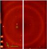 |
Fig. 1 GTC Osiris CCD frame of XO-2 on 4 December 2009 taken with the tunable filter, with CCD1 (left) and CCD2 (right). XO-2 is the circled bright star located near the center of CCD1, with XO-2’s stellar companion, used for our reference star, nearby and directly overhead. The z-scale of the image was set to best enhance the weak emission sky lines, which can be seen as “rings” around the image. Vignetting from components inside the instrument produced the artifacts at the very left edge of the image. |
2.2. Observing log
XO-2 was observed during the three transit events on 13 November 2009, 04 December 2009, and 03 March 2010 (see Table 1).
GTC OSIRIS XO-2 observations.
13 November 2009: The seeing was very good during the observations, with values ranging from 0.6″ to 0.9″. The filter was tuned to a single wavelength of 6792.0 Å, with 20.467 s exposure times used during the observing sequence with about 250 exposures acquired. There was an interruption of 20 min during the observations owing to problems with the M2 collimator, because of which we largely lost ingress. The out-of-transit baseline flux was also truncated compared with the other nights, because time was lost with the guiding setup and the TF which entered a forbidden range at the end of the night, where calibration becomes very unreliable. However, we found there was still ample time to accurately measure the baseline flux both before and after the transit, and the interruptions and delays did not limit our analysis. While we observed, the airmass decreased during the night from values of 1.678 to 1.08.
4 December 2009: XO-2 was observed at two TF wavelengths for the transit, and we switched successive images between 7664.89 and 7582 Å. The night was photometric, weather conditions very stable, and the seeing was very good during the sequence, with values ranging from 0.7″ to 0.9″. Approximately 150 exposures at each wavelength were acquired. The total exposure time was 25.466 s for each image, producing successive frames at the same wavelength every 113.2 seconds, and an overall duty cycle of 45%. During the observations the airmass decreased during the night from values of 2.158 to 1.081.
3 March 2010: Weather conditions were very stable, and the seeing was good during the sequence, with values ranging from 0.7″ to 0.9″. The filter was tuned to a single wavelength of 8839.0Å, with 40.67 s exposure times used during the observing sequence with about 230 exposures acquired. During the observations the airmass increased during the night from values of 1.078 to 1.639.
We did not modify the exposure times during the sequence in the three nights and maintained the peak counts around 30 000–35 000 ADUs for the reference and target stars. When needed, defocusing was used to avoid saturation in improved seeing conditions. No recalibration of the TF was needed during the observing sequences, because the field rotator moved in a range where no variations are expected. The data obtained during TF commissioning show that possible variations in the central wavelength of the TF in the present observations are smaller than 1 Å, with real variations likely even lower. In addition, the image monitoring every 10 min using strong sky lines showed no variation in TF tuning during the observations.
For each night 100 bias and 100 well exposed dome flat-field images were taken (~30 000 ADU/pixel/image). Our program uses dome-flats, as opposed to sky-flats, because small scale pixel-to-pixel variations are a potentially important source of noise, which requires a large number of well exposed flats to effectively remove it. The dome lights are not very homogeneous, in wavelength or spatially, which complicates the flat-fielding of large-scale features, and we added an illumination correction to the final co-added flat-field image. Our observations were all specified to occur at the same pixel location (no dithering) to help suppress flat-fielding errors, and the guiding each night kept the target’s location within a few pixels.
2.3. Reduction
The bias frames and flat fields were combined with standard IRAF routines and were used to correct each image before aperture photometry was performed with IDL for the target and reference stars. The aperture location was determined by fitting a 2D Moffat function (Moffat 1969) to the point spread function (PSF) of the target and reference stars within each image. The background sky was subtracted using the pixels from an annulus around each aperture. After selecting a wide range of apertures and sky annulus ring sizes, aperture radius sizes between 18 and 20 pixels were found to be optimal for our observations, along with sky annulus sizes in the ranges of 70 pixels for the inner sky ring radius and 150 pixels for outer radius. For a given night, the same sized apertures were used for the target and reference star. From our observed PSFs, the theoretical maximum S/N aperture (which balances the increased readout noise of including more pixels with the decreasing number of photons away from the PSF center, see Howell 2000) was found to be 20 pixels, in good agreement with the empirically determined optimal aperture size. For the December 2009 observations at 7582 Å, the average count level was observed to be 3.44 × 10⁶ counts for the target XO-2 and 3.55 × 10⁶ counts for the reference star XO-2B. Including the errors from photon-noise, readout noise, and sky subtraction, the average per-exposure uncertainty is found to be σXO2 = 0.00053 for XO-2 and σREF = 0.00053 for the reference star, giving a differential photometric lightcurve (LC) with an average per-exposure error of σLC = 0.00074, or a S/N per image of 1351. The error including photon, read noise, and sky background uncertainties were tabulated for each exposure and used as the estimate of the error in the differential photometric lightcurve. Similar values are found for the other two nights, with an average S/N per image of 1167 for the 6792 Å exposures and an average S/N of 1342 for the 8839 Å exposures.
The potassium line-core has nearby strong telluric O2 absorption lines, which could in principle affect the differential photometry. However, we found that the resulting atmospheric differential extinction between the target and reference star was negligible, <4 × 10⁻⁵, when modeling the transmission function t for each star through the atmosphere as a function of airmass, tsec(z) (Vidal-Madjar et al. 2010).
3. Analysis
3.1. Transit light curve fits
We modeled the transit light curve with the analytical transit models of Mandel & Agol (2002), fitting for the central
transit time, planet-to-star radius contrast, limb-darkening, inclination, stellar
density, and baseline flux. The errors on each datapoint were set to the tabulated values,
which included photon noise, sky subtraction, and readout noise. To account for the
effects of limb-darkening on the transit light curve, we adopted the three-parameter
limb-darkening law, 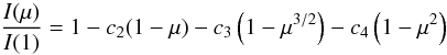 (1)and
calculated the coefficients following Sing (2010)
using the transmission through our narrowband tunable filters (see Table 2). We used the three-parameter non-linear
limb-darkening law, because it provides the best flexibility to capture the inherent
non-linearity of the limb-darkening intensity profile and helps to avoid the deficient
ATLAS model values near the limb (see Sing 2010,
for more details). This law has now successfully been used to model high precision transit
light curves including data from HST/NICMOS (Sing et al. 2009), Spitzer (Hébrard et al. 2010; Désert et al.
2011), and CoRot. In the fits we also allowed the baseline flux level of each
visit to linearly vary in time, which is described by the two fit-parameters. The linear
trend accounts for possible pixel-scale-related drifts during the observations, and we
found that two nights exhibited a small baseline gradient. The best-fit parameters were
determined simultaneously with a Levenberg-Marquardt least-squares algorithm (Markwardt 2009) using the unbinned data. A few deviant
points from each light curve were cut at the 3-σ level in the residuals,
which are likely caused by cosmic rays. The results from fitting each light curve
separately are given in Table 3. In the separate
light curve fits we allowed the linear coefficient term c2 to
vary freely, with the other two coefficients fixed to the predicted model values. Choosing
to fit only one limb-darkening parameter ensures that the fits are neither significantly
biased by adopting a stellar atmospheric model nor suffer from degeneracies between
fitting multiple limb-darkening parameters. The fit values for the linear limb-darkening
coefficients are measured at the ~4% level and are consistent
within 1σ of the model values (see Table 2), indicating that the Atlas models and three-parameters-law are
performing well.
(1)and
calculated the coefficients following Sing (2010)
using the transmission through our narrowband tunable filters (see Table 2). We used the three-parameter non-linear
limb-darkening law, because it provides the best flexibility to capture the inherent
non-linearity of the limb-darkening intensity profile and helps to avoid the deficient
ATLAS model values near the limb (see Sing 2010,
for more details). This law has now successfully been used to model high precision transit
light curves including data from HST/NICMOS (Sing et al. 2009), Spitzer (Hébrard et al. 2010; Désert et al.
2011), and CoRot. In the fits we also allowed the baseline flux level of each
visit to linearly vary in time, which is described by the two fit-parameters. The linear
trend accounts for possible pixel-scale-related drifts during the observations, and we
found that two nights exhibited a small baseline gradient. The best-fit parameters were
determined simultaneously with a Levenberg-Marquardt least-squares algorithm (Markwardt 2009) using the unbinned data. A few deviant
points from each light curve were cut at the 3-σ level in the residuals,
which are likely caused by cosmic rays. The results from fitting each light curve
separately are given in Table 3. In the separate
light curve fits we allowed the linear coefficient term c2 to
vary freely, with the other two coefficients fixed to the predicted model values. Choosing
to fit only one limb-darkening parameter ensures that the fits are neither significantly
biased by adopting a stellar atmospheric model nor suffer from degeneracies between
fitting multiple limb-darkening parameters. The fit values for the linear limb-darkening
coefficients are measured at the ~4% level and are consistent
within 1σ of the model values (see Table 2), indicating that the Atlas models and three-parameters-law are
performing well.
We also performed a joint fit for the four light curves, simultaneously fitting for the
inclination i and stellar density
ρ⋆, with the limb-darkening values
fixed to the predicted model values. The results are plotted in Fig. 2. Because the precision and spectral resolution in our lightcurves are
sufficient to observe atmospheric features, which cause measurable changes in the planet’s
radii, we jointly fitted each light curve with a common reference planetary radius,
Rref = Rpl/R⋆
and with an altitude in units of stellar radius,
Z = Z(λ), above the fit reference
radius value with  (2)The transit light curve
at 8839 Å was used as the reference radius value, and we set the altitude
Z(8839) = 0 because it contained the smallest measured radius. The main
advantage of jointly fitting Rref for the different color
light curves and separately fitting Z(λ) is that the
uncertainties in fitting for the system parameters (i,
a/R⋆,
b, & ρ⋆) do not
affect the measurement (joint probability distribution) of
Z(λ), given that the correlations between the system
parameters and radius are largely wavelength-independent. We also quote the individual
Rpl/R⋆
values for each light curve when the system parameters are set to their best-fit values.
The results of these joint fits are given in Table 4.
(2)The transit light curve
at 8839 Å was used as the reference radius value, and we set the altitude
Z(8839) = 0 because it contained the smallest measured radius. The main
advantage of jointly fitting Rref for the different color
light curves and separately fitting Z(λ) is that the
uncertainties in fitting for the system parameters (i,
a/R⋆,
b, & ρ⋆) do not
affect the measurement (joint probability distribution) of
Z(λ), given that the correlations between the system
parameters and radius are largely wavelength-independent. We also quote the individual
Rpl/R⋆
values for each light curve when the system parameters are set to their best-fit values.
The results of these joint fits are given in Table 4.
Three-parameter non-linear limb darkening coefficients for GTC OSIRIS tunable filters.
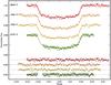 |
Fig. 2 GTC OSIRIS narrowband transit light curves at (top-to-bottom) 8839, 7665, 7582, and 6792 Å, with an arbitrary flux offset applied to each curve for clarity. The best-fit models are also over-plotted, along with the residuals (bottom four curves), which have a y-axis error bar corresponding to the per-point flux uncertainty. The light curves are near-Poisson limited, with per-point S/N levels between 1149 and 1351. |
System parameters for XO-2b from individual light curve fits.
3.2. Noise estimate
Each of our light curves achieves sub-mmag precision, with the RMS of the residuals between the best-fitting individual models and the data being 0.087% at 6792 Å (S/N of 1149), 0.074% at 7582 Å (S/N of 1351), 0.076% at 7664 Å (S/N of 1315), and 0.083% at 8839 Å (S/N of 1204). These values compare very favorably to the theoretically estimated error in Sect. 2, which is dominated by photon noise, which indicates that our transit light curves are regularly achieving between 90% to 100% of the theoretical Poisson limit, without having to use de-correlation techniques to remove systematic errors. Other sources of noise are found to be negligible. This includes scintillation, which was also found for the large aperture of GTC by Colón et al. (2010a).
We checked for the presence of systematic errors correlated in time (“red noise”, Pont et al. 2006) by checking that the binned residuals
followed a N −1/2 relation when binning in time by N
points. If there is red noise, the variance can be well modeled to follow a
 relation,
where σw is the uncorrelated white noise
component, while σr characterizes the red
noise. We found no significant evidence for red noise when binning on timescales up to the
ingress and egress duration with all determined
σr values below 1 × 10⁻⁴, a
level corresponding to the limiting precision that our radius values can be measured
within an individual light curve
(σR2 ~ 1.1 × 10⁻⁴).
When possible, we also checked for red noise with the wavelet-based method of Carter & Winn (2009) and found generally a good
agreement with the binning technique.
relation,
where σw is the uncorrelated white noise
component, while σr characterizes the red
noise. We found no significant evidence for red noise when binning on timescales up to the
ingress and egress duration with all determined
σr values below 1 × 10⁻⁴, a
level corresponding to the limiting precision that our radius values can be measured
within an individual light curve
(σR2 ~ 1.1 × 10⁻⁴).
When possible, we also checked for red noise with the wavelet-based method of Carter & Winn (2009) and found generally a good
agreement with the binning technique.
4. Discussion
The system parameters determined with the GTC light curves agree well (at the ~1-σ level) with the most accurate values for XO-2b previously published, namely the z-band measurements from Fernandez et al. (2009). We chose our wavelengths to be maximally sensitive to the potassium line, with the transits measured at 7664 and 7582 intended to measure the K I line core, while those at 6792 and 8834 Å were chosen to have minimum contributive opacities from K, Na, and H2O. Our joint-fit system parameters measure a significant altitude z at two wavelengths, with the measured potassium line center at 7664 Å to be z(7664) = 0.00322 ± 0.00079 R⋆, which is above the reference altitude at the 4.1-σ significance level (“absorption” level of Δ(Rpl/R⋆)2 = 0.067 ± 0.016%). Assuming the stellar radius as given in Table 4, the potassium line core is seen to reach altitudes of 2190 ± 540 km above the 8839 Å reference planetary radius. A significant altitude is also measured at 7582 Å, with z(7582) = 0.00278 ± 0.00077 R⋆, which is above the reference zero altitude at the 3.6-σ significance level.
Joint-fit system parameters for XO-2b.
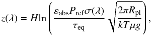 (3)where
εabs is the abundance of dominating absorbing species,
Pref is the pressure at the reference altitude,
σ(λ) is the absorption cross section,
and H is the atmospheric scale height. The measured altitude
parameter Z(λ) from Sect. 3 relates to
z(λ) by
Z(λ) = z(λ)/R⋆.
(3)where
εabs is the abundance of dominating absorbing species,
Pref is the pressure at the reference altitude,
σ(λ) is the absorption cross section,
and H is the atmospheric scale height. The measured altitude
parameter Z(λ) from Sect. 3 relates to
z(λ) by
Z(λ) = z(λ)/R⋆.
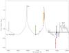 |
Fig. 3 XO-2b narrowband GTC photometric results at four wavelengths (colored points) along with the z-band radius (black dot) of Fernandez et al. (2009). The X-axis error bars indicate the wavelength range of the photometry, while the Y-axis error bars indicates the errors on the measured planetary radius, assuming a stellar radius of 0.976 R⊙. Also over-plotted is a 1500 K isothermal model (binned to R = 500) of the transmission spectrum from Fortney et al. (2010) adapted for XO-2b, which is dominated by gaseous Na and K. TiO and VO opacities are removed in this model. The open circles indicate the predicted filter-integrated model values. |
Assuming a temperature of 1500 K for XO-2 based on the broadband secondary eclipse measurements of Machalek et al. (2009) and a surface gravity of 14.71 m/s2 based on the planetary mass and radius values found by Fernandez et al. (2009), we estimate an atmospheric scale height of H = 370 km, and H/R⋆ = 0.00054. Thus, the individual precisions of our wavelength-dependent planetary radius measurements (σRpl/R⋆ ~ 0.00055 & σZ ~ 0.00075) correspond to one atmospheric scale height. The atmospheric feature at 7664 Å thus spans 6 ± 1.5 scale heights above the reference altitude.
4.1. Atmospheric signatures of potassium
We compare our best-fit planetary radius values to the recent hot-Jupiter model atmospheric calculations of Fortney et al. (2010), along with XO-2b specifically generated models. These models include a self-consistent treatment of radiative transfer and chemical equilibrium of neutral species, though they do not include the formation of hazes. Given our limited wavelength coverage, these physically motivated models are necessary for a comparison with our data, because there are not enough data to justify freely fitting for a large number of atmospheric parameters. The comparisons here are an effort to more broadly distinguish XO-2b’s atmosphere in different classes of models, given there are no prior constraints on the basic composition or presence of clouds/hazes, and to also compare the specific predictions that these models have for XO-2b.
The transmission spectrum calculations are performed for 1D atmospheric pressure-temperature (P-T) profiles. The model atmospheres use the equilibrium chemical abundances at solar metallicity described in Lodders & Fegley (2002, 2006). The opacity database is described in Freedman et al. (2008). The model atmosphere code has been used to generate P-T profiles for a variety of close-in planets (Fortney et al. 2005, 2006, 2008). The transmission spectrum calculations are described in Fortney et al. (2010). For XO-2b, we find that the optical opacity is dominated by gaseous Na and K, as is expected for many close-in planets over a broad temperature range (e.g., Sudarsky et al. 2000; Seager & Sasselov 2000). These alkalis may be subjected to photo-ionization, but this is not included in this study.
The models are calculated wavelength by wavelength at a resolution of R = 3500, which is about seven times higher than the resolution of our data. For the comparisons with the GTC data we assumed a value of R⋆ = 0.976 M⊙ (Table 3) and calculated the filter-integrated predictions from the high-resolution model, fitting only for an arbitrary model altitude shift. Our GTC measurements are well matched with theoretical models, which include significant opacity from atmospheric potassium. This is the first indications to date that this species is present in hot-Jupiter atmospheres.
Isothermal models: comparing the observed atmospheric features to isothermal hydrostatic uniform abundance models helps provide an overall understanding of the observed features and departures from those conditions. Using Eq. (3), we adapted generic hot-Jupiter isothermal models to values appropriate for XO-2. We find an isothermal model dominated by alkali metals in the optical is a substantially better fit than a gray “flat” atmosphere, as would be expected if high-altitude clouds were dominant. Adjusting only the model reference altitude (i.e. the model normalization) in the fits to the GTC and z-band points gives a χ2 of 22 with 4 degrees of freedom (DOF) for a gray featureless atmosphere and a χ2 of 7.0 for a 1500 K isothermal alkali-dominated atmosphere (see Fig. 3, with the model binned to R = 500). With a smaller scale height, a cooler 1000 K isothermal model somewhat under-predicts the K I core levels, producing a χ2 fit of 9.3 with 4 DOF.
Models including TiO and VO in addition to K I do not improve the fits. A 1500 K isothermal model including TiO and VO opacity at chemical equilibrium abundances gives a χ2 fit of 12.6 with 4 DOF (see Fig. 4). In these models, TiO/VO effectively raise the altitudes of the non-potassium core model levels, which degrades the fit. These models still predict the 7664 Å feature as caused by potassium, because the low levels of TiO do not cover the potassium core signature, with the K-doublet still visible in Fig. 4. Models completely dominated by only TiO/VO absorption, which is perhaps appropriate to very hot-Jupiters such as Wasp-12, can be definitively ruled out, because they provide a substantially poorer fit to the data (χ2 of 32). Sulfur compounds are unlikely to contribute at these longer wavelengths.
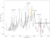 |
Fig. 4 Same as Fig. 3, but over-plotted with a 1500 K isothermal model also containing TiO/VO opacity, producing many strong absorption features. The TiO/VO abundances in the model are from equilibrium chemistry. There is no evidence for TiO/VO in the GTC data, because the model fits with TiO/VO are significantly worse than the alkali-dominated models (see text). |
XO-2b specific models: We also compared our GTC planetary radius values to models specifically calculated for the known parameters of XO-2b, assuming chemical equilibrium at solar metallicity. A model using a dayside-averaged temperature-pressure (T-P) profile (see Figs. 5 and. 6) is our best fitting model, giving a χ2 value of 6.6 for 4 DOF. The cooler model transmission spectra using a planet-wide averaged T-P profile (see Fig. 5), perform moderately worse, giving a fit with a χ2 of 8.0 for 4 DOF. The planet-wide averaged model predicts lower overall temperatures than the dayside model and also results in a slight under-prediction of the potassium line-core signature similar the 1000 K isothermal model.
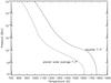 |
Fig. 5 Temperature-pressure profiles for the XO-2b specific models, including a planet-wide averaged profile (left) and a dayside-averaged profile (right). The GTC transit data are sensitive to pressures from ~10-1 bar at the lowest altitudes to ~10-3 bar at the highest altitudes in the potassium and sodium line-cores. |
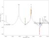 |
Fig. 6 Same as Fig. 3, but over-plotted with a XO-2b specific model of the transmission spectrum, which uses a dayside-averaged temperature-pressure profile. The model is dominated in the optical by Na and K absorption signatures. Compared with the isothermal model of Fig. 3, the lower temperatures at higher-altitudes in this model lead to a better fit of the K-core 7664.9 Å measurement. Additional observations are planned at blue wavelengths (blue boxes), which will be highly sensitive to atmospheric sodium, and will help provide a more complete picture of the transmission spectrum. |
4.2. Limits on stellar activity
A transmission spectrum in active stars can be affected by stellar spots when a spot is occulted by the planet and also by non-occulted spots during the epoch of the transit observations (Pont et al. 2008; Agol et al. 2010). A non-occulted stellar spot changes the baseline stellar flux with which the transit is normalized in a way that different epochs with different amounts of spots will show small but non-negligible radius changes. For the XO-2b observations, sufficiently strong stellar activity could in principle affect the measured radii at the reference wavelengths (6792 and 8839 Å) compared with the potassium line core wavelengths, because they were not taken simultaneously during a transit event. However, without strong stellar activity, multiple transits spanning long epochs (i.e. non-simultaneous transits) can still be used and fitted together at high precision, without the need for a stellar-activity-related correction.
Czesla et al. (2009) and Désert et al. (2011) proposed that the impact of rotation-modulated
spots on the final fitted radius could be estimated following
 (4)where fλ
is the relative variation of the stellar flux owing to stellar activity (i.e.
rotation-modulated spots) and α is an empirically determined constant on
the order of unity. On the hypothesis that the stellar surface brightness outside dark
stellar spots are not modified by the activity level, the parameter α is
given by −1. The range of fλ between active
and non-active stars is very large, spanning many orders of magnitude. For the highly
active star HD 189733, fλ ~ 2−3%
in the visible (Henry & Winn 2008), while
for the non-active star TrES-2, fλ was found
to have an amazingly low value of (5.18 ± 0.19) × 10-6 from the Kepler data
(Kipping & Bakos 2010). Ciardi et al. (2010) studied the stellar photometric
variability for stars in the Kepler sample, finding a bi-model distribution between active
and non-active stars. K-dwarfs with a low activity (2/3 of the sample) were found to
typically display a stochastic photometric variability of less than 1 mmag, while active
stars were often found to be periodic on timescales of days to weeks. For the HST transit
observations of the highly active star HD 189733 (Pont
et al. 2008; Sing et al. 2009; Désert et al. 2011), an observational strategy was
adopted to counter this effect, which involved monitoring the stellar activity level. In
this way, the stellar baseline flux was known at every epoch of the transit observations
and could then be used to correctly normalize the data. For non-active stars such as
TrES-2 or XO-2, this strategy may not be needed because the transit-fit planetary radii
values will not significantly change from one epoch to another.
(4)where fλ
is the relative variation of the stellar flux owing to stellar activity (i.e.
rotation-modulated spots) and α is an empirically determined constant on
the order of unity. On the hypothesis that the stellar surface brightness outside dark
stellar spots are not modified by the activity level, the parameter α is
given by −1. The range of fλ between active
and non-active stars is very large, spanning many orders of magnitude. For the highly
active star HD 189733, fλ ~ 2−3%
in the visible (Henry & Winn 2008), while
for the non-active star TrES-2, fλ was found
to have an amazingly low value of (5.18 ± 0.19) × 10-6 from the Kepler data
(Kipping & Bakos 2010). Ciardi et al. (2010) studied the stellar photometric
variability for stars in the Kepler sample, finding a bi-model distribution between active
and non-active stars. K-dwarfs with a low activity (2/3 of the sample) were found to
typically display a stochastic photometric variability of less than 1 mmag, while active
stars were often found to be periodic on timescales of days to weeks. For the HST transit
observations of the highly active star HD 189733 (Pont
et al. 2008; Sing et al. 2009; Désert et al. 2011), an observational strategy was
adopted to counter this effect, which involved monitoring the stellar activity level. In
this way, the stellar baseline flux was known at every epoch of the transit observations
and could then be used to correctly normalize the data. For non-active stars such as
TrES-2 or XO-2, this strategy may not be needed because the transit-fit planetary radii
values will not significantly change from one epoch to another.
With the TrES-2b Kepler data and this low level of activity, eighteen optical transits
were fitted together by Kipping & Bakos
(2010), who found no signs of epoch-dependent radius changes, which would be
apparent from strong activity-related effects. The star TrES-2 has very similar activity
indices to XO-2, with Knutson et al. (2010)
measuring the stellar activity indices of the Ca II H & K line strength to be
log ( ) = − 4.988 for
XO-2 and − 4.949 for TrES-2, while the S-value of XO-2 is 0.173 and 0.165 for TrES-2.
Similar activity levels as those of TrES-2 suggest that activity-related radius changes in
XO-2 are also negligible. The final TrES-2 combined transit light curve was successfully
fitted down to the 20 ppm level, which is nearly one order of magnitude below our required
levels for XO-2b (~100 ppm). Hat-P7 and Kepler-#4, #5, #6, #7, and #8 also show
a low photometric variability around the ~0.2 mmag level with removed transits
when calculating the light curve statistics (Ciardi et al.
2010), and all have similar activity indices to XO-2 (Knutson et al. 2010).
) = − 4.988 for
XO-2 and − 4.949 for TrES-2, while the S-value of XO-2 is 0.173 and 0.165 for TrES-2.
Similar activity levels as those of TrES-2 suggest that activity-related radius changes in
XO-2 are also negligible. The final TrES-2 combined transit light curve was successfully
fitted down to the 20 ppm level, which is nearly one order of magnitude below our required
levels for XO-2b (~100 ppm). Hat-P7 and Kepler-#4, #5, #6, #7, and #8 also show
a low photometric variability around the ~0.2 mmag level with removed transits
when calculating the light curve statistics (Ciardi et al.
2010), and all have similar activity indices to XO-2 (Knutson et al. 2010).
For XO-2 there is also no obvious evidence for occulted spots in any of our sub-mmag precision light curves, which is consistent with a non-active star, though non-occulted spot features could be clustered at different latitudes. In addition, no spot-induced rotational modulations have yet been reported, with the discovery XO-2 lightcurves seemingly constant down to a noise-limited ~7 mmag level (Burke et al. 2007). Assuming fλ < 0.007 for XO-2 and α = −1, we find Δ(Rpl/R⋆) < 0.00036, which is below the limiting precision level of our measurements and below the estimated size of one atmospheric scale height. While current evidence points toward XO-2 as being a non-active star with a likely small photometric variability, additional activity monitoring of this and other transit hosting stars can play an important role in assessing the true variability.
4.3. Transit timing studies
We used the four central transit times of our GTC data and the transit times of Burke et al. (2007) and Fernandez et al. (2009) to determine the transit ephemeris, using a linear
function of the period P and transit epoch E,
 (5)The results are given in
Table 4, where we find a period of
P = 2.61586178 ± 0.00000075 (days) and a mid-transit time of
T(0) = 2454466.88457 ± 0.00014 (HJD). A fit with a linear ephemeris is
in general an unsatisfactory fit to the data, because it has a
χ2 of 42 for 20 degrees of freedom
(
(5)The results are given in
Table 4, where we find a period of
P = 2.61586178 ± 0.00000075 (days) and a mid-transit time of
T(0) = 2454466.88457 ± 0.00014 (HJD). A fit with a linear ephemeris is
in general an unsatisfactory fit to the data, because it has a
χ2 of 42 for 20 degrees of freedom
( ). The
fit period is within 1-σ of the Burke
et al. (2007) value of 2.615857 ± 0.000005 days, but 3-σ away
from the period of 2.615819 ± 0.000014 days Fernandez
et al. (2009) found when fitting for the ephemeris with just their six transit
times. Similar to the conclusions of Fernandez et al.
(2009) we find that it is not clear whether to interpret the poor linear fit and
differences in period to a genuine period variation caused by a second planet, or if the
uncertainties in all the timings are underestimated by
). The
fit period is within 1-σ of the Burke
et al. (2007) value of 2.615857 ± 0.000005 days, but 3-σ away
from the period of 2.615819 ± 0.000014 days Fernandez
et al. (2009) found when fitting for the ephemeris with just their six transit
times. Similar to the conclusions of Fernandez et al.
(2009) we find that it is not clear whether to interpret the poor linear fit and
differences in period to a genuine period variation caused by a second planet, or if the
uncertainties in all the timings are underestimated by
 .
Given that the observed variations are so close to the per-transit noise level, an
unambiguous transit-timing variation and detection of a second planet free of systematic
errors will require more observations with generally improved timing errors. GTC OSIRIS
observations in sub-array mode should help provide the necessary precision, because the
duty cycle can be increased to near 100%.
.
Given that the observed variations are so close to the per-transit noise level, an
unambiguous transit-timing variation and detection of a second planet free of systematic
errors will require more observations with generally improved timing errors. GTC OSIRIS
observations in sub-array mode should help provide the necessary precision, because the
duty cycle can be increased to near 100%.
5. Conclusions
We presented GTC OSIRIS observations for three transits of XO-2b at four carefully selected narrowband wavelengths, which have revealed significant absorption by atmospheric potassium. This is the first evidence for this important alkali metal in an extrasolar planet, which has long been assumed to be a dominant source of opacity at optical wavelengths along with sodium. The identification of atmospheric contents is one of the first steps for understanding the nature of exoplanetary atmospheres. The presence (or lack) of key species can give clues on the exoplanet’s temperature, presence of condensate clouds, and chemistry and can potentially be used to assign different atmospheres and place exoplanets to different sub-classes. Clear gaseous hot-Jupiter atmospheres are thought to have low geometric albedos, appearing very dark at visible wavelengths, with broad pressure broadened potassium and sodium line-wings efficiently absorbing the incoming stellar radiation (Sudarsky et al. 2000; Seager et al. 2000). A detection of potassium in XO-2b helps support this overall picture. Potassium and sodium could also play important roles in inflating hot Jupiters through ohmic dissipation mechanisms (Batygin & Stevenson 2010). Notably, there is also no particular evidence for K I photoionization, which could have been evident by depletion at high altitudes.
Narrowband spectrophotometry is a robust method for obtaining precision differential photometric transit lightcurves, which have a spectral resolution sufficient to detect atmospheric transmission spectral features. OSIRIS is the first instrument capable of producing sub-mmag high-speed spectrophotometry, and coupled with the large 10.4 m aperture of GTC, is capable of detecting spectral features in transmission spectra on exoplanets such as XO-2b, whose host star is 3.5 mag fainter in the optical than those of the well studied transiting hot Jupiters HD 189733b and HD 209458b. XO-2b now joins those two exoplanets as the only hot-Jupiters where direct constraints on the atmospheric opacity in the optical can be made. Detecting and studying the atmospheres for these fainter targets will be critical for a broader understanding of the hot-Jupiter class as a whole, because most of the known transiting planets have been found at magnitudes >10. Further observations from our program, which will include planned XO-2b measurements at blue wavelengths, can help conclude whether the optical atmospheres of these exoplanets are dominated by the two alkali metals sodium and potassium together, search for Rayleigh scattering, and place limits on other optical absorbers that are thought to be linked to thermal inversion layers.
. Shortly before submission, we became aware of independent, but similar observations of another exoplanet (Colon et al. 2010b). Future observations of these and additional exoplanets will enable comparisons of the atmospheric composition and structure, as well as studies of potential correlations with other planet or host star properties.
Acknowledgments
We thank the entire GTC staff and especially Antonio Cabrera Lavers for his continued excellent work in executing this program. D.K.S. is pleased to note that part of this work was performed while in residence at the Kavli Institute for Theoretical Physics, funded by the NSF through grant No. PHY05-51164. This work was partially supported by the Spanish Plan Nacional de Astronomía y Astrofísica under grant AYA2008-06311-C02-01. D.E. is supported by the Centre National d’Études Spatiales (CNES). M.L.M. acknowledges support from NASA through Hubble Fellowship grant HF-01210.01-A/HF-51233.01 awarded by the STScI, which is operated by the AURA, Inc. for NASA, under contract NAS5-26555.
References
- Agol, E., Cowan, N. B., Knutson, H. A., et al. 2010, ApJ, 721, 1861 [NASA ADS] [CrossRef] [Google Scholar]
- Batygin, K. & Stevenson, D. J. 2010, ApJ, 714, L238 [NASA ADS] [CrossRef] [Google Scholar]
- Brown, T. M. 2001, ApJ, 553, 1006 [NASA ADS] [CrossRef] [Google Scholar]
- Burke, C. J., McCullough, P. R., Valenti, J. A., et al. 2007, ApJ, 671, 2115 [NASA ADS] [CrossRef] [Google Scholar]
- Burrows, A., Hubeny, I., Budaj, J., Knutson, H. A., & Charbonneau, D. 2007, ApJ, 668, L171 [NASA ADS] [CrossRef] [MathSciNet] [Google Scholar]
- Carter, J. A., & Winn, J. N. 2009, ApJ, 704, 51 [NASA ADS] [CrossRef] [Google Scholar]
- Cepa, J., Aguiar, M., Escalera, V. G., et al. 2000, in SPIE Conf. Ser. 4008, ed. M. Iye, & A. F. Moorwood, 623 [Google Scholar]
- Cepa, J., Aguiar-Gonzalez, M., Bland-Hawthorn, J., et al. 2003, in SPIE Conf. Ser. 4841, ed. M. Iye, & A. F. M. Moorwood, 1739 [Google Scholar]
- Charbonneau, D., Brown, T. M., Noyes, R. W., & Gilliland, R. L. 2002, ApJ, 568, 377 [NASA ADS] [CrossRef] [Google Scholar]
- Charbonneau, D., Knutson, H. A., Barman, T., et al. 2008, ApJ, 686, 1341 [NASA ADS] [CrossRef] [MathSciNet] [Google Scholar]
- Ciardi, D. R., von Braun, K., Bryden, G., et al. 2010 [arXiv:1009.1840] [Google Scholar]
- Colón, K. D., Ford, E. B., Lee, B., Mahadevan, S., & Blake, C. H. 2010a, MNRAS, 408, 1494 [NASA ADS] [CrossRef] [Google Scholar]
- Colon, K. D., Ford, E. B., Redfield, S., et al. 2010b [arXiv:1008.4800] [Google Scholar]
- Czesla, S., Huber, K. F., Wolter, U., Schröter, S., & Schmitt, J. H. M. M. 2009, A&A, 505, 1277 [NASA ADS] [CrossRef] [EDP Sciences] [Google Scholar]
- Deming, D., Seager, S., Richardson, L. J., & Harrington, J. 2005, Nature, 434, 740 [NASA ADS] [CrossRef] [PubMed] [Google Scholar]
- Désert, J.-M., Vidal-Madjar, A., Lecavelier des Etangs, A., et al. 2008, A&A, 492, 585 [NASA ADS] [CrossRef] [EDP Sciences] [Google Scholar]
- Désert, J.-M., Lecavelier des Etangs, A., Hébrard, G., et al. 2009, ApJ, 699, 478 [NASA ADS] [CrossRef] [Google Scholar]
- Désert, J., Sing, D., Vidal-Madjar, A., et al. 2011, A&A, 526, A12 [NASA ADS] [CrossRef] [EDP Sciences] [Google Scholar]
- Fernandez, J. M., Holman, M. J., Winn, J. N., et al. 2009, AJ, 137, 4911 [NASA ADS] [CrossRef] [Google Scholar]
- Fortney, J. J., Marley, M. S., Lodders, K., Saumon, D., & Freedman, R. 2005, ApJ, 627, L69 [NASA ADS] [CrossRef] [Google Scholar]
- Fortney, J. J., Saumon, D., Marley, M. S., Lodders, K., & Freedman, R. S. 2006, ApJ, 642, 495 [NASA ADS] [CrossRef] [Google Scholar]
- Fortney, J. J., Lodders, K., Marley, M. S., & Freedman, R. S. 2008, ApJ, 678, 1419 [NASA ADS] [CrossRef] [Google Scholar]
- Fortney, J. J., Shabram, M., Showman, A. P., et al. 2010, ApJ, 709, 1396 [NASA ADS] [CrossRef] [Google Scholar]
- Freedman, R. S., Marley, M. S., & Lodders, K. 2008, ApJS, 174, 504 [NASA ADS] [CrossRef] [Google Scholar]
- Grillmair, C. J., Charbonneau, D., Burrows, A., et al. 2007, ApJ, 658, L115 [NASA ADS] [CrossRef] [Google Scholar]
- Hébrard, G., Désert, J., Díaz, R. F., et al. 2010, A&A, 516, A95 [NASA ADS] [CrossRef] [EDP Sciences] [Google Scholar]
- Henry, G. W. & Winn, J. N. 2008, AJ, 135, 68 [NASA ADS] [CrossRef] [Google Scholar]
- Howell, S. B. 2000, Handbook of CCD Astronomy (Cambridge University Press) [Google Scholar]
- Hubbard, W. B., Fortney, J. J., Lunine, J. I., et al. 2001, ApJ, 560, 413 [NASA ADS] [CrossRef] [Google Scholar]
- Hubeny, I., Burrows, A., & Sudarsky, D. 2003, ApJ, 594, 1011 [NASA ADS] [CrossRef] [Google Scholar]
- Kipping, D. M., & Bakos, G. Á. 2010 [arXiv:1006.5680] [Google Scholar]
- Knutson, H. A., Charbonneau, D., Allen, L. E., et al. 2007, Nature, 447, 183 [NASA ADS] [CrossRef] [PubMed] [Google Scholar]
- Knutson, H. A., Charbonneau, D., Allen, L. E., Burrows, A., & Megeath, S. T. 2008, ApJ, 673, 526 [NASA ADS] [CrossRef] [Google Scholar]
- Knutson, H. A., Howard, A. W., & Isaacson, H. 2010, ApJ, 720, 1569 [NASA ADS] [CrossRef] [Google Scholar]
- Lecavelier des Etangs, A., Pont, F., Vidal-Madjar, A., & Sing, D. 2008, A&A, 481, L83 [NASA ADS] [CrossRef] [Google Scholar]
- Lodders, K., & Fegley, B. 2002, Icarus, 155, 393 [NASA ADS] [CrossRef] [Google Scholar]
- Lodders, K., & Fegley, Jr., B. 2006, Chemistry of Low Mass Substellar Objects, ed. Mason, J. W. (Springer Verlag), 1 [Google Scholar]
- Machalek, P., McCullough, P. R., Burrows, A., et al. 2009, ApJ, 701, 514 [NASA ADS] [CrossRef] [Google Scholar]
- Mandel, K., & Agol, E. 2002, ApJ, 580, L171 [NASA ADS] [CrossRef] [Google Scholar]
- Markwardt, C. B. 2009, ed. D. A. Bohlender, D. Durand, & P. Dowler, ASP Conf. Ser., 411, 251 [Google Scholar]
- Moffat, A. F. J. 1969, A&A, 3, 455 [NASA ADS] [Google Scholar]
- Pont, F., Zucker, S., & Queloz, D. 2006, MNRAS, 373, 231 [NASA ADS] [CrossRef] [Google Scholar]
- Pont, F., Knutson, H., Gilliland, R. L., Moutou, C., & Charbonneau, D. 2008, MNRAS, 385, 109 [NASA ADS] [CrossRef] [Google Scholar]
- Redfield, S., Endl, M., Cochran, W. D., & Koesterke, L. 2008, ApJ, 673, L87 [NASA ADS] [CrossRef] [MathSciNet] [Google Scholar]
- Rogers, J. C., Apai, D., López-Morales, M., Sing, D. K., & Burrows, A. 2009, ApJ, 707, 1707 [NASA ADS] [CrossRef] [Google Scholar]
- Seager, S. & Sasselov, D. D. 2000, ApJ, 537, 916 [NASA ADS] [CrossRef] [Google Scholar]
- Seager, S., Whitney, B. A., & Sasselov, D. D. 2000, ApJ, 540, 504 [NASA ADS] [CrossRef] [Google Scholar]
- Sing, D. K. 2010, A&A, 510, A21 [Google Scholar]
- Sing, D. K., & López-Morales, M. 2009, A&A, 493, L31 [NASA ADS] [CrossRef] [EDP Sciences] [Google Scholar]
- Sing, D. K., Vidal-Madjar, A., Désert, J.-M., Lecavelier des Etangs, A., & Ballester, G. 2008a, ApJ, 686, 658 [NASA ADS] [CrossRef] [Google Scholar]
- Sing, D. K., Vidal-Madjar, A., Lecavelier des Etangs, A., et al. 2008b, ApJ, 686, 667 [NASA ADS] [CrossRef] [Google Scholar]
- Sing, D. K., Désert, J., Lecavelier Des Etangs, A., et al. 2009, A&A, 505, 891 [NASA ADS] [CrossRef] [EDP Sciences] [Google Scholar]
- Snellen, I. A. G., Albrecht, S., de Mooij, E. J. W., & Le Poole, R. S. 2008, A&A, 487, 357 [NASA ADS] [CrossRef] [EDP Sciences] [Google Scholar]
- Spiegel, D. S., Silverio, K., & Burrows, A. 2009, ApJ, 699, 1487 [NASA ADS] [CrossRef] [Google Scholar]
- Sudarsky, D., Burrows, A., & Pinto, P. 2000, ApJ, 538, 885 [NASA ADS] [CrossRef] [Google Scholar]
- Vidal-Madjar, A., Arnold, L., Ehrenreich, D., et al. 2010, A&A, 523, A57 [NASA ADS] [CrossRef] [EDP Sciences] [Google Scholar]
- Zahnle, K., Marley, M. S., Freedman, R. S., Lodders, K., & Fortney, J. J. 2009, ApJ, 701, L20 [NASA ADS] [CrossRef] [Google Scholar]
All Tables
Three-parameter non-linear limb darkening coefficients for GTC OSIRIS tunable filters.
All Figures
|
Fig. 1 GTC Osiris CCD frame of XO-2 on 4 December 2009 taken with the tunable filter, with CCD1 (left) and CCD2 (right). XO-2 is the circled bright star located near the center of CCD1, with XO-2’s stellar companion, used for our reference star, nearby and directly overhead. The z-scale of the image was set to best enhance the weak emission sky lines, which can be seen as “rings” around the image. Vignetting from components inside the instrument produced the artifacts at the very left edge of the image. |
| In the text | |
|
Fig. 2 GTC OSIRIS narrowband transit light curves at (top-to-bottom) 8839, 7665, 7582, and 6792 Å, with an arbitrary flux offset applied to each curve for clarity. The best-fit models are also over-plotted, along with the residuals (bottom four curves), which have a y-axis error bar corresponding to the per-point flux uncertainty. The light curves are near-Poisson limited, with per-point S/N levels between 1149 and 1351. |
| In the text | |
|
Fig. 3 XO-2b narrowband GTC photometric results at four wavelengths (colored points) along with the z-band radius (black dot) of Fernandez et al. (2009). The X-axis error bars indicate the wavelength range of the photometry, while the Y-axis error bars indicates the errors on the measured planetary radius, assuming a stellar radius of 0.976 R⊙. Also over-plotted is a 1500 K isothermal model (binned to R = 500) of the transmission spectrum from Fortney et al. (2010) adapted for XO-2b, which is dominated by gaseous Na and K. TiO and VO opacities are removed in this model. The open circles indicate the predicted filter-integrated model values. |
| In the text | |
|
Fig. 4 Same as Fig. 3, but over-plotted with a 1500 K isothermal model also containing TiO/VO opacity, producing many strong absorption features. The TiO/VO abundances in the model are from equilibrium chemistry. There is no evidence for TiO/VO in the GTC data, because the model fits with TiO/VO are significantly worse than the alkali-dominated models (see text). |
| In the text | |
|
Fig. 5 Temperature-pressure profiles for the XO-2b specific models, including a planet-wide averaged profile (left) and a dayside-averaged profile (right). The GTC transit data are sensitive to pressures from ~10-1 bar at the lowest altitudes to ~10-3 bar at the highest altitudes in the potassium and sodium line-cores. |
| In the text | |
|
Fig. 6 Same as Fig. 3, but over-plotted with a XO-2b specific model of the transmission spectrum, which uses a dayside-averaged temperature-pressure profile. The model is dominated in the optical by Na and K absorption signatures. Compared with the isothermal model of Fig. 3, the lower temperatures at higher-altitudes in this model lead to a better fit of the K-core 7664.9 Å measurement. Additional observations are planned at blue wavelengths (blue boxes), which will be highly sensitive to atmospheric sodium, and will help provide a more complete picture of the transmission spectrum. |
| In the text | |
Current usage metrics show cumulative count of Article Views (full-text article views including HTML views, PDF and ePub downloads, according to the available data) and Abstracts Views on Vision4Press platform.
Data correspond to usage on the plateform after 2015. The current usage metrics is available 48-96 hours after online publication and is updated daily on week days.
Initial download of the metrics may take a while.