| Issue |
A&A
Volume 526, February 2011
|
|
|---|---|---|
| Article Number | A101 | |
| Number of page(s) | 19 | |
| Section | Astrophysical processes | |
| DOI | https://doi.org/10.1051/0004-6361/201016064 | |
| Published online | 06 January 2011 | |
p, He, and C to Fe cosmic-ray primary fluxes in diffusion models
Source and transport signatures on fluxes and ratios⋆
1
The Oskar Klein Centre for Cosmoparticle Physics, Department of
PhysicsStockholm University, AlbaNova, 10691
Stockholm, Sweden
e-mail: This email address is being protected from spambots. You need JavaScript enabled to view it.
2
Laboratoire de Physique Subatomique et de Cosmologie
( lpsc), Université Joseph Fourier Grenoble 1, CNRS/IN2P3, Institut
Polytechnique de Grenoble, 53
avenue des Martyrs, 38026
Grenoble,
France
3
Laboratoire de Physique Nucléaire et des Hautes Énergies,
Universités Paris VI et Paris VII, CNRS/IN2P3, Tour 33, Jussieu, 75005
Paris,
France
4
Dept. of Physics and Astronomy, University of
Leicester, Leicester,
LE17 RH,
UK
5
Institut d’Astrophysique de Paris, UMR 7095 CNRS, Université
Pierre et Marie Curie, 98bis bd
Arago, 75014
Paris,
France
6
Dept. of Theoretical Physics and INFN,
via Giuria 1, 10125
Torino,
Italy
Received: 3 November 2010
Accepted: 22 November 2010
Abstract
Context. The source spectrum of cosmic rays is not well determined by diffusive shock acceleration models. The propagated fluxes of proton, helium, and heavier primary cosmic-ray species (up to Fe) are a means to indirectly access it. But how robust are the constraints, and how degenerate are the source and transport parameters?
Aims. We check the compatibility of the primary fluxes with the transport parameters derived from the B/C analysis, but also ask whether they add further constraints. We study whether the spectral shapes of these fluxes and their ratios are mostly driven by source or propagation effects. We then derive the source parameters (slope, abundance, and low-energy shape).
Methods. Simple analytical formulae are used to address the issue of degeneracies between source/transport parameters, and to understand the shape of the p/He and C/O to Fe/O data. The full analysis relies on the USINE propagation package, the MINUIT minimisation routines (χ2 analysis) and a Markov Chain Monte Carlo (MCMC) technique.
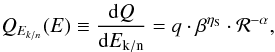
Results. Proton data are well described in the simplest model defined by a power-law source spectrum and plain diffusion. They can also be accommodated by models with, e.g., convection and/or reacceleration. There is no need for breaks in the source spectral indices below ~1 TeV/n. Fits to the primary fluxes alone do not provide physical constraints on the transport parameters. If we leave the source spectrum free, parametrised by the form dQ/dE = qβηSℛ−α, and fix the diffusion coefficient K(R) = K0βηTℛδ so as to reproduce the B/C ratio, the MCMC analysis constrains the source spectral index α to be in the range 2.2−2.5 for all primary species up to Fe, regardless of the value of the diffusion slope δ. The values of the parameter ηS describing the low-energy shape of the source spectrum are degenerate with the parameter ηT describing the low-energy shape of the diffusion coefficient: we find ηS − ηT ≈ 0 for p and He data, but ηS − ηT ≈ 1 for C to Fe primary species. This is consistent with the toy-model calculation in which the shape of the p/He and C/O to Fe/O data is reproduced if ηS − ηT ≈ 0−1 (no need for different slopes α). When plotted as a function of the kinetic energy per nucleon, the low-energy p/He ratio is determined mostly by the modulation effect, whereas primary/O ratios are mostly determined by their destruction rate.
Conclusions. Models based on fitting B/C are compatible with primary fluxes. The different spectral indices for the propagated primary fluxes up to a few TeV/n can be naturally ascribed to transport effects only, implying universality of elemental source spectra.
Key words: methods: statistical / cosmic rays
Appendix A is only available in electronic form at http://www.aanda.org
© ESO, 2011
1. Introduction
The measured Galactic cosmic-ray (GCR) fluxes at Earth result from a three-step journey: i) the diffusive shock acceleration (DSA) mechanism provides a source spectrum; ii) these particles are then transported (by diffusion, but also convection and reacceleration) and also interact in the interstellar medium (ISM) until they reach the Solar neighbourhood; iii) they enter the solar cavity where they decelerate due the effect of solar modulation (active for GCRs below a few tens of GeV/n).
The last step prevents direct measurements of low-energy (beyond a few hundreds of GeV/n) interstellar fluxes (IS). The first step can be investigated by means of semi-analytical or numerical studies of the DSA mechanism. However, due to the variety of possible sources for the GCRs, and the intrinsic complexity of this mechanism, the source spectral index and especially its low-energy shape is not very well predicted (e.g., Caprioli et al. 2010). Awaiting further progress along this line, an indirect route to access the source spectrum is to start with the top-of-atmosphere (TOA) fluxes and go back to the source spectra. To do so, it is generally assumed that the steady state holds for the propagation, and that the first and second step are independent. The first assumption is known to fail at high enough energies, whereas the second one may only be approximate. In this study, given the success of simple steady-state diffusion models for the nuclear component, we follow the same route in order to draw some constraints on the source parameters. Note that this paper does not consider primary electrons, whose spectrum may depend on local sources above a few tens of GeV (e.g., Boulares 1989; Delahaye et al. 2010).
The propagation step is the focal point of many phenomenological studies addressing the flux of secondary species (created by interactions of the primary species in the ISM and radiation fields of the Galaxy) including light nuclei, antiprotons, positrons, radioactive isotopes and also gamma rays. The transport parameters are usually determined by fitting data on secondary-to-primary ratios of nuclei, as for example the B/C (boron-to-carbon) ratio. However, present data on B/C ratio, even when combined with CR radioactive isotope measurements, lead to a constrained but large range of allowed values for these parameters (Maurin et al. 2001, 2010; Putze et al. 2010). The study of these secondary-to-primary ratios is – to first order – insensitive to the details of the source spectra (e.g., Maurin et al. 2002). Therefore, a common phenomenological approach is to first extract the transport parameters, then to fit the source spectra; however the source and transport parameters may be correlated (Putze et al. 2009).
The importance of the primary fluxes and their ratios was recognised a long time ago (Webber & Lezniak 1974). In this paper we reconsider their study, trying to answer the following questions: what phenomena shape the TOA and IS fluxes? Is it the source spectrum or the propagation step, and are there degeneracies between the two effects? To what accuracy can we determine the low-energy source spectra, the spectral indices, and the source abundances? Are the source spectra universal or species-dependent?
On the experimental side, accurate data are available up to a few hundreds of GeV, whilst at higher energies data are less abundant and have large error bars and scatter between experiments. On the modelling side, we have a semi-analytical propagation model proved to work well with many GCR observables (Maurin et al. 2001; Donato et al. 2001, 2002, 2009) and an implementation of the Markov Chain Monte Carlo technique (MCMC) to derive the probability density functions of the analysed model parameters (Putze et al. 2009, 2010). We take advantage of these to address the above questions. Our results are also supported by toy-model calculations, especially for the shape of ratio p/He. As abundant and accurate data are expected in the near future by the orbiting PAMELA experiment and forthcoming AMS-02 detector (to be installed on the International Space Station), such a study also aims at providing some guidelines on how to tackle the information contained in the primary flux propagated spectra. We finally note that the recent ATIC-2 and CREAM-I measurements for proton and Helium data hint at a spectral change ≳ TeV/n. This has consequences for the secondary production of γ-rays, antiprotons, and positrons (Donato & Serpico 2010; Lavalle 2010). However, this occurs only for the high-energy part of these spectra. In particular, as our previous antiproton calculations (Donato et al. 2001) relied on a fit to the data, the conclusions obtained in Donato et al. (2008) remain unchanged even with the new source spectra provided in this study.
The paper is organised as follows: Sect. 2 contains a short overview of the propagation scheme employed in the present study. In Sect. 3, we discuss the p and He data and whether they can provide any constraints on the transport parameters or if they can be fitted in any propagation configuration (e.g. with or without convection, with or without reacceleration). In Sect. 4, we seek for generic constraints on the source spectra (p, He, and C to Fe) comparing the values obtained in different configurations of propagation models. In Sect. 5, the origin for the observed shape for the ratio of primary species is outlined. Our conclusions and perspectives are given in Sect. 6.
2. The propagation model
The framework employed to calculate the fluxes is the diffusion model with convection and reacceleration discussed in Maurin et al. (2001, 2002), updated and fully detailed in Putze et al. (2010). Here we only summarise the main features of the model.
The Galaxy is shaped as a gaseous thin disk with half-thickness h = 0.1 kpc and an infinite radial extension (1D model, as also used in Jones et al. 2001), hosting the interstellar medium and the stars, and surrounded by a thick halo for cosmic-ray transport whose half-height is L.
Assuming a steady-state situation, the transport equation for the CR
nucleus j can be written as
 (1)where the differential density
Nj ≡ Nj(E,r)
depends on the position r in the Galaxy and on the energy
(throughout the paper, E is the total energy,
Ek is the kinetic energy, Ek/n the
kinetic energy per nucleon, and E/n the total energy per
nucleon). ℒj sums up the physics of the transport in the Galaxy,
while
(1)where the differential density
Nj ≡ Nj(E,r)
depends on the position r in the Galaxy and on the energy
(throughout the paper, E is the total energy,
Ek is the kinetic energy, Ek/n the
kinetic energy per nucleon, and E/n the total energy per
nucleon). ℒj sums up the physics of the transport in the Galaxy,
while  contains the source term.
2.1. Transport parameters
The operator ℒ (we omit the superscript j) describes the
diffusion K(r,E) and
convection VC(r) in
the Galaxy, the decay rate
Γrad(E) = 1/(γτ0)
for radioactive species, and the destruction rate
Γinel(r,E) = ∑ ISMnISM(r)vσinel(E)
on the interstellar matter (ISM). It reads
 (2)The spatial diffusion coefficient is
parametrised as
(2)The spatial diffusion coefficient is
parametrised as 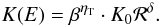 (3)where ℛ = pc/Ze is the rigidity of the
particle, β is the velocity of the particle in units of c
and ηT parameterizes the low-energy behaviour of diffusion.
The nominal form is given by ηT = 1, which is just the
inevitable effect of particle velocity on the diffusion rate. Hence this
β term is always present, and other values
of ηT are relative to this. Ptuskin et al. (2006) argued that the form of the spatial diffusion coefficient
could be modified at low energy, due to the possibility that the nonlinear MHD cascade
sets the power-law spectrum of turbulence. Indeed, Maurin
et al. (2010) found that the value of this parameter was crucial for the
determination of δ given the current B/C data. The convective wind acts
in the whole diffusive volume with a constant velocity
VC = ± VCeZ
pointing perpendicularly to the Galactic disk. The coefficients b
and c account for the first and second order energy changes
(3)where ℛ = pc/Ze is the rigidity of the
particle, β is the velocity of the particle in units of c
and ηT parameterizes the low-energy behaviour of diffusion.
The nominal form is given by ηT = 1, which is just the
inevitable effect of particle velocity on the diffusion rate. Hence this
β term is always present, and other values
of ηT are relative to this. Ptuskin et al. (2006) argued that the form of the spatial diffusion coefficient
could be modified at low energy, due to the possibility that the nonlinear MHD cascade
sets the power-law spectrum of turbulence. Indeed, Maurin
et al. (2010) found that the value of this parameter was crucial for the
determination of δ given the current B/C data. The convective wind acts
in the whole diffusive volume with a constant velocity
VC = ± VCeZ
pointing perpendicularly to the Galactic disk. The coefficients b
and c account for the first and second order energy changes
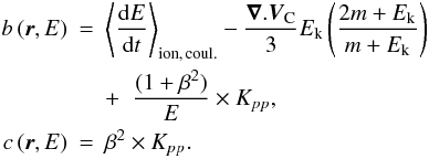 Coulomb and ionisation losses add to possible
energy gains due to reacceleration, described by the
coefficient Kpp in momentum space. The
parameterisation for Kpp is taken from the
model of minimal reacceleration by the interstellar turbulence (Osborne & Ptuskin 1988; Seo &
Ptuskin 1994):
Coulomb and ionisation losses add to possible
energy gains due to reacceleration, described by the
coefficient Kpp in momentum space. The
parameterisation for Kpp is taken from the
model of minimal reacceleration by the interstellar turbulence (Osborne & Ptuskin 1988; Seo &
Ptuskin 1994): 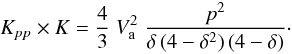 (4)where Va is the
Alfvénic speed.
(4)where Va is the
Alfvénic speed.
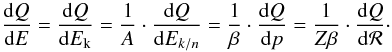
2.2. Source parameters
The source term  includes the initial spectrum at the sources and the secondary contributions (spallations
of heavier nuclei). Acceleration models typically predict
dQ/dp ∝ p−α
(e.g., Jones 1994), which leads to
dQ/dE ∝ p−α/β,
where the low-energy behaviour is unknown. For future reference, we note that
includes the initial spectrum at the sources and the secondary contributions (spallations
of heavier nuclei). Acceleration models typically predict
dQ/dp ∝ p−α
(e.g., Jones 1994), which leads to
dQ/dE ∝ p−α/β,
where the low-energy behaviour is unknown. For future reference, we note that
 (5)In this paper, we model the low-energy shape
by adding one free parameter, ηS, active at low energy:
(5)In this paper, we model the low-energy shape
by adding one free parameter, ηS, active at low energy:
 (6)where q is taken to be the
normalisation for a differential energy per nucleon source spectrum. The reference
low-energy shape corresponds to ηS = −1 (to have
dQ/dp ∝ p−α,
i.e. a pure power-law).
(6)where q is taken to be the
normalisation for a differential energy per nucleon source spectrum. The reference
low-energy shape corresponds to ηS = −1 (to have
dQ/dp ∝ p−α,
i.e. a pure power-law).
2.3. Free parameters of the model
The present model contains of necessity several free parameters: the parameters in the transport sector {K0, δ, Va, Vc, ηT} , the ones in the source term {q, ηS, α} , and the halo size of the Galaxy L in the geometry sector. We will see in the following that not all these parameters have the same relevance to the physics of primary cosmic nuclei, and we will therefore operate within a critical sub-range of parameters. In diffusion models, L cannot be solely determined from the B/C ratio because of the well-known degeneracy between K0 and L when only stable species are considered. If not differently stated, we will work with the default values ηS = −1 and ηT = 1, and the reference value L = 4 kpc. In most of the analyses we let free the source normalisation qi for each primary species.
The low energy (≲10 GeV/n) charged particles are braked in the heliosphere by the solar
wind, modulated with variations of the scale of the 11-year cycle. We adopt the
force-field approximation, which provides a simple analytical one-to-one correspondence
between the modulated top-of-the atmosphere (TOA) and the demodulated interstellar (IS)
fluxes, and whose only effective parameter is the modulation
potential φ (GV). For a species j, the IS and
TOA energies per nucleon are related by  (Φ = Z/A × φ is the modulation
parameter), and the fluxes by (p is the momentum)
(Φ = Z/A × φ is the modulation
parameter), and the fluxes by (p is the momentum)  (7)The force-field method is an approximated
solution to the diffusion equation for charged particles in the heliosphere. A more
accurate treatment is far beyond the scope of our paper, which is centred on the source
and diffusive processes active in much a wider energy range and responsible for strong
effects of the primary spectra.
(7)The force-field method is an approximated
solution to the diffusion equation for charged particles in the heliosphere. A more
accurate treatment is far beyond the scope of our paper, which is centred on the source
and diffusive processes active in much a wider energy range and responsible for strong
effects of the primary spectra.
In principle, the solar modulation potential could also be a free parameter of the study. Since the low-energy spectrum of the primary fluxes is determined mainly by the low-energy injection spectrum (see Eq. (6)), the low-energy diffusion scheme (see Eq. (3)), and the solar modulation (see Eq. (7)), a non-trivial correlation is expected between these parameters. For instance, we find using the minuit minimisation routines (not shown) that there is a negative correlation between φ and ηS. This holds for all primary cosmic-ray fluxes studied in this work. Given that there is already a great number of degeneracies between the different source parameters, which cannot be lifted with the current available data, we choose to fix the modulation potential φ to the values given by the experiments. A more detailed study, in the spirit of the one done in Trotta et al. (2010), will be undertaken in a future work.
3. Analysis with free source and transport parameters
In this section, we use different data sets for proton and helium fluxes1 in order to determine which propagation models describe data and to try to set constraints on the free parameters of our model. The fitting procedure is based on the minuit routine, which minimises a χ2 function.
3.1. Data
A first important consideration is the choice of the data used to constrain the models.
The top panel in Fig. 1 shows the available data
for p and He fluxes. The abscissa is the kinetic energy per
nucleon (Ek/n) and the ordinate
ψIS ×  , where ψIS is
the IS, demodulated using the force-field approximation. The low-energy region (below
100 GeV/n) has been covered by many balloon-borne, Space-Shuttle based and satellite
experiments, whereas above a few TeV/n the data come from several balloon long-exposure
flights (accumulated over several flights in a decade). ATIC data cover the gap at a few
TeV/n energy. The overall agreement between the data is fair, the scatter between the data
being higher at high energy.
, where ψIS is
the IS, demodulated using the force-field approximation. The low-energy region (below
100 GeV/n) has been covered by many balloon-borne, Space-Shuttle based and satellite
experiments, whereas above a few TeV/n the data come from several balloon long-exposure
flights (accumulated over several flights in a decade). ATIC data cover the gap at a few
TeV/n energy. The overall agreement between the data is fair, the scatter between the data
being higher at high energy.
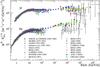 |
Fig. 1 Demodulated p and He data ( |

For our analysis, the criterion is to select data samples covering a broad energy range and consistent between experiments. We show a subset of demodulated data in Fig. 2 to illustrate the error bars and differences between the most recent and consistent sets of p and He data, namely AMS-01 (Alcaraz et al. 2000; AMS Collaboration et al. 2000), BESS98 (Sanuki et al. 2000; Shikaze et al. 2007) and BESS-TeV (a.k.a. BESS02, Haino et al. 2004; Shikaze et al. 2007). For the proton flux, the AMS-01 and BESS98 data, both taken in 1998 in the same solar period, are consistent except at low energy. BESS-TeV data taken in 2002 during a high level of solar activity show a different behaviour at low and intermediate energies. Note that usually the solar modulation level is obtained by fitting φ and a simple two-parameter proton spectrum to the data (Shikaze et al. 2007). This is the standard lore in the field, although it is expected to give a biased modulation level (for example, we do not know the true interstellar proton spectrum, there is the problem of polarity in the solar magnetic field, etc.). The use of demodulation has the same physical basis as modulating in the same scheme (the force-field in our case, see Eq. (7)). In Figs. 1 and 2 we have chosen to demodulate data to compare all existing data on the same foot. Since the solar modulation is effective up to few GeV/n, only the very low side of the figures are affected by the demodulation procedure. The goal of this paper is not to deal with these issues, but simply the fact that the proton data are already inconsistent among themselves implies that we may expect inconsistencies in the fitted models.
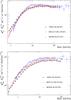 |
Fig. 2 Demodulated p (top panel) and He (bottom panel)
flux |
3.2. Pure diffusive transport
The first step is to test a minimal model containing only acceleration and plain diffusion, as well as nuclear reactions and electromagnetic energy losses, but without convection and reacceleration (Va = Vc = 0).
Main degeneracies.
In the pure diffusion model, the flux of any primary species at high energy can be
approximated by2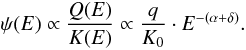 (8)This formula shows two degeneracies between
the source and transport parameters: the first one is in the
normalisation q/K0, the second one is in
the total spectral index α + δ.
(8)This formula shows two degeneracies between
the source and transport parameters: the first one is in the
normalisation q/K0, the second one is in
the total spectral index α + δ.
We start with a minimisation procedure setting the free parameters δ,α
and qp,He (in order to break the degeneracy
between q and K0 the latter is set to
0.0048 kpc2 Myr-1). The results for protons and helium are
presented in two different columns in Table 1.
The  values are very small for a number of
cases, indicating a possible over-fitting of the data. The values of the best-fit
parameters are not reported since they are not relevant at this stage of the analysis.
For the different sets of data, the values of both α
and δ vary from almost any value between 0 and 2.8 (not shown in the
table), but the sum of them is close to 3.0 for p and 2.8 for He. The first three lines
show that a fit to p and He on the AMS or BESS data is always possible in a simple
diffusion scheme (although it provides unphysical values for α
and δ). The fourth line shows the combined analysis of AMS-01 (Alcaraz et al. 2000) and BESS98 (Sanuki et al. 2000) data. They were collected in the same year (1998)
– which may help reduce the systematics due to solar wind modelling – and span nearly
the same energy range. The
values are very small for a number of
cases, indicating a possible over-fitting of the data. The values of the best-fit
parameters are not reported since they are not relevant at this stage of the analysis.
For the different sets of data, the values of both α
and δ vary from almost any value between 0 and 2.8 (not shown in the
table), but the sum of them is close to 3.0 for p and 2.8 for He. The first three lines
show that a fit to p and He on the AMS or BESS data is always possible in a simple
diffusion scheme (although it provides unphysical values for α
and δ). The fourth line shows the combined analysis of AMS-01 (Alcaraz et al. 2000) and BESS98 (Sanuki et al. 2000) data. They were collected in the same year (1998)
– which may help reduce the systematics due to solar wind modelling – and span nearly
the same energy range. The  for the fit of combined He data,
compared to the corresponding values of 0.72 and 0.36 for the separate
data shows inconsistencies among the data sets, as underlined in Sect. 3.1. When combining the three experiments (fifth line),
this is even more visible, also for protons (the best-fit slope is unaffected). We have
fitted also all the available data in the low energy (sixth line) and in the highest
energy range (last line). The agreement among the data sets is poor, both for protons
and helium, as already visible in Fig. 1.
ATIC data, which connect the low and high energy sectors, are badly fit by any pure
diffusive model.
for the fit of combined He data,
compared to the corresponding values of 0.72 and 0.36 for the separate
data shows inconsistencies among the data sets, as underlined in Sect. 3.1. When combining the three experiments (fifth line),
this is even more visible, also for protons (the best-fit slope is unaffected). We have
fitted also all the available data in the low energy (sixth line) and in the highest
energy range (last line). The agreement among the data sets is poor, both for protons
and helium, as already visible in Fig. 1.
ATIC data, which connect the low and high energy sectors, are badly fit by any pure
diffusive model.
Best-fit to p and He data for pure diffusive transport.
We may naively interpret the results of Table 1 as showing that p and He data can be well accommodated in any purely diffusive transport models, in the low energy range (≲100 GeV/n), for each experimental data set taken separately. But such models lead to unphysical values for δ and α. So it could also mean that the hypothesis of a standard source spectrum (i.e., dQ/dp ∝ ℛ−α when setting ηS = −1) and a standard propagation scheme (ηT = 1) is unsupported by the data, or that additional effects (e.g., convection and/or reacceleration) are required to match the data. Before resolving this issue, we go further with the comparison of the approximate formulae and the full calculation.
Inelastic interaction: a link between α, δ and K0.
Explicitly, the effect of the catastrophic losses at low energy, Eq. (8) gives, for a 1D model, 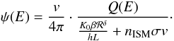 (9)For δ fixed, Eq. (9) implies a correlation
between K0, α and δ,
given some primary data. Indeed, as K0 decreases,
the inelastic interaction term nISMσv
becomes more efficient in the denominator of Eq. (9). The effect of species destruction is therefore more pronounced
at low energy. Fixing δ and going to
small K0 we expect that, in order to balance the increased
destruction rate, the numerator compensates but increasing α.
If K0 is fixed and small, so that inelastic interactions
can dominate, the same flux of protons (or helium) can be obtained with a
larger α + δ.
(9)For δ fixed, Eq. (9) implies a correlation
between K0, α and δ,
given some primary data. Indeed, as K0 decreases,
the inelastic interaction term nISMσv
becomes more efficient in the denominator of Eq. (9). The effect of species destruction is therefore more pronounced
at low energy. Fixing δ and going to
small K0 we expect that, in order to balance the increased
destruction rate, the numerator compensates but increasing α.
If K0 is fixed and small, so that inelastic interactions
can dominate, the same flux of protons (or helium) can be obtained with a
larger α + δ.
This effect is confirmed by the numerical results, as seen in Fig. 3. For each point in the K0 − δ plane, we plot α + δ for the best-fit model on AMS-01 proton data (the free parameters are α and qp). We checked (not shown) that similar values for α + δ are obtained when the fits is performed on other proton fluxes (BESS98 or BESS-TeV), or for other species (He or a combined fit p+He). We can see from the figure that, for any fixed δ value, the data require higher α + δ while K0 decreases, due to the increasing importance of the destruction rate. This effect is less pronounced for small values of the diffusion coefficient slope, namely when δ is close to 0.2−0.3.
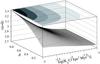 |
Fig. 3 Surfaces of α + γ for the best-fit models in the plane K0 − δ (free parameters are α and qp) on AMS-01 proton data. The colour code (from light to darker shades) for the contours superimposed on top of each graph correspond to (α + γ) = {2.8, 2.9, 3.0, 3.1, 3.2}. |
Asymptotic behaviour (or why α + δ ≳ γdata).
Even for light primary species such as protons, which suffer less from destruction in
the ISM, the asymptotic purely diffusive regime is not reached. If we fit a primary flux
with (as is usually done in the literature) 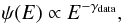 then we are bound to have
 This implies that caution is in order
whenever we wish to compare the result of studies fitting the propagated fluxes with a
power-law function (e.g., Shikaze et al. 2007) to
those (such as this one) fitting directly the source spectrum. Catastrophic, but also
continuous losses flatten the propagated spectrum below ≲few tens of GeV/n energies.
The inequality γasympt ≳ γdata
is also valid for convection and/or reacceleration, as derived from an analysis of B/C
(Putze et al. 2010; Maurin et al. 2010).
This implies that caution is in order
whenever we wish to compare the result of studies fitting the propagated fluxes with a
power-law function (e.g., Shikaze et al. 2007) to
those (such as this one) fitting directly the source spectrum. Catastrophic, but also
continuous losses flatten the propagated spectrum below ≲few tens of GeV/n energies.
The inequality γasympt ≳ γdata
is also valid for convection and/or reacceleration, as derived from an analysis of B/C
(Putze et al. 2010; Maurin et al. 2010).
Simultaneous fit of p and He to lift the α + δ degeneracy?
As the residence time – hence the destruction rate of any species – depends on the
energy through the transport parameter δ (and not on
α + δ), the different inelastic cross-sections for
each species ( mb and
 mb) leave different imprints on the
corresponding p and He low-energy spectra. This is expected, to some degree, to lift the
degeneracy on α + δ when using a combined fit to
various primary species.
mb) leave different imprints on the
corresponding p and He low-energy spectra. This is expected, to some degree, to lift the
degeneracy on α + δ when using a combined fit to
various primary species.
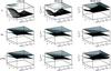 |
Fig. 4 Surfaces of |
Figure 4 shows the
contours in the
K0 − δ plane for the separate fits of p
(first row), He (second row) and for the combined fit p+He (last row), for the different
sets of data used before. The ranges chosen for K0
and δ correspond to extreme but not impossible values of these
parameters that can accommodate the secondary-to-primary B/C ratio (Maurin et al. 2010). The top-left plot shows the
strong degeneracy of α and δ (for AMS-01 data),
as almost any configuration is acceptable. The top-right plot shows that for other data
(BESS-TeV) no good fit can be achieved ( ) in the selected
K0 − δ region: the good fits occur for
unrealistic δ only. We note here that there is no inconsistency with
the results shown in Table 1, which have been
obtained by spanning larger ranges for the free parameters including unphysical values.
The second row of Fig. 4 shows the fits to He data.
All the experiments tend to prefer large K0 and
large δ (both unrealistic if we demand
~ 1), but
the χ2 does not change significantly, meaning that no
particular class of models is selected by the helium data.
) in the selected
K0 − δ region: the good fits occur for
unrealistic δ only. We note here that there is no inconsistency with
the results shown in Table 1, which have been
obtained by spanning larger ranges for the free parameters including unphysical values.
The second row of Fig. 4 shows the fits to He data.
All the experiments tend to prefer large K0 and
large δ (both unrealistic if we demand
~ 1), but
the χ2 does not change significantly, meaning that no
particular class of models is selected by the helium data.
The third row of Fig. 4 is the combined p+He fit.
The resulting surfaces corresponds to a trade-off
between the best-fit for p and He. The best-fit δ (not shown in the
figure) still falls in region of δ ≳ 1, and the
degeneracy α + δ is not lifted as no specific value
for δ is preferred.
The role of ηS and ηT.
We have introduced the possibility to have a non-standard low-energy diffusion
coefficient by means of the parameter ηT, as given by
Eq. (3). The low-energy shape of the
source spectrum is driven by the parameter ηS, see
Eq. (6). If for illustration we neglect
the nuclear interactions, we obtain 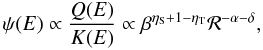 (10)where the extra β factor
comes from the v/4π in front of Eq. (9).
(10)where the extra β factor
comes from the v/4π in front of Eq. (9).
The parameters ηS and ηT introduce a similar shape correction at the lowest energies. If it were not for energy losses and inelastic reactions (see next section), only the quantity ηS − ηT would be expected to be constrained. We fit AMS-01 and BESS98 data, as well as all the proton data, with α, ηS, δ, and qp as free parameters. The best χ2 is slightly smaller than the one obtained with only α, δ, and qp free (and ηS = −1). Similar results are achieved when the acceleration scheme is fixed to the standard lore (ηS = −1) and the fourth free parameter is ηT. However, the corresponding values for δ and α are again unsupported.
A further degeneracy can be produced by solar modulation, whose action is a decrease of the flux with the increase of the solar wind strength (parameter φ). On the other hand, the TOA flux increases with φ when ηS ≤ ηT (in the standard scenario ηs = −1 and ηT = 1), so that some compensation of the solar modulation can be produced.
3.3. Summary for the transport parameter constraints from p and He data
The existing proton and helium data are unable to select any particular propagation model. This is consistent with the fact that the transport and source parameters are degenerate, as shown from simple arguments in our toy formulae. The best present data (AMS-01, BESS98 and BESS-TeV) can be quite well reproduced by solar modulated pure diffusive transport for instance, but they favour unphysical values of the source and transport parameters. Hence other ingredients are required. This could be a modification of the low-energy source spectrum or diffusion coefficient, or the addition of convection and/or reacceleration (which can also accommodate the current data), or an improvement of the calculation of the solar modulation effect. However, given the present data and the physics of primary spectra, such an approach is bound to fail: the increase of the parameter space merely brings new degeneracies. Moreover, most of the parameter space is already ruled out by the constraints from the B/C ratio. To go further, we thus have to restrict the parameter space to the source parameter space only (and use some prior on the propagation parameters).
4. Analysis with fixed transport parameters
In the previous sections we have shown that present data on primary fluxes alone cannot constrain significantly the transport parameters. The next natural strategy is to fit simultaneously primary and secondary species. However, as emphasised in Putze et al. (2009), the large body of data for primary species drives the fit away from the best-fit regions of the B/C ratio. Actually, the standard lore is to fix the transport parameters to their best-fit value, and then constrain the source parameters. But the latter values are then biased3. We nevertheless follow this approach, but we repeat the analysis on several possible transport configurations. This allows us to derive explicitly the systematic effects of the source parameters arising from this bias.
In this section, we first gather several sets of transport parameters shown to be consistent with B/C data (Sect. 4.1). We then fit the source parameters for p and He, the best-measured primary fluxes to date (Sect. 4.2). We repeat the analysis for other primary species, to inspect the universality of the source slopes and obtain their relative source abundances (Sect. 4.3).
4.1. Transport parameters consistent with B/C
The transport parameters are usually constrained from secondary-to-primary ratios (e.g. B/C). In the literature, various classes of models have been used, leading to very different values of their respective best-fit parameters (see, e.g., Strong et al. 2007, for a review). For instance, a model with diffusion + reacceleration is characterised by a best-fit propagation slope δ ≈ 0.3−0.4 (e.g., Lionetto et al. 2005), leaky-box inspired models points to δ ≈ 0.5−0.6 (e.g., Webber et al. 2003; Putze et al. 2009), whereas diffusion + convection models (w/wo reacceleration) points to δ ≈ 0.75−0.85 (e.g., Maurin et al. 2001; Putze et al. 2010).
This sensitivity to the CR transport mode (pure diffusion, w/wo convection, w/wo reacceleration) is discussed in Maurin et al. (2010). Although the best-fit model is one with both convection and reacceleration, it predicts δ ~ 0.8, a value quite high compared with theoretical expectations (1/3 for a Kolmogorov spectrum of turbulence, and 1/2 for Kraichnain, e.g., Strong et al. 2007). Following Maurin et al. (2010), we use below four configurations of the diffusion model covering a large but plausible range for the transport parameters. These models along with their best-fit parameters are reproduced in Table 2:
-
model II is with reacceleration only;
-
model III is with convection and reacceleration;
-
model I/0 is with a low-energy upturn of the diffusion coefficient (ηT < 0);
-
model III/II is as I/0, but with reacceleration.
The first two models correspond to the best-fit parameters for a standard spatial
diffusion coefficient (i.e. ηT set to 1, see Eq. (3)). The last two lines correspond to a
modified diffusion scheme: negative values of ηT are
associated to an upturn of the diffusion coefficient at low energy (Ptuskin et al. 2006). These two models are respectively termed I/0
and III/II because both allow some convection, but both favour
 . As shown in Fig. 6 of Maurin et al. (2010), these
models fit reasonably well the B/C data.
. As shown in Fig. 6 of Maurin et al. (2010), these
models fit reasonably well the B/C data.
Best-fit transport parameters for various configurations of the diffusion model (fitted on B/C data).
4.2. Constraints on p and He source parameters
4.2.1. Generalities
On the one hand, the low-energy shape of the source spectra are not well known theoretically. They result from the diffusive shock acceleration mechanisms at play in supernova (e.g. Drury 1983) or super-bubble shocks (e.g. Ferrand et al. 2008; Ferrand & Marcowith 2010). Power-laws close to −2 (in energy space) are predicted at high energy, but there is still no agreement about the low-energy spectrum (e.g. Caprioli et al. 2010).
On the other hand, we have access only to propagated spectra, where effects such as destruction on the ISM, energy losses, Galactic winds and reacceleration change the energy spectra up to a few tens of GeV/n. This is the route followed in this section, where we try to constrain the source parameters from a fit to the propagated fluxes. However, the shape of the flux at low-energy is only an extrapolation since the low-energy interstellar spectrum is masked by solar modulation effects.
Note that the low-energy (below 100 MeV) IS spectrum can be indirectly constrained due to its interaction with the interstellar medium. In this approach, the IS flux is based on empirical fits to the data (e.g., Herbst et al. 2010), and its extrapolation at low energy is used to calculate, e.g., the ionisation of the ISM (Webber 1987; Nath & Biermann 1994; Webber 1998) or of molecular clouds (Padovani et al. 2009), or the LiBeB Galactic enrichment and production (Gilmore et al. 1992; Nath & Biermann 1994; Lemoine et al. 1998). Some of these studies find an increase in the low-energy spectrum, others a decrease (with respect to a pure power law). Actually, data from the Voyager 1 & 2 spacecraft near the heliospheric termination shock could also be helpful for such studies, as they are close to interstellar conditions, their level of modulation being ≈60 MV (Webber et al. 2008; Webber & Higbie 2009). However, it has been argued recently that anomalous cosmic rays could contribute to an important fraction of the proton spectrum below 300 MeV (Scherer et al. 2008). For this reason, we do not include Voyager data in our fits, and will only compare them to the best-fit spectra (based on the other data) at the end of this section.
4.2.2. Results
Due to the lack of robust information about the low-energy spectrum, we choose to rely
on a simple parametrisation allowing for an increase or decrease at low-energy, as given
by Eq. (6),
i.e. QEk/n(E) = q·βηS·ℛ−α.
For each configuration given in Table 2 – i.e.,
for a given choice of the transport parameters K0,
δ, ηT, Va,
and Vc – we then use the MCMC technique to get the
probability density function (PDF)4 of the three
source parameters qi,
 and αi (where i is
either p or He). The three data sets on which we base the analysis are AMS-01, BESS98
and BESS-TeV (see Sect. 3).
and αi (where i is
either p or He). The three data sets on which we base the analysis are AMS-01, BESS98
and BESS-TeV (see Sect. 3).
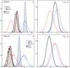 |
Fig. 5 Left panels: PDF of the source slope α for p (unfilled histograms) and He (hatched histograms). Right panels: PDF for αHe − αp. The colour code corresponds to the three experimental data used: AMS-01 (solid black line), BESS98 (dashed red lines) and BESS-TeV (dash-dotted lines). |
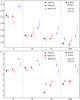 |
Fig. 6 Most-likely value (symbols), 68% and 95% CIs for p (filled symbols) and He (open symbols) for the four propagation configurations gathered in Table 2. Top panel: spectral index α. Bottom panel: low-energy source parameter ηS (see Eq. (6)). The grey line ηS = −1 corresponds to the value for which the source spectrum is a pure power-law in rigidity (i.e. dQ/dℛ ∝ ℛ−α). |
PDF of αp, αHe, and αHe − αp.
The two left panels of Fig. 5 show the PDF of αp (hatched histograms) and αHe (empty histograms), whereas the two right panels show the PDF of αHe − αp to visually inspect any discrepant spectral index for the two species. For AMS-data (solid black lines), both model II (reacceleration, δ = 0.23) and model III (reacceleration and convection, δ = 0.86) show a very good agreement between their p and He spectral index, with respectively αII ≈ 2.45 and αIII ≈ 2.3. There are significant differences for BESS98 (red dashed lines) and BESS-TeV (blue dash-dotted lines) data: first, the match between αHe and αp is not as good as for AMS-01, yet αHe − αp remains marginally consistent with 0. The plots on the right panels and the width of the PDF tell us that the data current precision does not allow us to separate differences ≲0.1 in the spectral indices.
The 68% and 95% CIs on the spectral indices for the four transport configurations of Table 2 and the three sets of data are shown in the top panel of Fig. 6. From a quick visual inspection, the following trends are found:
-
for any given data set and species(p or He),the spread in the source slopes isαp − αHe ≲ 0.2, regardless of the model (values in the same column in Table 3);
-
for any given model, the typical spread in α when fitting different data sets (values in the same row in Table 3) is ≈0.05 for αp and ≈0.1 for αHe. This is larger than the errors extracted from the minuit minimisation routine, which gives a statistical uncertainty αp − αHe ≲ 0.01 (not shown);
-
the spectral indices obtained from BESS-TeV data are systematically larger and marginally incompatible with those found for AMS-01 and BESS98. This may be related to the systematically higher value obtained for ηS (see below);
-
model II (reacceleration only) gives larger spectral indices, inconsistent with the values found for the three other models. This is not unexpected as it has the smallest δ of all models (considered in Table 2).
A scatter of ~0.2 is thus attributed to the fact that we do not know which model is best, and a scatter ~0.1 because of systematics in the data.
Low energy and confidence intervals (CIs) on ηS.
The 68% and 95% CIs on the parameter ηS controlling the low-energy behaviour of the source spectrum5 are shown for the same models/data in the bottom panel of Fig. 6. BESS-TeV data being at slightly higher energy than AMS-01 and BESS98, its source spectrum low-energy parameter ηS is less constrained. Otherwise, the p and He ηS point to fairly similar values for any given propagation configuration. However, this value depends on the model chosen: the reacceleration model (II) and convection/reacceleration model (III) both favour ηS ≈ 1, whereas ηS is close to −2 for model I/0 and −1.5 for model III/II. The latter value is consistent with a source spectrum being a pure power-law in rigidity, whereas the former value implies a flattening at low energy. This is understood if we inspect the quantity ηS − ηT, appearing in Eq. (10): for models II and III that have ηT = 1, this give ηS − ηT ≈ 0. For models I/0 and III/II that have respectively ηT = −2.6 and −1.3, this gives ηS − ηT ≈ 0.6 and −0.2. So it seems that the constraint ηS − ηT ≈ 0 should be met for any propagation model.
Source abundances qi.
The scatter is quite large when all the different models/data are considered. The absolute values are not meaningful since they depends on the choice of L that is arbitrary set to 4 kpc in this analysis. We nevertheless note that the ratio qHe/qp falls in the range 0.3−0.6 (not shown), with a typical spread of ≈0.1−0.2 for the PDF.
 |
Fig. 7 TOA (modulated) fluxes (times |
Best-fit spectral index α for p and He fit and associated
.
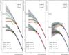 |
Fig. 8 95% CL envelopes for the proton and helium fluxes for the four propagation configurations of models of Table 2. The three panels correspond respectively to the result of the MCMC analysis on AMS-01 data (left panel), BESS98 data (middle panel), and BESS-TeV (right panel). For the sake of comparison, the IS (demodulated) AMS-01 (black circles), BESS98 (red squares), BESS-TeV (blue triangles), along with the Voyager data (stars). |
Spectra, goodness of fit, and high-energy asymptotic regime.
The data along with the best-fit spectra for all models are shown in Fig. 7. An eye inspection shows a good match to the data.
More precisely, the values given in Table 3 tell us that the fit to the data is very good for
BESS98 and BESS-TeV, but not satisfactory for most of the models with AMS-01 data
(for which the first and last two bins are not well reproduced given their small error
bars). We remark that the spread in δ is larger than the spread
in α (see above). Hence, the smaller δ,
the smaller
γasympt(= α + δ). This
is consistent with the same ordering for all species of the propagated spectra – from
larger to smaller γasympt – seen in Fig. 7. The top curve is always model II
(δ = 0.23, solid lines), going down to model III/II
(δ = 0.51, long dash-dotted lines), model I/0
(δ = 0.61, dashed lines), and then model III
(δ = 0.86, short dash-dotted lines) for the bottom curve. This
emphasises that more accurate data in the high energy regime (TeV-PeV) are needed to
better constrain the asymptotic behaviour.
Envelopes on IS fluxes and consistency with low-energy Voyager data.
Finally, the three panels of Fig. 8 show the envelopes on the IS fluxes (obtained from the 95% CIs on the parameters). The flux is extrapolated down to an IS energy of ~0.1 GeV/n, where the demodulated Voyager energies fall (Webber & Higbie 2009)6. On the same plots are shown the demodulated AMS-01, BESS98, BESS-TeV, and Voyager data. Showing here the demodulated envelopes underlines the spread of the different models at low energies and the possible constraints which can be obtained by low-energy data, such as from the Voyager spacecrafts. The low-energy envelopes obtained with AMS-01 and BESS98 data at Voyager energies are hardly consistent with each other. BESS-TeV envelopes are more satisfactory in that respect. The Voyager data for helium is well reproduced. This is possibly related to the use of the force-field approximation which is known to fail for the very low-energy protons (Perko 1987). For the envelopes based on BESS-TeV data (right panel), almost all models are allowed, except perhaps model III (standard diffusion with convection and reacceleration). On the other hand, from the envelopes from AMS-01 and BESS98 data, the modified diffusion scheme models (I/0 and III/II) are disfavoured by Voyager data (that were not included in the fit). Again, it is difficult to conclude given the inconsistencies between the various data sets, but such plots clearly show the potential of future analysis to access the low-energy source spectrum (using Voyager data closer to the IS state and/or more accurate low-energy data from PAMELA and AMS-02).
4.3. Constraints on heavier primary species
4.3.1. Preamble
Heavier primary species (from C to Fe) are less abundant and thus more difficult to measure than p and He. As a result, the spread in their measurements and their error bars are larger than those for the p and He fluxes. But they still provide some useful information on cosmic-ray propagation and sources. Indeed, the heavier the species, the larger its destructive rate. Hence, the universality of the source spectrum can be checked against the above effect (which is species dependent).
In this section, we repeat the analysis performed on p and He for the C, O, Ne, Mg, Si, S, Ar, Ca and Fe elements. These elements are almost all completely dominated by the primary contribution, except for S and Ar that receive a ~20% secondary contribution. To speed up the calculation, but still take into account this contribution, we separate the nuclei to propagate in three families: 12C−30Si, 32S−48Ca, and 54Fe−64Ni. For instance, the nitrogen – a mixture in comparable amount of primary and secondary contribution – is properly calculated in this approach, and could be in principle used in this study. However, we prefer to focus on the pure primary contribution to simplify the analysis and the discussion (a full analysis of all nuclei is left to a future study).
Such a study complements and extends the analysis performed by the HEAO-3 group (Engelmann et al. 1990), the Ulysses group (Duvernois & Thayer 1996), and the TRACER group
(Ave et al. 2009), in which only one
propagation model, a universal source spectral index α for all species,
and a single experiment was considered.
Below, αi,
qi
and are free parameters for each primary
species, which allows us to i) test the universality of the source spectra; ii) take
into account the correlations between the
normalisation qi and the spectral
index αi (Putze et al. 2009); and iii) inspect the systematic spread on the source
parameters as several configurations of the diffusion model are taken. The goal is to
get more robust results (as more potential sources of uncertainties are taken into
account). Besides, the MCMC technique is again helpful in providing a sound statistical
estimate of the error bars on the source parameters.
We restrict our analysis to the HEAO-3 (Engelmann et al. 1990), TRACER (Ave et al. 2008) and CREAM-II (Ahn et al. 2009) data, to keep only the data covering as large as possible an energy region, and also to avoid very low-energy data which are more sensitive to solar modulation.
4.3.2. Results
We first show the fits to the data in Figs. 9−11. They all show the same sets of data, but each figure corresponds to a fit to a single experiment (respectively, HEAO-3, CREAM-II and TRACER). Note that each species has three free parameters α (slope), q (normalisation), and ηS (low-energy behaviour).
Fit to HEAO-3 data.
In Fig. 9 (i.e. fit to HEAO-3), the four propagation configurations of Table 2 lead to the same shape at low energy. This is not surprising since this is where the bulk of HEAO-3 data lies. The high-energy asymptotic behaviour is then influenced by the value of the diffusion slope δ, as is the case for p and He. Similarly, the spread in δ is larger than the spread in α (see below). It means that the smaller the value of δ, the smaller γasympt = α + δ, so the same ordering according to the γasympt value of the model is seen at high energy: model II on top (largest γasympt), then model III and I/0, and model III/II at bottom. An eye inspection shows that model I/0 and model III/II are the ones in best agreement with the higher energy data (CREAM-II and TRACER).
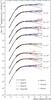 |
Fig. 9 TOA (modulated) fluxes (times |

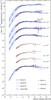 |
Fig. 10 Same as in Fig. 9, but the source spectra are now fitted on the CREAM-II data only (no published data for S, Ar, and Ca). |
Fit to CREAM-II and TRACER data.
Figure 10 shows the resulting best-fit spectra for the same models, but now fitted to CREAM-II data only. The data being at higher energy, the parameter ηS is unconstrained and we set it to −1 for this fit only. Not surprisingly, most models are not able to match the lower-energy HEAO-3 data. For the lighter species, α + δ remains the same, regardless of the model. The CREAM-II data for these species are ≳100 GeV/n, in a regime where the asymptotic slope γasympt is reached. For the heavier species, where the data extend down to a few tens of GeV/n, a similar ordering (though less clear) of the models with γasympt (as for the HEAO-3 fit) is seen for the high-energy asymptotic behaviour. The fits to TRACER data shown in Fig. 11 show an intermediate behaviour. Indeed, the energy range covers the same energy range as CREAM-II, but a few data point at low energy give a turn-over in the spectrum. However, there is a gap between the two energy regimes, where the curvature of the HEAO-3 data is not reproduced7.
Goodness of fit.
Table 4 shows the best-fit spectral
index αi and the associated
value for the various models, species,
and data sets. Unsurprisingly, the best-fit (smaller
value) are for the CREAM-II data that
only cover the high energy range. It is indeed more difficult to reproduce the low
energy part, where data have smaller error bars, but also where more effects
(modulation, continuous and catastrophic losses) shape the spectrum. For the
HEAO-3 case, the value is large for most of the species
because of the difficulty to fit the highest energy point that has a very small error
bar. For S, Ar and Ca, the fit is better. Data from the next CREAM flights, or from
the AMS-02 instrument should help clarify the situation, and confirm or otherwise
these discrepancies amongst the various data. Nevertheless, some conclusions can still
be drawn on the spectral indices (see below), although they are less constraining than
those derived from the p and He data.
Best-fit spectral index α and associated
for the fit of the source
spectrum parameters.
Confidence intervals on α, q and ηS.
Figure 12 shows, along with the 68% and
95% CIs, the best-fit values on the spectral
indices αi (top panel), the relative
source abundances qi (middle panel), and
the source parameter , for all the primary species
considered in this study. We first underline that the 95% CL relative uncertainty for
the parameters ranges from ≲5% on αi
and ≲20% on qi. CREAM data cover too
narrow an energy range to give stringent constraints, so we do not comment on them
further below. The following trends are observed for the parameters:
-
α (top panel): as for the p and He data, model II (reacceleration only, filled circle) always gives a larger value than the other models. Moreover, a similar range of slopes is found (2.2−2.5 for HEAO-3 data only, but more scatter when using TRACER data).
-
qi (middle panel): the relative abundances from HEAO-3 data are quite insensitive to the propagation model used. We recover the values of Engelmann et al. (1990) (green boxes), although with larger error bars. The Engelmann et al. (1990) analysis is based on the leaky-box model, so that their results are consistent with the Putze et al. (2009) analysis (yellow boxes) performed in the same framework. Similar results are obtained in the diffusion model (this analysis), except for the discrepancy for S, Ar and Ca (our values are larger than those of the HEAO-3 analysis). The difference for Ar and Ca may be related to the fact these elements were assumed to be pure primary species in this analysis (in order to speed up the calculation). The lack of the secondary contribution translates in a higher primary flux required to match the data. This underlines the importance of taking properly into account all nuclei to derive the source abundances. Part of the discrepancy could also be related to the fact that, for the S, Ar, and Ca elements, the highest energy data point is better fitted than for the others (see above): this results in a larger value of ηS and α that may be responsible for the difference observed on the qi. The relative abundances obtained from the TRACER data are sensitive to the model chosen, presumably because of the lack of constraints in the intermediate energy range. The relative abundances for model III (open squares) are consistent with those obtained from HEAO-3 data, whereas the obtained values for model II (filled circles) and III/II (open diamonds) systematically undershoot those from HEAO-3 data. If we look into Table 4, we remark that the fit to the Si data, on which all other abundances are normalised, is very poor for these models (large value of the
). The consistently low values
for all elements for these two models can be simply explained in terms of a too
large Si abundance obtained from the TRACER data for models II and III/II. The
fact that model III, which gives a good fit to Si data, gives abundances in
agreement with those derived from HEAO-3 data, supports this explaination. -
ηS (bottom panel): as for the p and He data, a trend is observed showing a dependence on the models. The pattern is the same, but with the value of ηS larger by one than that for p and He. In terms of ηS − ηT, the C to Si primary species favour a value ≈1, whereas p and He data favour ≈0. There is more scatter in the S to Fe data, but we note that the HEAO-3 data are based on different use of sub-detectors for this heavier species.
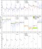 |
Fig. 12 Best-fit value (symbols), 68% (dashed error bars) and 95% (solid error bars) CIs for C to Fe source parameters from the fit on CREAM-II, HEAO-3, and TRACER data. Top panel: source spectral index αi. Middle panel: relative abundances qi. The results from the analysis of the HEAO-3 group (Engelmann et al. 1990) are shown as green boxes, and those from the TRACER group (Ave et al. 2009) as orange boxes. The yellow boxes correspond to a leaky-box analysis of the abundances on HEAO-3 data performed in Putze et al. (2009). Bottom panel: low-energy source parameter ηS (see Eq. (6)). Only the results from HEAO-3 data are plotted (for CREAM-II, ηS is set to −1, and for TRACER, the scatter is so large that the values are meaningless). |
4.4. Summary for the source parameters
An important result of the fixed transport parameter analysis is that, independent of the model and data considered, the source slope of p and He nuclei is constrained to fall in the range 2.2−2.5 (or 2.2−2.4 if we discard model II). As the range of δ covered by these models falls in the range 0.23−0.86 (see Table 2), this is a robust prediction. It also means that the asymptotic value for the propagated spectra (γasymp. ≡ α + δ), that falls in the range 2.7−3.0, is not reached in the GeV/n to TeV/n regime (as direct fits to the nuclei at Ek/n > 100 GeV/n propagated spectra lead to γdata ≈ 2.65, Ave et al. 2008): residual propagation effects (reacceleration, convection, spallations) are still active. This is also supported by the results on the heavier species.
Another important result is that regardless of the propagation model used, the quantity ηS − ηT is constrained to be ~0−1 for all primary nuclei considered. Hence, to reproduce the data, if a pure power-law rigidity spectrum is assumed, a non-standard low-energy diffusion coefficient (upturn at low energy) is required. Conversely, if a standard diffusion coefficient is assumed (i.e. K(E) = K0βℛδ), a flattening of the low-energy source spectrum is required (i.e. dQ/dR ∝ βηS+1ℛ−α with ηS > −1). The close-to-IS condition low-energy Voyager data is a further piece of information to break the degeneracy ηS − ηT, and would possibly provide the shape of the low-energy source spectrum.
Finally, most of the derived relative source abundances are in agreement with those derived by earlier groups. Still, a slight dependence on the propagation configuration is also observed. Due to the relevance of the value of the source abundances in the context of acceleration mechanisms (Dwyer & Meyer 1987; Meyer et al. 1997; Ellison et al. 1997; Ogliore et al. 2009), this point deserves further investigation.
5. Ratio of primary species
Webber & Lezniak (1974), more than 30 years ago, recognised the importance of looking at primary ratios. Such ratios may be, in principle, used to i) check the consistency of spectral indices of various species; ii) inspect whether source spectra are power-low in rigidity or power-law in kinetic energy; and also iii) inspect whether solar modulation is a rigidity or total energy effect. Below, we present several plots to illustrate some of these ideas, but also underline the complications that arise due to the many degeneracies between the source, transport, and modulation parameters (as underlined in the previous sections).
5.1. p/He ratio
Concerning the p/He ratio8 on which Webber & Lezniak (1974) study mainly focused, the main conclusions were: i) proton and helium source spectra are rigidity rather than energy/nucleon spectra; ii) modulation effects dominate the shape of the p/He ratio for such rigidity spectra when shown as a function of kinetic energy; and iii) modulation effects is not a pure rigidity effect since it flattens the spectrum at low energy relative to the interstellar flux.
p/He from the toy-model calculation.
Caution is in order when calculating the ratio p/He, whether we start from the
differential flux in energy or in rigidity. In an analogous manner as for Eq. (5), 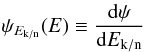 and
and 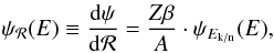 in order to define
 In the 1D toy-model (energy gains and
losses discarded), assuming Eq. (6) for
the source term – i.e.
dQ/dℛ = qβηS+1ℛ−α
–, and Eq. (3) for the diffusion
coefficient – i.e.
K(ℛ) = βηTK0ℛδ
–, we have the analog of Eq. (9), but
expressed in terms of the rigidity:
In the 1D toy-model (energy gains and
losses discarded), assuming Eq. (6) for
the source term – i.e.
dQ/dℛ = qβηS+1ℛ−α
–, and Eq. (3) for the diffusion
coefficient – i.e.
K(ℛ) = βηTK0ℛδ
–, we have the analog of Eq. (9), but
expressed in terms of the rigidity: 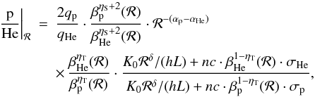 (11)where we made explicit the rigidity
dependence for all the terms (c is the speed of light). If the
destruction rate is subdominant, we have
(11)where we made explicit the rigidity
dependence for all the terms (c is the speed of light). If the
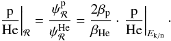
destruction rate is subdominant, we have 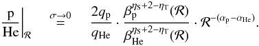 (12)In all the above formulae, we have
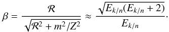 For a proton
m2/Z2 ≈ 1, whereas ≈4 for a
helium nucleus. This is sufficient to distort the low energy p/He ratio whenever it is
calculated from the differential fluxes in rigidity and
ηS + 2 − ηT ≠ 0. However,
if the ratio is calculated from the differential fluxes in kinetic energy per nucleon,
for a given Ek/n, we have
βp(Ek/n) ≈ βHe(Ek/n) ≡ β,
and Eq. (11) reduces to
For a proton
m2/Z2 ≈ 1, whereas ≈4 for a
helium nucleus. This is sufficient to distort the low energy p/He ratio whenever it is
calculated from the differential fluxes in rigidity and
ηS + 2 − ηT ≠ 0. However,
if the ratio is calculated from the differential fluxes in kinetic energy per nucleon,
for a given Ek/n, we have
βp(Ek/n) ≈ βHe(Ek/n) ≡ β,
and Eq. (11) reduces to ![Mathematical equation: \begin{eqnarray} \left.\frac{\rm p}{\rm He}\right|_{E_{\rm k/n}} &\approx & \frac{q_{\rm p}}{q_{\rm He}} \cdot \frac{[E_{\rm k/n}(E_{\rm k/n}+2)]^{-(\alpha_{\rm p}-\alpha_{\rm He})/2}}{2^{-\alpha_{\rm He}}} \nonumber\\ && \times \, \frac{K_0 [E_{\rm k/n}(E_{\rm k/n}+2)]^{\delta/2}2^\delta/(hL) + n c \beta^{1-\eta_{\rm T}} \sigma_{\rm He}}{ K_0 [E_{\rm k/n}(E_{\rm k/n}+2)]^{\delta/2}/(hL) + n c \beta^{1-\eta_{\rm T}} \sigma_{\rm p}}\cdot \label{eq:ekn} \end{eqnarray}](/articles/aa/full_html/2011/02/aa16064-10/aa16064-10-eq211.png) (13)When the destruction rates are subdominant,
we get
(13)When the destruction rates are subdominant,
we get ![Mathematical equation: \begin{equation} \left.\frac{\rm p}{\rm He}\right|_{E_{\rm k/n}} \stackrel{\sigma\rightarrow 0}{=} \frac{q_{\rm p}}{q_{\rm He}} \cdot \frac{[E_{\rm k/n}(E_{\rm k/n}+2)]^{-(\alpha_{\rm p}-\alpha_{\rm He})/2}}{2^{-\alpha_{\rm He}-\delta}}\cdot \label{eq:ekn_no_spall} \end{equation}](/articles/aa/full_html/2011/02/aa16064-10/aa16064-10-eq212.png) (14)
(14)
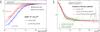 |
Fig. 13 Left panel: p/He ratio as a function of Ek/n, along with BESS98 (Sanuki et al. 2000) and BESS-TeV (Haino et al. 2004) data. The lines show the toy-model calculation without the destruction term (thick solid lines) and with it (thick dotted lines). The black, red and blue lines are respectively modulated to Φ = 0 MV (IS), Φ = 591 MV and Φ = 1109. Left panel: same ratio, but as a function of the rigidity. The data are AMS-01 (AMS Collaboration et al. 2002), ATIC (Zatsepin et al. 2003), CAPRICE 94 (Boezio et al. 1999), and some balloon data (Webber et al. 1987). The three toy-model calculations corresponds to the destruction rate set to zero (solid lines) or to its required value (dotted lines), plus a difference in the spectral index of p and He (dashed lines). In both plots, the normalisation is arbitrarily set to match the data. |
Comparison to data.
The p/He ratio is displayed as a function of the kinetic energy per nucleon in the left panel of Fig. 13, for the BESS98 (red squares) and BESS-TeV (blue circles) data. The solid lines (no inelastic reaction terms) result from Eq. (14), with αp = αHe. The shape of the ratio as well as the differences between the data taken at two different solar periods can be almost completely ascribed to the modulation effect. The effect of the inelastic reaction term is contained in Eq. (13). A closer look to this equation shows that the numerator and the denominator do not differ by a factor of more ~3, confirming the sub-dominant (though important) role of this effect in determining the ratio (displayed versus kinetic energy per nucleon). The effects (not shown) of having different spectral indices for p and He, having different values of α, δ, and ηS − ηT, when varied within reasonable limits, is of the same amount as the effect of the destruction rate. However, these effects are better seen when working with the rigidity.
The right panel of Fig. 13 shows a few experiments that have provided the p/He ratio as a function of the rigidity. Except for ATIC-1, the error bars were not provided by the experiments, but are expected to be of the order of the size of the symbols9. As underlined in the previous sections, even though all experiments claim small error bars, not many of them are consistent with each other for the p and He fluxes. On the other hand, one would expect the ratio to have less systematics than fluxes. Nevertheless, a large discrepancy remains, which cannot be explained by the different level of solar modulation associated to each experiment. The various curves show: i) the effect of solar modulation is sub-dominant for p/He vs. ℛ (thick vs. thin lines); ii) the effect of inelastic interactions, which are switched off (solid lines) or included (dotted lines); iii) the distortion of the p/He ratio due to a possible difference in the spectral indices of p and He (dashed lines). The shape of the ratio depends mostly on the value of ηS − ηT. As found in Eq. (12), the ratio is constant if ηS − ηT = −2 (not shown on the figure). The best-fit to the data is obtained for ηS − ηT ≈ 1, in general agreement with the results of the more complete analysis of Sect. 4.2. A small difference αp − αHe ≲ 0.05 between p and He source indices is not excluded. Note that the unperfect match to the data may result from the effect of energy losses which is not implemented in the toy formula.
5.2. Ratio relative to the oxygen flux
A similar analysis can be carried out for ratios of heavier species (Z > 2). In that case, for any element, we have A/Z ~ 2, so that for a given kinetic energy per nucleon, the rigidity or the β is the same for any element. The toy-model formulae is very similar to those for p/He Eq. (13): the parameters ηS and ηT, as well as the solar modulation effect are not expected to be important. This is shown in the top panel of Fig. 14, for a few elements: the main ingredient shaping the X/O ratios is the inelastic scattering on the ISM.
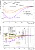 |
Fig. 14 Ratio of element to O as a function of the kinetic energy per nucleon. Top panel: C/O, Si/O and Fe/O without (IS, solid lines) or with (TOA, dashed lines) solar modulation. The destruction cross-section is indicated for each element. Bottom panel: comparison of the simple toy-model formula (thick solid lines) with the data (symbols): CREAM I and II (Ahn et al. 2008, 2009, 2010a,b), CRN (Swordy et al. 1990; Mueller et al. 1991), HEAO-3 (Engelmann et al. 1990), TRACER (Ave et al. 2008, 2009), and low-energy ACE data (George et al. 2009). |
There is a fair agreement with the data for C/O (black), Si/O (orange) and Fe/O (magenta) as shown on the bottom panel of Fig. 14, especially at low-energy with the ACE data (George et al. 2009). The discrepancy with Ne/O and Mg/O is only at the level of ~20%. This could be due to systematics in the data, but this deserves further investigation, especially because some isotopic anomalies in the Ne (and less likely for Mg) could be a signature for a contribution of the Wolf-Rayet stars to the standard cosmic-ray abundances (Gupta & Webber 1989; Webber et al. 1997; Binns et al. 2005, 2008), or related to acceleration in super-bubbles (e.g., Higdon & Lingenfelter 2003).
6. Conclusions
We have studied the spectra of proton, helium and other primary nuclei to derive the possible contraints and degeneracies on the source spectrum and the transport parameters. We have checked the compatibility of the primary fluxes with the transport parameters derived from the B/C analysis, and inspected whether they add further constraints. We have then derived the source parameters: slope of the power-law spectrum, abundance and low-energy shape.
In Sect. 3, we have analysed the fluxes of primary cosmic rays in diffusion models with particular attention to p and He. The most recent data on p and He are well reproduced by a purely diffusive model, described by power-law source spectrum, isotropic diffusion coefficient, spallative destructions and electromagnetic energy losses. This conclusion holds for single data sets but it is not reproduced in a combined data analysis (except for AMS01 and BESS98 proton data), due to the mean level of consistency among the different data collections. The inspection of low energy (≤ 100 GeV/n) p and He data indicates that the purely diffusive regime is likely not reached due to the role of spallations and, to less extent, of energy losses. The data are shown to be compatible with a wide class of purely diffusive models, but can also be accommodated by models with convection and/or acceleration. In all scenarios, they do not put significant constraints on the transport parameters and tend to favour values for the source and transport parameters outside reasonable physical limits.
In Sect. 4 we have applied best-fit models previously selected from B/C data, to the propagation of light and heavier primary nuclei, where we consider the possibility of low-energy deviations both in the diffusion coefficient K(R) = K0βηTℛδ and in the acceleration spectrum dQ/dR = qβηS+1ℛ−α. The main results on p and He are: i) it is possible to accommodate these primary fluxes in diffusive models along with B/C data (very good fit on BESS data, less satisfactory on AMS ones); ii) α ranges between 2.2 and 2.5; iii) for any given data set and species the spread in the source power index is αp − αHe ≲ 0.2, regardless of the model; iv) p and He point to very similar ηS, whose values depend on the model: close to 1 for the reacceleration and convection/reacceleration models, whereas ηS is close to −2 for model I/0 and −1.5 for model III/II, which contain a low energy upturn in the diffusion coefficient by means of ηT. Indeed, the constraint which seems to emerge from any propagation model is on their difference: ηS − ηT ≈ 0 − 1. We have demonstrated that a possible way to break the degeneracy ηS − ηT inherent the low-energy tail is by means of the Voyager data, taken at a few hundreds of MeV/n, and in a quasi-IS regime.
We have also studied heavier primary nuclei spectra, whose relevant destruction rate on the ISM increases roughly with atomic number. Therefore, they can be tested against a universal source spectral function. As for p and He, we have fitted data for C, O, Ne, Mg, Si, S, Ar, Ca and Fe using the models selected based on B/C. As for light primaries, these nuclei point to α around 2.2 − 2.5 regardless of the propagation configuration used. The quantity ηS − ηT is also constrained from C to Fe primary data to be ηS − ηT ≈ 1. Moreover, most of the derived relative source abundances are in agreement with those derived by earlier groups. We have shown that it is possible to reproduce the primary cosmic-ray spectra from protons to iron for all considered models (with or without convection/reacceleration) without a need for an artificial break in the injection slope at 10 GV, as it is assumed, e.g., in Trotta et al. (2010). This is also consistent with the leaky-box analysis of Putze et al. (2009).
In Sect. 5, we have studied the ratio of two primary species. The shape of the p/He ratios, when plotted as a function of the kinetic energy per nucleon, is driven by the modulation effect. This effect could be used to monitor the modulation level at different periods. On the other hand, the same ratio plotted as a function of the rigidity minimises the effect of the modulation, and is well adapted to probe the values of ηS − ηT, and αp − αHe. A full analysis using energy gains and losses is required to further develop such an approach, which is complementary to the direct fit of the p and He fluxes, and which may suffer less from systematics in the data. For X/O ratios, where X is an primary element with Z > 2, the behaviour as a function of Ek/n is driven by the destruction rate on the ISM. Isotopic anomalies and/or non-universality of the source slopes can be inspected by means of these ratios.
For the primary spectra and ratio of primary spectra, the importance of the destructive terms on the measured spectra has not previously been much considered. This is an innovation of the paper. We have also detailed the degeneracy between the source and propagation parameters, and provided probability density functions for the spectral index, abundance and low-energy shape of the source spectra for all species, as a means to address the question of the universality of the source spectra and their low-energy shape. Our analysis reinforces the need of more accurate data on light primary nuclei not only in the low-energy regime but also in the TeV/n-PeV/n range, as well as accurate measurement of primary-to-primary ratio. With such data it would be possible to significantly constrain the low-energy shape of the diffusion coefficient and the source spectrum, and fix the asymptotic behaviour of propagated nuclei.
Online material
Appendix A: Source slopes and relative elemental abundances
Most probable values and 68% CIs on the spectral index α and the relative source abundance qZ/qSi for the fit of the source spectrum parameters.
The isotopic separation is not always achieved, so that many data actually correspond to 1H+2H for the proton flux and 3He+4He for the helium flux, where 2H and 3He come from secondary contributions only. This amounts to a ≲ 10% error at low energy, which is contained in the error bars.
Throughout the paper, the quantity ψ denotes the differential flux in kinetic energy per nucleon, i.e. dψ/dEk/n. The notation dψ/dℛ used in Sect. 5 is the only place where it will refer to the differential flux in rigidity.
Putze et al. (2009) show that the values of the source-spectrum parameters (slope and abundances) are positively correlated among themselves and with the reacceleration strength, but are negatively correlated with the other propagation parameters.
The MCMC technique and the interface with the propagation code is explained in details in Putze et al. (2009). A shorter introduction is given in Putze et al. (2010).
We underline that for IS fluxes, the lowest energy data points are at ~0.8 GeV/n for p and ~0.4 GeV/n for He, see Fig. 2. This corresponds to βp ~ 0.8 (βHe ~ 0.7), so that having a pre-factor β3 amounts to a difference of ~1/2 (~1/3 for He) with respect to the case ηS = 0 for this low energy point.
The estimated modulation parameter is 60 MV for these data (Webber & Higbie 2009).
Model I/0 is not used on these data because it leads to unphysical values. This is likely to be related to the unphysical large negative value of ηS required, that becomes an issue for the numerical inversion of the energy losses (no convection and reacceleration to smooth out the steep upturn in the low-energy spectrum here, at variance with the three other models).
Note that because of the misidentification of 3He and 4He, Webber & Lezniak (1974) estimate a ≲ 2.5% effect in the data plotting the same measurement as rigidity spectra or kinetic energy spectra, that is also not considered below.
The AMS-01 p and He flux given in AMS Collaboration et al. (2002) are not calculated for the same rigidity binning. We thus fitted both fluxes (expressed as a function of the nucleus rigidity) with a simple polynomial function, and calculated the ratio from these fits (shown as stars approximately along the same binning as the original He data AMS Collaboration et al. 2000). Calculating correctly the associated error bars is not straightforward: as the data are just used for eye comparison, we do not go into more details. This difficulty in computing spectra binned in rigidity or kinetic energy suggests that in future experimenters should provide both.
Acknowledgments
We thank Alexander Panov for providing us an ASCII file of the ATIC data and Makoto Hareyama for providing us the RUNJOB and other experiment data points. D.M. thanks Laurent Derome and William Gillard for useful comments and discussions on the paper.
References
- Ahn, H. S., Allison, P. S., Bagliesi, M. G., et al. 2008, Astrop. Phys., 30, 133 [NASA ADS] [CrossRef] [Google Scholar]
- Ahn, H. S., Allison, P., Bagliesi, M. G., et al. 2009, ApJ, 707, 593 [Google Scholar]
- Ahn, H. S., Allison, P., Bagliesi, M. G., et al. 2010a, ApJ, 714, L89 [Google Scholar]
- Ahn, H. S., Allison, P. S., Bagliesi, M. G., et al. 2010b, ApJ, 715, 1400 [Google Scholar]
- Alcaraz, J., Alpat, B., Ambrosi, G., et al. 2000, Phys. Lett. B, 490, 27 [NASA ADS] [CrossRef] [Google Scholar]
- AMS Collaboration,Alcaraz, J., Alpat, B., et al. 2000, Phys. Lett. B, 494, 193 [NASA ADS] [CrossRef] [Google Scholar]
- AMS Collaboration,Aguilar, M., Alcaraz, J., et al. 2002, Phys. Rep., 366, 331 [NASA ADS] [CrossRef] [Google Scholar]
- Asakimori, K., Burnett, T. H., Cherry, M. L., et al. 1998, ApJ, 502, 278 [Google Scholar]
- Ave, M., Boyle, P. J., Gahbauer, F., et al. 2008, ApJ, 678, 262 [Google Scholar]
- Ave, M., Boyle, P. J., Höppner, C., Marshall, J., & Müller, D. 2009, ApJ, 697, 106 [NASA ADS] [CrossRef] [Google Scholar]
- Binns, W. R., Wiedenbeck, M. E., Arnould, M., et al. 2005, ApJ, 634, 351 [NASA ADS] [CrossRef] [Google Scholar]
- Binns, W. R., Wiedenbeck, M. E., Arnould, M., et al. 2008, New A Rev., 52, 427 [NASA ADS] [CrossRef] [Google Scholar]
- Boezio, M., Carlson, P., Francke, T., et al. 1999, ApJ, 518, 457 [NASA ADS] [CrossRef] [Google Scholar]
- Boezio, M., Bonvicini, V., Schiavon, P., et al. 2003, Astrop. Phys., 19, 583 [Google Scholar]
- Boulares, A. 1989, ApJ, 342, 807 [Google Scholar]
- Caprioli, D., Amato, E., & Blasi, P. 2010, Astrop. Phys., 33, 160 [Google Scholar]
- Delahaye, T., Lavalle, J., Lineros, R., Donato, F., & Fornengo, N. 2010, arXiv e-prints [Google Scholar]
- Derbina, V. A., Galkin, V. I., Hareyama, M., et al. 2005, ApJ, 628, L41 [Google Scholar]
- Diehl, E., Ellithorpe, D., Müller, D., & Swordy, S. P. 2003, Astrop. Phys., 18, 487 [Google Scholar]
- Donato, F., & Serpico, P. D. 2010, [arXiv:1010.5679] [Google Scholar]
- Donato, F., Maurin, D., Salati, P., et al. 2001, ApJ, 563, 172 [NASA ADS] [CrossRef] [Google Scholar]
- Donato, F., Maurin, D., & Taillet, R. 2002, A&A, 381, 539 [NASA ADS] [CrossRef] [EDP Sciences] [Google Scholar]
- Donato, F., Fornengo, N., & Maurin, D. 2008, Phys. Rev. D, 78, 043506 [NASA ADS] [CrossRef] [Google Scholar]
- Donato, F., Maurin, D., Brun, P., Delahaye, T., & Salati, P. 2009, Phys. Rev. Lett., 102, 071301 [Google Scholar]
- Drury, L. O. 1983, Rep. Prog. Phys., 46, 973 [NASA ADS] [CrossRef] [Google Scholar]
- Duvernois, M. A., & Thayer, M. R. 1996, ApJ, 465, 982 [Google Scholar]
- Dwyer, R., & Meyer, P. 1987, ApJ, 322, 981 [NASA ADS] [CrossRef] [Google Scholar]
- Ellison, D. C., Drury, L. O., & Meyer, J.-P. 1997, ApJ, 487, 197 [NASA ADS] [CrossRef] [Google Scholar]
- Engelmann, J. J., Ferrando, P., Soutoul, A., Goret, P., & Juliusson, E. 1990, A&A, 233, 96 [NASA ADS] [Google Scholar]
- Ferrand, G., & Marcowith, A. 2010, A&A, 510, A101 [NASA ADS] [CrossRef] [EDP Sciences] [Google Scholar]
- Ferrand, G., Downes, T., & Marcowith, A. 2008, MNRAS, 383, 41 [NASA ADS] [Google Scholar]
- George, J. S., Lave, K. A., Wiedenbeck, M. E., et al. 2009, ApJ, 698, 1666 [Google Scholar]
- Gilmore, G., Gustafsson, B., Edvardsson, B., & Nissen, P. E. 1992, Nature, 357, 379 [NASA ADS] [CrossRef] [Google Scholar]
- Gupta, M., & Webber, W. R. 1989, ApJ, 340, 1124 [NASA ADS] [CrossRef] [Google Scholar]
- Haino, S., Sanuki, T., Abe, K., et al. 2004, Phys. Lett. B, 594, 35 [NASA ADS] [CrossRef] [Google Scholar]
- Herbst, K., Kopp, A., Heber, B., et al. 2010, J. Geophys. Res. (Space Phys.), 115 [Google Scholar]
- Higdon, J. C., & Lingenfelter, R. E. 2003, ApJ, 590, 822 [NASA ADS] [CrossRef] [Google Scholar]
- Ichimura, M., Kogawa, M., Kuramata, S., et al. 1993, Phys. Rev. D, 48, 1949 [Google Scholar]
- Ivanenko, I. P., Shestoperov, V. Y., et al. 1993, ICRC, 2, 17 [Google Scholar]
- Jones, F. C. 1994, ApJS, 90, 561 [NASA ADS] [CrossRef] [Google Scholar]
- Jones, F. C., Lukasiak, A., Ptuskin, V., & Webber, W. 2001, ApJ, 547, 264 [NASA ADS] [CrossRef] [Google Scholar]
- Lavalle, J. 2010, arXiv e-prints [Google Scholar]
- Lemoine, M., Vangioni-Flam, E., & Casse, M. 1998, ApJ, 499, 735 [NASA ADS] [CrossRef] [Google Scholar]
- Lionetto, A. M., Morselli, A., & Zdravkovic, V. 2005, J. Cosmol. Astro-Part. Phys., 9, 10 [NASA ADS] [CrossRef] [Google Scholar]
- Maurin, D., Donato, F., Taillet, R., & Salati, P. 2001, ApJ, 555, 585 [NASA ADS] [CrossRef] [Google Scholar]
- Maurin, D., Taillet, R., & Donato, F. 2002, A&A, 394, 1039 [NASA ADS] [CrossRef] [EDP Sciences] [Google Scholar]
- Maurin, D., Putze, A., & Derome, L. 2010, A&A, 516, A67 [NASA ADS] [CrossRef] [EDP Sciences] [Google Scholar]
- Menn, W., Hof, M., Reimer, O., et al. 2000, ApJ, 533, 281 [NASA ADS] [CrossRef] [Google Scholar]
- Meyer, J.-P., Drury, L. O., & Ellison, D. C. 1997, ApJ, 487, 182 [NASA ADS] [CrossRef] [Google Scholar]
- Mueller, D., Swordy, S. P., Meyer, P., L’Heureux, J., & Grunsfeld, J. M. 1991, ApJ, 374, 356 [Google Scholar]
- Nath, B. B., & Biermann, P. L. 1994, MNRAS, 267, 447 [NASA ADS] [CrossRef] [Google Scholar]
- Ogliore, R. C., Stone, E. C., Leske, R. A., et al. 2009, ApJ, 695, 666 [NASA ADS] [CrossRef] [Google Scholar]
- Osborne, J. L., & Ptuskin, V. S. 1988, SvA Lett., 14, 132 [Google Scholar]
- Padovani, M., Galli, D., & Glassgold, A. E. 2009, A&A, 501, 619 [NASA ADS] [CrossRef] [EDP Sciences] [Google Scholar]
- Panov, A. D., Adams Jr., J. H.,Ahn, A. S., et al. 2009, Bull. Russian Academy Sci.: Phys., 73, 564 [Google Scholar]
- Perko, J. S. 1987, A&A, 184, 119 [NASA ADS] [Google Scholar]
- Ptuskin, V. S., Moskalenko, I. V., Jones, F. C., Strong, A. W., & Zirakashvili, V. N. 2006, ApJ, 642, 902 [NASA ADS] [CrossRef] [Google Scholar]
- Putze, A., Derome, L., Maurin, D., Perotto, L., & Taillet, R. 2009, A&A, 497, 991 [NASA ADS] [CrossRef] [EDP Sciences] [Google Scholar]
- Putze, A., Derome, L., & Maurin, D. 2010, A&A, 516, A66 [NASA ADS] [CrossRef] [EDP Sciences] [Google Scholar]
- Sanuki, T., Motoki, M., Matsumoto, H., et al. 2000, ApJ, 545, 1135 [NASA ADS] [CrossRef] [Google Scholar]
- Scherer, K., Fichtner, H., Ferreira, S. E. S., Büsching, I., & Potgieter, M. S. 2008, ApJ, 680, L105 [NASA ADS] [CrossRef] [Google Scholar]
- Seo, E. S., & Ptuskin, V. S. 1994, ApJ, 431, 705 [NASA ADS] [CrossRef] [Google Scholar]
- Shikaze, Y., Haino, S., Abe, K., et al. 2007, Astrop. Phys., 28, 154 [Google Scholar]
- Strong, A. W., Moskalenko, I. V., & Ptuskin, V. S. 2007, Ann. Rev. Nucl. Part. Sci., 57, 285 [NASA ADS] [CrossRef] [Google Scholar]
- Swordy, S. P., Mueller, D., Meyer, P., L’Heureux, J., & Grunsfeld, J. M. 1990, ApJ, 349, 625 [NASA ADS] [CrossRef] [Google Scholar]
- Trotta, R., Johannesson, G., Moskalenko, I. V., et al. 2010, ApJ, submitted [arXiv:1011.0037] [Google Scholar]
- Wang, J. Z., Seo, E. S., Anraku, K., et al. 2002, ApJ, 564, 244 [NASA ADS] [CrossRef] [Google Scholar]
- Webber, W. R. 1987, A&A, 179, 277 [NASA ADS] [Google Scholar]
- Webber, W. R. 1998, ApJ, 506, 329 [Google Scholar]
- Webber, W. R., & Lezniak, J. A. 1974, Ap&SS, 30, 361 [Google Scholar]
- Webber, W. R., & Higbie, P. R. 2009, J. Geophys. Res. (Space Phys.), 114, 2103 [Google Scholar]
- Webber, W. R., Golden, R. L., & Stephens, S. A. 1987, ICRC, 1, 325 [Google Scholar]
- Webber, W. R., Lukasiak, A., & McDonald, F. B. 1997, ApJ, 476, 766 [NASA ADS] [CrossRef] [Google Scholar]
- Webber, W. R., Soutoul, A., Kish, J. C., & Rockstroh, J. M. 2003, ApJS, 144, 153 [NASA ADS] [CrossRef] [Google Scholar]
- Webber, W. R., Cummings, A. C., McDonald, F. B., et al. 2008, J. Geophys. Res. (Space Phys.), 113, 10108 [NASA ADS] [CrossRef] [Google Scholar]
- Zatsepin, V. I., Zamchalova, E. A., et al. 1993, ICRC, 2, 13 [Google Scholar]
- Zatsepin, V. I., Adams, J. H., Ahn, H. S., et al. 2003, ICRC, 4, 1829 [NASA ADS] [Google Scholar]
All Tables
Best-fit transport parameters for various configurations of the diffusion model (fitted on B/C data).
Best-fit spectral index α and associated
for the fit of the source
spectrum parameters.
Most probable values and 68% CIs on the spectral index α and the relative source abundance qZ/qSi for the fit of the source spectrum parameters.
All Figures
|
Fig. 1 Demodulated p and He data ( |
| In the text | |
|
Fig. 2 Demodulated p (top panel) and He (bottom panel)
flux |
| In the text | |
|
Fig. 3 Surfaces of α + γ for the best-fit models in the plane K0 − δ (free parameters are α and qp) on AMS-01 proton data. The colour code (from light to darker shades) for the contours superimposed on top of each graph correspond to (α + γ) = {2.8, 2.9, 3.0, 3.1, 3.2}. |
| In the text | |
|
Fig. 4 Surfaces of |
| In the text | |
|
Fig. 5 Left panels: PDF of the source slope α for p (unfilled histograms) and He (hatched histograms). Right panels: PDF for αHe − αp. The colour code corresponds to the three experimental data used: AMS-01 (solid black line), BESS98 (dashed red lines) and BESS-TeV (dash-dotted lines). |
| In the text | |
|
Fig. 6 Most-likely value (symbols), 68% and 95% CIs for p (filled symbols) and He (open symbols) for the four propagation configurations gathered in Table 2. Top panel: spectral index α. Bottom panel: low-energy source parameter ηS (see Eq. (6)). The grey line ηS = −1 corresponds to the value for which the source spectrum is a pure power-law in rigidity (i.e. dQ/dℛ ∝ ℛ−α). |
| In the text | |
|
Fig. 7 TOA (modulated) fluxes (times |
| In the text | |
|
Fig. 8 95% CL envelopes for the proton and helium fluxes for the four propagation configurations of models of Table 2. The three panels correspond respectively to the result of the MCMC analysis on AMS-01 data (left panel), BESS98 data (middle panel), and BESS-TeV (right panel). For the sake of comparison, the IS (demodulated) AMS-01 (black circles), BESS98 (red squares), BESS-TeV (blue triangles), along with the Voyager data (stars). |
| In the text | |
|
Fig. 9 TOA (modulated) fluxes (times |
| In the text | |
|
Fig. 10 Same as in Fig. 9, but the source spectra are now fitted on the CREAM-II data only (no published data for S, Ar, and Ca). |
| In the text | |
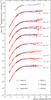 |
Fig. 11 Same as in Fig. 9, but the source spectra are now fitted on the TRACER data only. |
| In the text | |
|
Fig. 12 Best-fit value (symbols), 68% (dashed error bars) and 95% (solid error bars) CIs for C to Fe source parameters from the fit on CREAM-II, HEAO-3, and TRACER data. Top panel: source spectral index αi. Middle panel: relative abundances qi. The results from the analysis of the HEAO-3 group (Engelmann et al. 1990) are shown as green boxes, and those from the TRACER group (Ave et al. 2009) as orange boxes. The yellow boxes correspond to a leaky-box analysis of the abundances on HEAO-3 data performed in Putze et al. (2009). Bottom panel: low-energy source parameter ηS (see Eq. (6)). Only the results from HEAO-3 data are plotted (for CREAM-II, ηS is set to −1, and for TRACER, the scatter is so large that the values are meaningless). |
| In the text | |
|
Fig. 13 Left panel: p/He ratio as a function of Ek/n, along with BESS98 (Sanuki et al. 2000) and BESS-TeV (Haino et al. 2004) data. The lines show the toy-model calculation without the destruction term (thick solid lines) and with it (thick dotted lines). The black, red and blue lines are respectively modulated to Φ = 0 MV (IS), Φ = 591 MV and Φ = 1109. Left panel: same ratio, but as a function of the rigidity. The data are AMS-01 (AMS Collaboration et al. 2002), ATIC (Zatsepin et al. 2003), CAPRICE 94 (Boezio et al. 1999), and some balloon data (Webber et al. 1987). The three toy-model calculations corresponds to the destruction rate set to zero (solid lines) or to its required value (dotted lines), plus a difference in the spectral index of p and He (dashed lines). In both plots, the normalisation is arbitrarily set to match the data. |
| In the text | |
|
Fig. 14 Ratio of element to O as a function of the kinetic energy per nucleon. Top panel: C/O, Si/O and Fe/O without (IS, solid lines) or with (TOA, dashed lines) solar modulation. The destruction cross-section is indicated for each element. Bottom panel: comparison of the simple toy-model formula (thick solid lines) with the data (symbols): CREAM I and II (Ahn et al. 2008, 2009, 2010a,b), CRN (Swordy et al. 1990; Mueller et al. 1991), HEAO-3 (Engelmann et al. 1990), TRACER (Ave et al. 2008, 2009), and low-energy ACE data (George et al. 2009). |
| In the text | |
Current usage metrics show cumulative count of Article Views (full-text article views including HTML views, PDF and ePub downloads, according to the available data) and Abstracts Views on Vision4Press platform.
Data correspond to usage on the plateform after 2015. The current usage metrics is available 48-96 hours after online publication and is updated daily on week days.
Initial download of the metrics may take a while.