| Issue |
A&A
Volume 526, February 2011
|
|
|---|---|---|
| Article Number | A49 | |
| Number of page(s) | 28 | |
| Section | Catalogs and data | |
| DOI | https://doi.org/10.1051/0004-6361/201015752 | |
| Published online | 21 December 2010 | |
Spectral catalogue of bright gamma-ray bursts detected with the BeppoSAX/GRBM
1
Dipartimento di FisicaUniversità di Ferrara,
via Saragat 1,
44122
Ferrara,
Italy
e-mail: guidorzi@fe.infn.it
2
INAF-IASF Bologna,
via P. Gobetti 101,
40129
Bologna,
Italy
3
Istituto IS Calvi, Finale Emilia (MO),
Italy
4
Jeremiah Horrocks Institute for Astrophysics and Supercomputing,
University of Central Lancashire, Preston
PR1 2HE,
UK
Received:
14
September
2010
Accepted:
23
October
2010
Context. The emission process responsible for the so-called “prompt” emission of gamma-ray bursts is still unknown. A number of empirical models fitting the typical spectrum still lack a satisfactory interpretation. A few GRB spectral catalogues derived from past and present experiments are known in the literature and allow to tackle the issue of spectral properties of gamma-ray bursts on a statistical ground.
Aims. We extracted and studied the time-integrated photon spectra of the 200 brightest GRBs observed with the Gamma-Ray Burst Monitor which flew aboard the BeppoSAX mission (1996–2002) to provide an independent statistical characterisation of GRB spectra.
Methods. The spectra have a time-resolution of 128 s and consist of 240 energy channels covering the 40–700 keV energy band. The 200 brightest GRBs were selected from the complete catalogue of 1082 GRBs detected with the GRBM (Frontera et al. 2009), whose products are publicly available and can be browsed/retrieved using a dedicated web interface. The spectra were fit with three models: a simple power law, a cut-off power law or a Band model. We derived the sample distributions of the best-fitting spectral parameters and investigated possible correlations between them. For a few, typically very long GRBs, we also provide a loose (128-s) time-resolved spectroscopic analysis.
Results. The typical photon spectrum of a bright GRB consists of a low-energy index around 1.0 and a peak energy of the ν Fν spectrum Ep ≃ 240 keV in agreement with previous results on a sample of bright CGRO/BATSE bursts. Spectra of ~35% of GRBs can be fit with a power law with a photon index around 2, indicative of peak energies either close to or outside the GRBM energy boundaries. We confirm the correlation between Ep and fluence, in agreement with previous results, with a logarithmic dispersion of 0.13 around the power law with index 0.21 ± 0.06. This is shallower than its analogous in the GRB rest-frame, the Amati relation, between the intrinsic peak energy and the isotropic-equivalent released energy (slope of ~0.5). The reason for this difference mainly lies in the instrumental selection effect connected with the finite energy range of the GRBM particularly at low energies.
Conclusions. We confirm the statistical properties of the low-energy index and peak energy distributions found by other experiments. These properties are not yet systematically explained in the current literature with the proposed emission processes. The capability of measuring time-resolved spectra over a broadband energy range, ensuring precise measurements of parameters such as Ep, will be of key importance for future experiments.
Key words: gamma-ray burst: general
© ESO, 2010
1. Introduction
Giant leaps in the knowledge of the gamma-ray burst (GRB) explosions have been made in the past 15 years, mainly thanks to the discoveries obtained by former BeppoSAX (1996–2002), HETE–II (2000–2006), and the current Swift (2004) and Fermi (2008) missions, as well as those made by ground facilities in response to the spacecraft triggers.
Time-integrated photon spectra of long GRBs can be adequately fit with a smoothly broken power law (Band et al. 1993), whose low-energy and high-energy photon indices, α and β, have median values of −1 and −2.3, respectively (Preece et al. 2000; Kaneko et al. 2006, hereafter K06). Similar results were obtained by time-resolved spectral analysis (Frontera et al. 2000; Ghirlanda et al. 2002; K06). In spite of this, the nature and emission mechanisms responsible for the prompt emission of GRBs are still a matter of debate.
The corresponding νFν spectrum peaks at Ep, the so-called peak energy, whose rest-frame value is found to correlate with other relevant observed intrinsic properties, such as the isotropic-equivalent radiated γ-ray energy, Eiso (Amati et al. 2002), or its collimation-corrected value, Eγ (Ghirlanda et al. 2004). These correlations are observed to hold statistically on the sample of GRBs with known intrinsic quantities; however, they are affected by a significant dispersion, which could be due to some hidden variables. Specifically, while the scatter of the Ep–Eiso relation is measured well and known to differ from zero (e.g., Amati et al. 2009), the same issue for the corresponding collimation-corrected relation is debated (e.g., Campana et al. 2007; Ghirlanda et al. 2007; McBreen et al. 2010). In the BATSE catalogue (Paciesas et al. 1999), the Ep distribution clusters around 300 keV with a ~100 keV width (K06).
From the phenomenological perspective, much effort has been made to characterise and identify typical spectral properties of bursts by applying parametric spectral models that characterise the most relevant quantities within the observational energy window. These quantities include the peak energy and the low and high energy components, which are related to the particle energy distribution and/or to the physical parameters of the emitting region, according to the most accredited emission theories.
One of the most promising mechanisms proposed for gamma-ray emission is the synchrotron shock model (SSM). This model assumes that the electrons in an optically thin environment are accelerated by the first-order Fermi mechanism to a power law distribution dN(γ)/dγ ∝ γ−p, where γ is the Lorentz factor. This distribution does not evolve in time, and the electron index p is related to the high-energy photon index either as β = −(p + 2)/2 for the fast-cooling synchrotron spectrum, or as β = −(p + 1)/2 for non-cooling synchrotron (Sari et al. 1998). The peak energy can be expressed as  , where
  is the pre-shock equilibrium electron energy and Bps the post-shock magnetic field (Tavani 1996).
The use of large catalogues represents a fruitful approach to studying the spectral properties of GRBs on statistical grounds. In particular, characterising the time-averaged photon spectra is important because it offers clues for understanding the radiation and particle acceleration mechanism at work during the prompt phase of GRBs, on which there is no consensus yet. In this paper, we extracted and studied the time-integrated photon spectra of the 200 brightest GRBs observed with the gamma-ray burst monitor (GRBM, Feroci et al. 1997; Frontera et al. 1997) aboard the BeppoSAX mission (Boella et al. 1997) and performed a novel statistical study of the main parameters characterising the GRB spectra.
The paper is organised as follows. Sections 2 and 3 report the observations, data reduction, and analysis. We report our results in Sect. 4, in the light of the models proposed in the literature, and Sect. 5 presents our discussion and conclusions.
All quoted errors are given at 90% confidence level for one interesting parameter (Δχ2 = 2.706), unless stated otherwise.
2. Observations
The GRB sample used for this analysis was extracted from the GRB catalogue of the BeppoSAX/GRBM (Frontera et al. 2009, hereafter, F09). The main constraints in the selection process were the following:
-
sufficient number of total counts on the most illuminated detector unit;
-
well-defined response function, connected with the information on the GRB arrival direction;
-
reliable background interpolation.
A number of GRBs (28) have also been detected in common with BATSE, whose data were published by K06 (see Sect. 4.8). For these bursts, in addition to exploiting the information on the GRB position derived by BATSE, which is useful for choosing the appropriate response function, we compared the results we obtained with the GRBM data with data in K06.
The background interpolation and subtraction required the availability of spectra acquired within contiguous time intervals around those that include the burst. This requirement limited the final number of selected events further.
Finally we ended up with 185 bright GRBs out of the 1082 GRBs belonging to the GRBM catalogue (F09). Hereafter, fluence Φ refers to the 40–700 keV energy band, unless otherwise specified. The values of the largest and lowest fluences included in the final sample are 1.7 × 10⁻⁴ and 4.4 × 10⁻⁶ erg cm-2.
3. Data reduction and analysis
Firstly, among the 128-s time intervals continuously sampled with a time-integrated spectrum, we identified those that include the GRBs and those that are adjacent, required for the background estimate. In some cases we took only the most illuminated unit for each GRB. In the remaining cases, we considered the two most illuminated units, apart from a few cases, for which it was possible to extract meaningful spectra from three different units. The two-unit case typically occurred when the burst direction with respect to the BeppoSAX local frame was such as to give comparable counts to both units. Data from the second most illuminated unit were ignored when the signal-to-noise (S/N) did not allow a statistically significant spectral reconstruction.
Table 1 reports the details of the data available for each analysed burst. For each spectrum the corresponding time interval refers to the on-ground trigger time (F09), expressed as seconds of day (SOD). Each spectrum of a given burst is tagged with a letter, and the corresponding packet number inherited from the GRBM archival data (and used in the GRB catalogue web interface1) is also reported.
The GRB spectra reduction and analysis is performed as
-
dead-time correction of both source and background 128-s long spectra (Sect. 3.1);
-
background fitting by interpolation of adjacent 128-s dead-time corrected spectra (Sect. 3.2);
-
identification of the appropriate GRBM response function (dependent on the GRB position; Sect. 3.3);
-
spectral fitting of background-subtracted GRB spectra:
-
GRB total spectrum (“time-integrated” spectrum);
-
individual 128-s spectra of the GRBs that happened to be split into two or more intervals (“time-resolved” spectra).
-
3.1. Dead-time correction
We set up the following procedure to correct the 128-s integrated spectra for dead time. The 40–700 keV light curve of the corresponding unit is taken into account because a nearly constant rate gives rise to a dead time effect below a rate with prominent peaks of short time duration. For a given average 128 s spectrum, let  be the observed counts in the 40–700 keV band for the ith 1-s bin (i = 1,...,128). The dead-time corrected counts, ci are calculated as
  , where τ = 4 μs is the dead time. Let fi be the rate fraction of the corresponding bin, defined as fi = ci/c, where c is the sum of all ci’s (i = 1,...,128). Let
  be the total number of measured counts in the 128-s spectrum integrated over the 240 energy channels, which must also satisfy
  (1)where s is the number of the total corrected counts we would have observed when integrating the spectrum in the absence of dead time. Therefore s can be estimated as the root of the equation
  (2)Assuming a negligible distortion of the original spectral shape due to dead time (which is the case when no strong spectral evolution occurs during the 128-s interval over which the spectrum is integrated), we renormalise the observed counts of each energy channel by the factor
  .
.
3.2. Background subtraction
To reliably estimate the background counts in each energy channel of the time-integrated spectra, and to ensure a safe interpolation, we made sure that spectra accumulated over 128-s time intervals temporally contiguous to the one that includes the burst, were also available. In a few cases, either the time interval preceding or the one following the GRB was not available, so in these cases, we checked that the background was stable enough (typically within a few %) to ensure linear (back)-extrapolation. For this reason we did not use the 128-s taken right before the ingress or right after the exit of a passage over the South Atlantic Anomaly.
 |
Fig. 1 1-s light curve of GRB 000226 detected with GRBM unit 2 in the 40–700 keV band shown as an example. The dashed horizontal line shows the parabolic fit to the background. The vertical lines mark the time intervals corresponding to the 128-s spectra continuously acquired. Spectra “A” and “B” include the GRB, while the adjacent intervals are used to interpolate the background in each channel. |
Figure 1 shows the example of GRB 000226 (#137 in Table 1). The independent spectral sampling happened to split this burst in two different 128-s spectra, called “A” and “B”, respectively. The light curve shown is the 40–700 keV profile of the most illuminated unit (GRBM 2): the background was interpolated with a parabolic fit (as in general), although a linear fit was already satisfactory. We identified the packet numbers corresponding to “A” and “B”: 30 and 31, respectively. We also took two couples of adjacent spectra preceding (28, 29) and following (32, 33) the burst spectra. All these spectra were dead-time corrected as in Sect. 3.1.
At this point we performed two operations closely connected with each other: background fitting and energy channels’ grouping. The latter operation is the result of ensuring a minimum significance (3σ) on the net counts of the final background-subtracted grouped energy channel. More in detail, this is how the procedure works: it extracts the light curve of a given (original) energy channel out of the selected spectra. This light curve is then fit linearly (excluding the spectra including the GRB) so that the interpolated background counts expected during the GRB intervals are estimated. These steps are repeated for a sequence of adjacent energy channels: every time an original energy channel is summed up, the light curve extraction and fitting is reiterated for the grouped energy channel, until the total net counts exceed the significance threshold. When this is the case, the used energy channels are grouped into a final single channel. An example of this is displayed in Fig. 2 for the same burst shown in Fig. 1: the light curve of energy channel 60 (in this case corresponding to the energy range 160–163 keV) is built up from 6 contiguous 128-s time intervals. A satisfactory linear fit is performed on the background intervals: the resulting net counts in the GRB intervals (“A” and “B”) match the significance requirement so that this channel can stand alone.
 |
Fig. 2 128-s light curve of energy channel 60 (160–163 keV) of GRB 000226 as seen with GRBM unit 2 (same example as in Fig. 1). The dashed line shows the linear fit of the background. Same vertical lines as in Fig. 1. |
The above steps are repeated until the full range of energy channels is covered. The last grouped channel, that in general does not fulfil the significance requirement, is merged into the previous one. The goodness of the fit of the background light curve for each grouped energy channel is expressed in terms of reduced χ2. This is then checked by the human operator to make sure that all the fits are acceptable. The uncertainty on the net counts of each grouped channel is calculated by propagating the statistical uncertainties of counts and those affecting the interpolated background.
All this applies to the meaningful channels, i.e. from 18 to 240 out of the 256 nominal channels, while the rest are ignored.
3.3. Response matrices
The knowledge of the appropriate response matrices for a given burst requires the GRB position with respect to the BeppoSAX reference frame to be known, also called “local” position. The reason is the complex dependence of the response function on the local direction and photon energy, due to the BeppoSAX payload itself surrounding the GRBM units. The GRBM response function for a generic direction was determined with Monte Carlo techniques (Calura et al. 2000) and in-flight calibrated with Crab observations and cross-calibrated with BATSE through commonly detected GRBs. See F09 for a detailed description.
Log of the 128-s energy spectra of the brightest GRBM bursts.
The information on the directions of the GRBs considered in this work was taken from F09, and the column “CAT” in Table 2 reports the ID of the catalogue providing the most accurate position of each GRB using the same convention as in F09. For those GRBs for which no such information is available, typically the GRBs detected by the GRBM alone and for which the localisation procedure did not give a unique, acceptable solution, we used as many response matrices as the possible directions and made sure that the spectral results were not significantly different from each other.
3.4. GRB spectra and models
For the GRBs whose profiles were sampled by multiple 128-s intervals, we extracted and fit both the total (time-integrated) and the individual (time-resolved) spectra. Whenever the burst was contained within a single interval, no time-resolved spectrum was possible. We adopted three possible fitting models: i) Band’s model (band; Band et al. 1993), ii) the cut-off power law (cpl), where the photon spectrum is N(E) ∝ E−α exp [−E (2 − α)/Ep] , and iii) a simple power law (pow), N(E) ∝ E−α.
In addition to the normalisation, the free parameters of the fitting models were the power law indices (the low- and high-energy α and β for band, only the low-energy index for the other models) and the peak energy, Ep, of the νFν spectrum. We note that the signs of the band photon indices follow a different convention from the other models. Spectral fitting was done using XSPEC v12.5 (Arnaud 1996).
Table 2 reports the spectral fitting results for the total spectra of all the bursts for various models. The pow model was adopted when the goodness of the fit, expressed through the reduced χ2, was already acceptable, and fitting the other models did not provide any useful constraint on Ep. This was typically the case for bursts with the Ep either above or below the energy passband of the GRBM and/or for spectra with relatively poor S/N. Following Sakamoto et al. (2008a), for each of the 185 time-integrated spectra we first fit each spectrum with each of the three models. Whenever passing from a model to a more complex one the total χ2 decreased by more than 6 for each additional degree of freedom, we considered it a significant improvement in modelling the spectrum (see Sakamoto et al. 2008a).
In most cases, the high-energy photon index β of the band function could not be constrained by the data, owing to the narrower energy passband of the GRBM compared with that of BATSE, as well as to the S/N of the spectra. In such cases, we fixed its value to the average value of −2.3 found on the BATSE sample (K06). In a few cases, the same problem occurred at low energies, for which we fixed the corresponding index α to the analogous value of −1.0.
We have not achieved a statistical improvement with the band model in any case except for three cases of time-resolved spectra, characterised by a high S/N (spectra B of 980615B, 971208B, and 970831). The best-fit model of each GRB is marked with an asterisk in Tables 2 and 3.
We excluded those bursts whose spectra gave a poor fit from statistical analysis, i.e. whose results in terms of χ2/d.o.f. can be rejected at 99% confidence level. These cases represent less than 3% of the total sample and are the following bursts: 980203B, 990118A, 000328, 001213, and 001228.
4. Results
4.1. Results in the BeppoSAX local frame
We studied the goodness of the spectral fit for each GRB as a function of the direction as referred to the BeppoSAX local frame of reference (F09). The aim is to check the goodness of the response matrix as a function of the GRB arrival direction. To this aim, we investigated how the total reduced χ2 for each GRB best-fitting spectral model depends on both the local azimuth φ, measured counterclockwise from the axis of GRBM unit 2, and the local altitude θ above the BeppoSAX equatorial plane.
 |
Fig. 3 Goodness of the fit for all the brightest GRBs with known arrival direction (143 out of 200) as a function of the BeppoSAX local azimuth angle φ. Vertical dashed lines at φ = 0°,90°,180°,270° correspond to the axes of GRBM units 2, 3, 4, 1, respectively. Empty squares (filled circles) are the GRBs localised by other experiments (GRBM alone), as reported in F09. |
Figure 3 shows the reduced χ2 of the best-fitting spectral model for each GRB as a function of the local azimuthal angle φ for 143 GRBs with known arrival direction out of our sample. The points are divided in two classes: those localised by other experiments, whose information on the direction is independent of the GRBM, and the remaining ones localised with the GRBM (see F09). Clearly both classes do not show any strong dependence of the goodness of the fit on the local azimuthal direction. We just note that GRBs close to GRBM unit 2 axis have slightly more scattered χ2 values than other units.
Figure 4 shows the goodness of the fit as a function of the local elevation or altitude angle θ. As for the azimuthal angle, the goodness of the fit shows no dependence on the elevation angle either. Noteworthy here is the presence of more GRBs (60% of the total) in the BeppoSAX northern hemisphere (θ > 0°): this is explained by the more effective absorption for southern directions due to the on-board electronics boxes in the lower part of the spacecraft (Guidorzi 2002), as shown by the number of bright GRBs, which drops significantly for elevation angles below −20°/−30°. The paucity of GRBM-localised GRBs compared with those localised by other instruments at directions close to the BeppoSAX local poles comes from the limitations of the GRBM localisation technique (F09).
4.2. Results of the POW model
The power law model (pow) provides acceptable fits for ~35% of the sample. This model represents the best-fitting model for 10% of the 100 brightest GRBs, and the same fraction rises to 53% when we consider the less bright half of the sample. The power law index αpow distribution was derived by selecting only those GRBs whose spectral fitting gave an uncertainty below 0.3. This choice was the result of a trade-off between the need for reasonably accurate values and the need for good statistics. As a consequence the sample shrank to 87%.
Spectral fitting results of the time-integrated spectra for each bright GRB. Frozen values are reported among square brackets.
Spectral fitting results of the time-resolved spectra for each bright GRB that were sampled by more 128-s time intervals.
 |
Fig. 4 Same as Fig. 3. Angle θ is the BeppoSAX local altitude above the equatorial plane, marked by the vertical dashed line. |
The resulting distribution of αpow can be fit with a Gaussian with  and σ(αpow) = 0.32 (top panel of Fig. 5), in agreement within the analogous results obtained over a sample by Swift/BAT (1.6 ± 0.2, Sakamoto et al. 2008a), as well over a sample of INTEGRAL (1.6 in the energy band 18–300 keV, Vianello et al. 2009). The slightly softer average value we obtained with the GRBM bursts is explained by the harder energy range considered, thus more likely to be affected by the steepening of the spectrum due to the high-energy component; this conclusion is also supported by the corresponding value (
 ) obtained over the BATSE sample (K06).
The softness of most spectra fit with a pow model is explained with most GRBs having Ep below ~100 keV. About 30% of the pow indices lie in the range 1.7 < αpow < 2.0, so their peak energies are likely to lie close to the upper bound or above it, i.e. Ep ≳ 700 keV. Another 37% of the same sample have αpow > 2 and their peak energies lie at Ep < 40 keV, as expected for the X-ray flashes (XRFs, Heise et al. 2001; Barraud et al. 2003; Sakamoto et al. 2005, 2008b; Pelangeon et al. 2008).
 |
Fig. 5 Top panel: αpow distribution for 55 GRBs with relative uncertainties smaller than 0.3. Mid panel: αcpl distribution for 77 GRBs with relative uncertainties smaller than 0.5. Bottom panel: alternatively to the cpl model, we show the −αband distribution for 31 GRBs for which the band function provides an acceptable fit, although not significantly better than the cpl. The vertical dotted and dashed lines show the cases α = 2/3 (synchrotron death line) and α = 3/2 (cooling death line). In each panel dashed distributions show the corresponding best-fitting Gaussian functions. |
4.3. Results of the CPL model
Similar to the pow model case, the distribution of the power law index for the cpl model was derived by selecting the GRBs with an uncertainty on αcpl smaller than 0.5. 77% of the sample passed this criterion. The resulting distribution is fit with a Gaussian with mean and standard deviation values of  and σ(αcpl) = 0.28 (mid panel of Fig. 5). Similar values were obtained from the observations of BAT on-board Swift: αcpl = 1.12 ± 0.15 (Cabrera et al. 2007), HETE-II: αcpl = 1.2 ± 0.5 (Barraud et al. 2003). There are no cases in which the low-energy index is very soft (α ≥ 2).
In the past, spectral fitting of time-resolved BATSE spectra of bright GRBs has yielded a significant number of cases with low-energy photon indices α below 2/3. This result is inconsistent with the SSM, and α = 2/3 has been referred to as its “death line” (Preece et al. 1998; Papathanassiou 1999, and references therein). Our results indicate that about 30% of them lie below the synchrotron death line of α = 2/3 (Fig. 5). On the other side of the distribution, no GRB lie beyond the fast-cooling death line (Ghisellini et al. 2000) represented by the limit α < 3/2.
Figure 6 shows the Ep distribution for the cpl model. Only values with uncertainties below 40% are displayed, and they represent 90% of the overall set of GRBs best fit with cpl. The distribution can be fit with a lognormal with mean and standard deviation of log Ep = 2.38 ± 0.18 (corresponding to a mode of Ep = 240 keV), fully consistent with the results obtained over a sample of bright BATSE bursts by K06. They found  keV using different fitting models.
 |
Fig. 6 Peak energy distribution derived with the cpl model for a sample of 106 GRBs with a relative uncertainty smaller than 40%. The dashed line shows the best-fitting normal distribution. |
Comparing the Ep distribution of our sample with the analogue of the BATSE GRBs fit only with the cpl model ( keV), although formally consistent with one another, suggests that the GRBM distribution is shifted towards lower values: this is primarily explained by the BATSE sensitivity at energies >700 keV. The consequence of this selection effect is that a number of bright GRBs detected with the GRBM and with Ep ≳ 700 keV are clearly missing in the observed Ep distribution of Fig. 6, and belong to the GRBs that were fit with a power law with αpow < 2.
We do not observe a sizable fraction of GRBs with Ep < 100 keV because our sample collects the brightest end of the GRBM fluence distribution: as a consequence, our sample is biased towards GRBs with high Ep values, because of its correlation with the fluence (Fig. 10).
 |
Fig. 7 Low-energy photon index vs. peak energy as determined with the cpl model on a sample of 70 GRBs with relatively accurate measurements. |
We analysed the possible relation (if any) between αcpl and Ep for a sample of 70 GRBs with both measurements sufficiently accurate by adopting the same thresholds mentioned above (0.5 on αcpl and 40% on Ep). Figure 7 shows this sample in the αcpl–Ep plane. A statistical study of our data shows no clear evidence of a correlation between these two quantities. In fact, the Spearman rank-order correlation coefficient over the whole sample turned out to be rs = −0.15 with an associated probability of 21% of no correlation. However, for the low peak energy subsample (log Ep/keV < 2.4) the probability drops to 0.6% (rs = −0.49), suggesting that the softer the peak energy, the softer the photon index. This type of correlation is expected because of the instrumental effect coming into play whenever Ep lies close to the edge of the energy passband. When this is the case, the low-energy photon index α as derived from the fitting procedure may not have reached the asymptotic value, thus resulting in a softer value (Preece et al. 1998; Lloyd & Petrosian 2000, 2002; Amati et al. 2002). This is indeed what we observe in Fig. 7. That such a correlation seems to become significant when considering only the GRBs with low Ep values is a clear indication of its instrumental origin.
The number of GRBs whose α estimates are biased because of this effect depends on how smoothly the spectrum reaches its asymptotic value, in addition to the energy window of the detector. The same problem also affects samples of GRB spectra obtained with different detectors. To circumvent this issue, in the case of BATSE GRBs Preece et al. (1998) defined the “effective low-energy photon index” as the tangential slope at 25 keV (lower energy bound of BATSE detectors) of the spectrum on a logarithmic scale. However, also with this definition the problem still remains whenever 25 keV is not low enough to reach the asymptote (Lloyd & Petrosian 2000). In our case, the impact on the α distribution shown in Fig. 5 is such that a few GRBs with 1.3 ≲ αcpl ≲ 1.5 are likely to suffer from this effect. Different detectors with different energy windows should also be affected differently. However, as noted above, the analogous distributions of other detectors, described by similar modes and dispersions, suggest that the impact of this instrumental effect on the observed α distribution is minimal.
4.4. Results of the BAND model
In none of the time-integrated spectra of our sample have we found a significant improvement when changing the fitting model from cpl to band. Nevertheless, to explore how the choice of either model may affect the result, in the bottom panel of Fig. 5 we show the −αband distribution for 31 GRBs for which the band function gave an acceptable result, although not significantly better than the cpl. Clearly, the two distributions are fully compatible with each other. In Sect. 4.7 we explore the relation between the use of the two models with our data in more detail.
4.4.1. High–energy index
For a subsample of 17 GRBs out of the 31 mentioned above, it was also possible to constrain the high-energy photon index β with absolute uncertainties smaller than 1. The distribution is shown in Fig. 8. The small number of events for which this estimate was possible is explained by the relatively small upper bound of the GRBM passband compared with that of BATSE. However, we note that the resulting distribution is fully compatible with what is derived on a more numerous BATSE sample (K06).
 |
Fig. 8 High-energy photon index β distribution of the band function for a sample of 17 GRBs. |
4.5. Fluence distribution
To account for the uncertainties in the response matrix calibration, we added a systematic 10% error in quadrature to the statistical fluence errors (F09). For each GRB we considered the fluence yielded by the corresponding best-fitting model. For the analysis we considered the mean value and symmetric error of the corresponding logarithms. The distributions of the best-fitting parameters and of the fluence were derived by excluding the GRBs affected by a relative uncertainty over 20% (after including the systematics); 12% of the sample were rejected as a consequence.
Figure 9 displays the cumulative fluence distribution compared with the corresponding distribution for 795 GRBs of the GRBM catalogue by F09, whose values were calculated through the 2-energy channel spectra (see Fig. 8 of F09). The observed distribution deviates from the power law distribution with index −3/2, predicted in the case of no luminosity function evolution with redshift and where the observed GRBs are homogeneously distributed in the sampled volume of an Euclidean space. The difference between the observed and the predicted −3/2 power law distributions had already been found in the BATSE catalogue (Meegan et al. 1992) and confirmed with the GRBM data (F09).
 |
Fig. 9 Cumulative fluence distribution for the subset of GRBs with a relative error on fluence below 20% (shaded histogram). The dashed histogram is the corresponding fluence distribution published by F09 for the entire GRBM catalogue of GRBs, as derived from 2-channel spectra. The solid line shows the power law distribution with index −3/2 expected if GRBs were homogeneously distributed in an Euclidean space throughout the sampled volume. |
4.6. Peak energy-fluence correlation
Figure 10 displays the observed peak energy Ep vs. fluence Φ for a sample of 108 bright GRBs with well determined values. The correlation is significant: the Spearman rank coefficient is rs = 0.48 with an associated chance probability of 1.4 × 10⁻⁷. Given the apparent scatter, we performed a power law fit by adopting the D’Agostini method (e.g., Guidorzi et al. 2006) and found the following best-fitting relation: 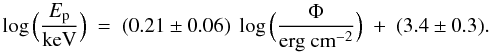 (3)The extrinsic scatter, which combines the intrinsic scatter due to the uncertainties of the individual points and must not be confused with it, is σlog Ep = 0.13 ± 0.02. The slope of the correlation agrees with previous values obtained on samples of BATSE GRBs (e.g. Lloyd et al. 2000; Nava et al. 2008). The scatter of each point in the Ep–Φ plane around the best-fit correlation is the result of the two sources of scatter: (i) the intrinsic, different for each point and accounting for the uncertainties in the evaluation process of both observables, and (ii) the extrinsic scatter, reflecting a property of the correlation itself through some unknown variables. The combination of the two scatter sources finally gives a normal distribution, as shown by the inset of Fig. 10; indeed, the normalised scatter ζi, defined by Eq. (4) with i running over the set of points, distributes according to a standardised Gaussian,
  (4)where yi = log Ep,i, xi = log Φi, with the ith σ the corresponding (intrinsic) uncertainties and σy the extrinsic one. m and q are the best-fit slope and constant values reported in Eq. (3), respectively.
 |
Fig. 10 Correlation between Ep and the 40–700 keV fluence for a sample of 108 bright GRBs with well determined values. The dashed line shows the best-fitting power law, with index 0.21 ± 0.06, while the dotted lines include the 1-σ region, where σ = 0.13 is the extrinsic scatter. Inset: distribution of the normalised scatter. The dashed line shows the standardised normal distribution. |
 |
Fig. 11 Peak energy determined with the cpl vs. the same determined with the band function for a sample of 63 GRBs with both measurements. The dashed and dotted lines show the equality and the best-fitting power law relations, respectively. In particular, according to the latter, the peak energy determined with the cpl tends to be ~20% higher than that of the band. |
It is known that truncation effects connected with the finiteness of the detector energy window may affect the distribution of the fitting parameters and the corresponding correlations. In particular, both Ep and fluence Φ suffer from them, as proven for BATSE GRBs by Lloyd et al. (2000), who investigated their impact in this respect. Our sample includes bright bursts, so truncation effects against low-fluence GRBs or near the detector threshold can be neglected. As discussed in Sect. 4.3, Ep is more likely to suffer from biases against low and high values (Lloyd & Petrosian 1999). Lloyd et al. (2000) tackled the issue of accounting for data truncation effects in the correlation studies by means of non-parametric techniques, which take the limits imposed by the detector in the determination of each parameter into account. Specifically for the Ep–Φ relation, they found similar results with these techniques that, when considering the bright subsample of BATSE bursts, are less affected than the GRBs close to the detector threshold. In both cases the value of the best-fitting slope (0.29 ± 0.03 and 0.28 ± 0.04, respectively) is similar to what is found on our set. This suggests that the slope of the Ep–Φ correlation for the bright end of the GRBs detected with the GRBM is only marginally affected by this kind of truncation effect.
4.7. CPL vs. BAND
Although the band provided a significant improvement in the spectrum fitting only for a very few cases of time-resolved spectra (Sect. 3.4), we studied how the estimate of a given parameter compares with the one obtained with the other model. In this respect, we considered both the low-energy photon index and the peak energy for a set of GRBs that could be fit with either model.
4.7.1. Peak energy
Figure 11 shows the comparison of Ep as determined with both the cpl and the band models for a sample of 63 GRBs for which both models provided an acceptable result. While for all GRBs they essentially provide consistent results within uncertainties, a linear regression accounting for the uncertainties of all the points along both axes shows that the cpl model tends to slightly overestimate Ep by ~20% on average with respect to the band function. This is proven by the best fit (Fig. 11) described by Eq. (5).  (5)However, within the level of accuracy of our data, the two models provide equivalent estimates of Ep within uncertainties, as shown by the best-fitting parameters in Eq. (5), fully consistent with equality.
4.7.2. Low-energy index
We selected a sample of GRBs with the low-energy photon index determined from the spectral fitting with both models and required both uncertainties to be less than 0.5. In this way 21 GRBs were selected, as shown in Fig. 12. For the sake of clarity, we consider −αband to be compared with αcpl. Both models clearly provide consistent estimates for the low-energy photon index, as shown by the equality line. Performing a linear fit between the two sets taking the uncertainties along both axes into account, the result is described by Eq. (6):  (6)The slightly lower values of | αband | are not statistically significant, so in our sample we may consider the two models equivalent as for the low-energy photon index estimate.
 |
Fig. 12 Low-energy photon index determined with the cpl vs. the same determined with the band function for a sample of 21 GRBs with both measurements. The dashed and dotted lines show the equality and the best-fitting linear relations, respectively. |
4.8. GRBM vs. BATSE
There are 28 bursts observed also by BATSE whose spectral fitting results were published by K06, as marked in Table 2. For the sake of homogeneity, we considered the low-energy photon index values of BATSE obtained from fitting instead of the so-called effective values (Preece et al. 1998) estimated by K06. As shown in Fig. 13, the values of α of the GRBM sample look harder than BATSE, but this is not really significant and is merely due to the larger uncertainties of the former. There are a couple of cases with significantly different values for the two instruments: 970831 (4.2σ) and 971220 (4.4σ). We investigated the possible reasons for this discrepancy. In the case of 970831 K06’s, α is much softer than ours, and this could be due to the different time intervals used: K06’s spectrum missed the first ~20 s of the ≃150 s long burst. As for 971220, K06 integrated from BATSE trigger out to 9.5 s, whereas the burst lasted at least up to ~15 s, missing the last part of the profile, and the GRBM spectrum could be fit with a single power law with α = 1.3 ± 0.2, consistent with the BATSE Ep of ~2 MeV. However, their α estimate, taken from the cpl model, is reported to be α = 0.56 ± 0.05, i.e. much harder. Using the cpl by K06 might contribute to giving a different value for α from that of the pow obtained by us; however, this is due to the intrinsic curvature of the cpl.
 |
Fig. 13 BeppoSAX/GRBM versus BATSE: low-energy power law spectra as measured with band and cpl models. The dashed line shows the equality line. |
 |
Fig. 14 BeppoSAX/GRBM versus BATSE: peak energy as measured with band and cpl models. The solid line shows the equality line. The dashed and dotted lines show the best-fitting relation and the 1-σ region. |
Figure 14 displays the values of the peak energy for the sample of 28 common GRBs as determined from the two data sets. The points scatter around the equality line, and we quantified such scatter applying the D’Agostini method by fixing the slope of the relation to 1 and leaving the constant term, as well as the extrinsic scatter, free to vary. The best-fitting result is shown together with the 1-σ region around it. Equation (7) describes the best-fitting function:  (7)The best-fitting values are m = 1 (fixed), q = 0.03 ± 0.05, and
  . The origin of this scatter, corresponding to ~26%, which adds in quadrature to the uncertainties of the individual points, must be searched in a combination of factors: i) the different integration time intervals, whose choice is forced by the different spectral sampling of the light curves of the two instruments; ii) the different energy passband; iii) different geometry GRB direction-Earth-instrument aboard the two spacecraft (with different albedo effects).
In practice, an additional uncertainty of 26% in the time-average peak energy Ep estimate does not appreciably affect any correlation between Ep and other relevant observables, such as the Ep,i–Eiso relationship (Amati et al. 2002).
When we release the m = 1 constraint, we find a significant shallower dependence of Ep,GRBM on Ep,BATSE, m = 0.61 ± 0.14, not shown in Fig. 14. This comes from data truncation, as discussed in Sect. 4.6, and is explained by the narrower passband of the GRBM than for BATSE: the former tends to move inside the 40–700 keV range those values of Ep whose BATSE measurements are likely to be less biased by the finite energy range.
Even for Ep there are a few GRBs with significantly different values: 970616 (5.0σ), 971029 (4.8σ) and 990718 (3.8σ). The case of 970616 is peculiar, since it occurred when the BeppoSAX spacecraft was temporarily unstable owing to the loss of gyroscopes in May–June 1997. As a consequence, the BeppoSAX local direction of this BATSE burst is not known and, even worse, the pointing was not constant throughout the duration of the burst (lasting about 80 s). All this might have determined the discrepancy in the measurement of Ep, which is enhanced by the smallness of the uncertainties provided by K06: Ep,BATSE = (102 ± 2) keV to be compared with our Ep,GRBM = (137 ± 8) keV. The last case is that of 990718: clearly, the peak energy estimate by K06, Ep,BATSE = (498 ± 53) keV is much higher than ours,  keV. We are confident that our results are more reliable. Indeed, while the GRBM spectrum covers the entire time profile, neither does that of K06: they missed the first and the last ~40 s of the overall profile. Missing the final soft tail of the light curve biases the Ep estimate towards harder values.
4.9. Time resolved spectra
We selected the GRBs whose time profiles have been sampled by multiple 128-s time intervals with spectral coverage. In particular we focused on the most common cases, i.e. when the total light curves split into two parts, called “A” and “B” (Fig. 1). We excluded those events whose total fluence had been split more inhomogeneously than 20–80%. We ended up with a sample of 10 GRBs with reasonably well-determined parameters with the cpl model. We added the case of 971110, which happened to be covered by three intervals that collected comparable fluences and that had well-determined parameters. Finally, we examined three very long GRBs that have been sampled by several (>3) intervals and for which it was possible to extract at least three meaningful spectra each (Sect. 4.9.1).
 |
Fig. 15 Low-energy photon index as a function of time expressed in units of T90 for a subset of GRBs sampled by multiple spectral intervals. Filled circles, empty squares, and triangles correspond to the spectra A, B, and C, respectively. Each arrow tracks the evolution of a given GRB. |
Figures 15 and 16 show the temporal evolution of the low-energy photon index and of the peak energy, respectively, as a function of time. To account for the different durations of the GRBs in the subsample, time is conveniently expressed in units of T90 as measured by F09. The time assigned to each interval was calculated as the weighted average over the 128 1-s bins, where the counts per bin in the light curve were used as the weights: for each interval this procedure identifies the time at which most of corresponding photons are observed. The case of 971110 is highlighted with dark arrows. As can be seen, no global behaviour stands out. While Fig. 15 suggests a marginal hard-to-soft evolution of the photon index, the peak energy (Fig. 16) shows all the possible cases compatibly with no standard evolution, in agreement with early observations of GRBs from past experiments (e.g., Kargatis et al. 1994; K06). The variety of the peak energy evolution throughout the time profile of a GRB is known to undergo a range of different behaviours: either tracking of the light curve or a steady hard-to-soft evolution are observed (e.g. see Peng et al. 2009a, and references therein). It must be pointed out that these results are derived from a sample of bright GRBs, so including fainter events could change the average evolution of the spectral parameters.
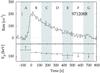 |
Fig. 17 Top panel: 40–700 keV time profile of 971208B. Bottom panel: peak energy evolution. Shaded areas identify the different 128-s intervals over which an average spectrum was acquired. |
4.9.1. Very long GRBs
We examined three of the longest GRBs of our set, which happened to be sampled at several time intervals. For these GRBs we provide a more detailed analysis of how Ep evolves with time compared with the time profile. Figures 17–19 show 971208B, 001213, and 010324, respectively: each top panel shows the 40–700 keV time profile with the typical error bar shown in the upper left corner, while the bottom panel shows the peak energy of the corresponding time intervals as a function of time. These GRBs confirm the variety of Ep evolution compared with the light curves: in the case of 971208B, Ep steadily declined with time even during the rise of the single, long-lasting pulse. In contrast, in the other cases it remains roughly constant throughout different emitting episodes, followed by a final drop at the end of the prompt light curve.
Thanks to its very long duration, the case of 9701208B offers the opportunity to study the relation between the average flux and Ep in each interval. The result is shown in Fig. 20. The best-fitting power law relation is parametrised as by Eq. (8):  (8)The best-fitting parameters computed over the four intervals with measured Ep, from “B” to “E”, are m = 0.32 ± 0.15 and q = 4.36 ± 1.00. Only spectrum “A” taken during the rise in the pulse is not compatible with the pow, and this was already observed in other bursts with a broader energy coverage down to X-rays for a sample of bursts detected with both the Wield Field Cameras (WFC) and the GRBM aboard BeppoSAX (Frontera et al. 2010; Frontera et al., in prep.). This burst is also interesting because it belongs to the FRED (fast rise exponential decay) class, a family of bursts with a single pulse, which are thought to be the building blocks of more complex time profiles (e.g. Norris et al. 1996). Similar results in the Ep evolution of FRED GRBs are discussed by Peng et al. (2009b).
 |
Fig. 20 Peak energy vs. average flux for 971208B. The dashed line is the best-fitting power law with a slope of 0.32 ± 0.15. Labelled spectra are the same as Fig. 17. |
5. Discussion and conclusions
We have analysed the spectral properties of the 185 brightest BeppoSAX/GRBM GRBs, using three different spectral models. The sample includes bright GRBs with a threshold on fluence of Φ > 4.4 × 10⁻⁶ erg cm-2 in the 40–700 keV band; as a consequence, no short duration GRB was selected. The GRBM data used consist of 240-energy channel spectra in the 40–700 keV range continuously integrated over 128 s independently of the onboard trigger logic. For this reason, the analysis mainly concerned the time-integrated spectra of the GRBs; for a number of them, especially the very long ones, it was possible to carry out the spectral analysis for a few contiguous time intervals separately, and these cases are referred to as time-resolved spectra.
About 35% of the sample are best fit with a pow, where the median value of the index is very close to 2. The analogous fraction for the Fermi/GBM, the brightest BATSE, and the Swift known-z GRBs samples is 30%, 21%, and 38%, respectively (Nava et al. 2010). The power law index distribution is centred on αpow = 1.86 ± 0.32 and agrees with other experiments (Sakamoto et al. 2008a; Vianello et al. 2009). GRBs with αpow > 2 (αpow < 2) have a peak energy either close to or below (above) the GRBM lower (upper) bound, so Ep ≲ 40 keV (Ep ≳ 700 keV).
The typical long and bright GRBs are well fit with either a cpl or with a band function. With the GRBM data in none of the cases, the latter model provided a significant improvement with respect to the former. We also proved that, within the accuracy limits of these data, the two models provide consistent estimates for both the low-energy photon index α and the peak energy Ep, although the cpl model tends to overestimate Ep with respect to the band function.
For a sample of 28 GRBs commonly detected by both GRBM and BATSE and for which K06 provided the results of the time-average spectral fitting, we carried out a comparative analysis to establish possible discrepancies and to evaluate the effects of measuring the same quantities with two different instruments. The two sets of α and Ep substantially agree with one another, except for a very few cases that we investigated and for which the main source of discrepancy must be searched in the different time coverage. A strong spectral evolution, observed for several GRBs, can explain why different time intervals may yield significantly different results in the spectral parameters. Specifically to Ep, we modelled all these sources of discrepancy in terms of an additional scatter of about 26% between the GRBM and BATSE Ep estimates. In practice, this has little impact on the known correlations (Amati et al. 2002; Ghirlanda et al. 2004) in which Ep is a key observable.
The observed distribution of Ep peaks around 240 keV with a dispersion of 0.2 dex, very similar to that of bright BATSE bursts (K06; Nava et al. 2010). Its narrowness is explained by the finite passband of the GRBM and of the analogous experiments. That these selection effects connected with data truncation affect the distribution, as discussed in Sect. 4.3, is directly proven by analogous studies carried out over broader energy ranges. Indeed, in the X-ray domain (Frontera et al. 2000; Barraud et al. 2003; Amati 2006; Pelangeon et al. 2008; Sakamoto et al. 2008b) the number of X-ray rich GRBs and XRFs increases remarkably: as a result, the Ep distribution forms a continuum over a correspondingly broad energy band (Sakamoto et al. 2008b). Moreover, the selected sample is not representative of the entire population but only of the brightest end. A number of the GRBs included in our sample and best fit with a soft photon index are likely to have Ep between the XRFs and the hardest GRBs.
The α distribution has its mode around 1 with a dispersion of 0.32 (Fig. 5) so very similar to the dispersion of 0.25 found for both low- and high-energy indices by K06 on a sample of bright BATSE GRBs. In this respect our results agree with catalogue properties of other experiments (Preece et al. 2000; Ghirlanda et al. 2002; K06; Sakamoto et al. 2008a; Nava et al. 2010). For the GRBs with Ep < 100 ÷ 150 keV, α is poorly constrained and is slightly biased towards soft values (Fig. 7). As discussed in Sect. 4.3, this is an instrumental effect that limits the capability of correctly measuring the low-energy photon index when Ep lies close to the lower energy bound. For this sort of GRB, the spectrum cannot reach the asymptotic slope at the lower bound, so the value provided by the fitting procedure turns out to be softer than the asymptotic one (Lloyd & Petrosian 2000; Amati et al. 2002). How close the observed slope can be with respect to its asymptote depends on the spectrum itself and on its physical origin. For instance, assuming the validity of the synchrotron shock model, Lloyd & Petrosian (2000) studied how the smoothness of the cutoff in the electron energy distribution and the distribution of the pitch angle determine how quickly the asymptotic value of α is reached within a given energy passband.
As also noted by K06, the α distribution does not exhibit any clustering around characteristic values expected from various models: 2/3 for synchrotron with no cooling (Katz 1994; Cohen et al. 1997; Tavani 1996), 0 for jitter radiation expected in the case of synchrotron radiation in highly non-uniform short-scale magnetic fields (Medvedev 2000), and 3/2 for fast-cooling synchrotron (Ghisellini et al. 2000).
About 30% of GRBs whose time-average spectrum is best fit with a cpl lie below the synchrotron death line of α = 2/3 (Fig. 5). This fraction is comparable to the one found in BATSE GRB samples (Preece et al. 1998). On the other side of the distribution, the fast-cooling death line represented by the limit α < 3/2 is satisfied by all GRBs. However, the synchrotron process has several problems: the observed distribution around 1 is remarkably harder than the 3/2 expected for a population of cooling electrons in the fast regime. Ghisellini et al. (2000) considered several options for overcoming this discrepancy (particle re-acceleration, deviations from equipartition, quickly varying magnetic fields, adiabatic losses) concluding that the prompt spectrum could not be the result of ultrarelativistic electrons emitting synchrotron and inverse Compton radiation. Alternatively, Lloyd & Petrosian (2000) find that spectra below the synchrotron death line are still possibly produced via synchrotron, provided that one assumes small pitch angles for the emitting electrons. Other possible explanations include synchrotron self-absorption in the X-ray (Granot et al. 2000), the presence of a photospheric component and pair formation (Meszaros & Rees 2000; Ioka et al. 2007), synchrotron self-Compton upscattered to X-rays from optical (Panaitescu & Meszaros 2000), time dependent acceleration and radiation (Lloyd & Petrosian 2002), the decay of magnetic fields (Pe’er & Zhang 2006), the Klein-Nishina effect on synchrotron self-Compton process (Derishev et al. 2001), or continuous electron acceleration as a consequence of plasma turbulence in the post-shock region (Asano & Teresawa 2009).
We have confirmed the correlation between the observed peak energy Ep and the 40–700 keV fluence Φ with a null hypothesis probability of 1.4 × 10⁻⁷. The slope of 0.21 ± 0.06 agrees with previous values obtained on samples of BATSE GRBs: 0.28 ± 0.04 (Lloyd et al. 2000), 0.16 ± 0.02 (Nava et al. 2008). The extrinsic scatter is σlog Ep = 0.13 ± 0.02 (Fig. 10). The observed slope is likely to only be barely affected by data truncation and selection effects. In the literature, the same problem, affecting analogous samples from other experiments like BATSE, was circumvented by means of non-parametric techniques set up to correct for data truncation. Furthermore, this was also done through the analysis of subsamples of brighter GRBs, less affected by selection effects of the detector threshold, as is also the case for our sample. Results on the Ep–Φ correlation based on a proper treatment of these effects provided similar results on the correlation slope (see Lloyd et al. 2000, and references therein).
That the slope is shallower than ~0.5, the slope of the intrinsic Ep,i–Eiso relation (Amati et al. 2002), is explained by a combination of different factors. i) In the observer frame, observables are not redshift-corrected. From the selection effects on Eiso with redshift (both observational and evolutionary), the farthest GRBs have the largest Eiso: this makes the Ep–Φ relation flatter than the intrinsic one. ii) The difficulty of detecting GRBs with Ep values either close to or below the lower bound of the GRBM passband of 40 keV, as suggested by Nava et al. (2008) for BATSE, is an instrumental effect that limits the dynamical range, thus leading to a flatter slope. This seems to be confirmed by the results of Sakamoto et al. (2008b), who find a slope of 0.52 ± 0.11 for an extended sample of BATSE, HETE–II, and Swift GRBs, much more sensitive to lower Ep than the GRBM alone. Although the extrinsic scatter found for the Ep–Φ relation is smaller than that of the intrinsic relation (~0.2), this must be compared with the dynamical range along Ep. Moving from the observer to the intrinsic plane, the ratio between scatter and range along Ep significantly decreases, and the correlation becomes more significant (Amati et al. 2009).
In addition to the α distribution problem suffered by the synchrotron, the dependence of Ep on the prompt emission radius r is strong. Assuming a fixed magnetic field fraction ϵB of the central luminosity L, it is ϵB L ≃ Γ2 B2 r2 c (where Γ is the bulk Lorentz factor of the baryonic outflow and B the magnetic field). If particles are accelerated at the shocks to random Lorentz factor γ, then Ep is expected to be 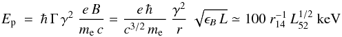 (9)where we adopted the notation Q = Qn × 10n for a generic quantity Q and assumed γ ~ mp/me. Equation (9) naturally explains the Ep,i–L relation, i.e. the time-resolved version of the Ep,i–Eiso relation (Amati et al. 2002). However, relating r to the minimum observed variability timescale, r ~ c tv Γ2, implies the dependence of Ep on Γ, thus making the interpretation of the Ep,i–Liso relation through Eq. (9) troublesome. The resulting dependence of Ep on tv is not observationally established (Lyutikov 2010). Recently, high-energy observations with Fermi of prompt-GeV correlated photons of GRB 080916C (Abdo et al. 2009a) would imply r ~ 1016 cm (based on the constraints derived from the observations of GeV photons and minimum variability timescale in the light curve prompt), while the observed Ep of ~500 keV (Golenetskii et al. 2008) with time-resolved peaks up to a few MeV (Abdo et al. 2009a) is much larger than what is expected from Eq. (9). The same arguments hold for other high-energy GRBs detected with Fermi, such as GRB 090217A (Ackermann et al. 2010) and GRB 090902B (Abdo et al. 2009b).
Overall, the synchrotron shock model cannot account for the entire observed phenomenology of the GRB prompt emission (Kumar et al. 2007; Kumar & McMahon 2008; Kumar & Narayan 2009). As an alternative to the fireball model, in which most of the energy is initially bulk kinetic energy of a relativistic outflow turning into radiation through shocks, electromagnetic models have also been proposed in which the bulk energy is carried by magnetic fields and particle acceleration occurs through magnetic dissipation instead of shocks (Lyutikov 2006, and references therein).
More generally, the magnetic energy content of the ejecta can be explored effectively through early polarisation measurements, when most of the radiation comes from the ejecta themselves rather than the shocked interstellar medium as observed in the afterglow. At optical wavelengths this is thought to be the case whenever a reverse shock, which propagates through the ejecta, dominates the observed radiation during the γ-ray prompt emission or immediately afterwards (e.g., Zhang & Kobayashi 2005). This kind of measurement can distinguish between the different possible origins of the magnetic field: either a large-scale magnetic field originating at the central engine and carried forward by the ejecta or a magnetic field generated in situ through the shocks. Although this kind of measurement is still in its infancy and more data are required to draw firm conclusions, early results on two recent bursts support the large-scale magnetic field scenario within ejecta with comparable magnetic and kinetic energy contents (Mundell et al. 2007; Steele et al. 2009).
Finally, for the longest GRBs it was possible to perform a time-resolved analysis with temporal resolution bound to 128 s. We confirmed the absence of a general evolution of the spectral parameters, especially Ep, throughout the GRB time profile: either a monotonic decline irrespective of the light curve or no remarkable evolution at all. In the case of 971208B, an almost 103-s long FRED, we tracked the spectral evolution in the Ep-flux observer plane, finding it consistent with the Ep,i–L relation (Yonetoku et al. 2004; Ghirlanda et al. 2005), except for the spectrum of the pulse rise, clearly incompatible with it (Fig. 20). This behaviour appears to be naturally explained in the context of synchrotron emission (Eq. (9)), although the issues mentioned above must also be considered. Tracking the peak energy evolution over a broader energy band down to X-rays will be crucial to test the validity limits of this relation better across individual GRBs, as well as samples of GRBs and, consequently, to gain insight into the nature of the dominant emission process during the GRB itself. The importance of a broad band coverage is already shown by the time-resolved combined spectral study with WFC and GRBM aboard BeppoSAX on a sample of GRBs detected with both instruments (Frontera et al. 2010; Frontera et al., in prep.), as well as by the broadband spectral analysis of X-ray flares detected with Swift (Margutti et al. 2010). These capabilities will be key with future missions like SVOM (Dong et al. 2010) and MIRAX (Braga & Mejía 2006; Braga et al. 2010).
Available at http://saxgrbm.iasfbo.inaf.it
Acknowledgments
We thank L. Nava for kindly supplying us with her data. This work is supported by ASI contract ASI-INAF I/088/06/0 “Studio di Astrofisica delle Alte Energie”. We also thank the referee Vahé Petrosian for his useful comments, that led to improvements in the paper.
References
- Abdo, A. A., Ackermann, M., Arimoto, M., et al. 2009a, Science, 323, 1688 [Google Scholar]
- Abdo, A. A., Ackermann, M., Ajello, M., et al. 2009b, ApJ, 706, L138 [NASA ADS] [CrossRef] [Google Scholar]
- Ackermann, M., Ajello, M., Baldini, M., et al. 2010, ApJ, 717, L127 [NASA ADS] [CrossRef] [Google Scholar]
- Amati, L. 2006, MNRAS, 372, 233 [NASA ADS] [CrossRef] [Google Scholar]
- Amati, L., Frontera, F., Tavani, M., et al. 2002, A&A, 390, 81 [NASA ADS] [CrossRef] [EDP Sciences] [Google Scholar]
- Amati, L., Frontera, F., & Guidorzi, C. 2009, A&A, 508, 173 [NASA ADS] [CrossRef] [EDP Sciences] [Google Scholar]
- Arnaud, K. A. 1996, in Astronomical Data Analysis Software and Systems V, ed. G. H. Jacoby, & J. Barnes, ASP Conf. Ser., 101, 17 [Google Scholar]
- Asano, K., & Teresawa, T. 2009, ApJ, 705, 1714 [NASA ADS] [CrossRef] [Google Scholar]
- Band, D., Matteson, J., Ford, L., et al. 1993, ApJ, 413, 281 [NASA ADS] [CrossRef] [Google Scholar]
- Barraud, C., Olive, J.-F., Lestrade, J. P., et al. 2003, A&A, 400, 1021 [NASA ADS] [CrossRef] [EDP Sciences] [Google Scholar]
- Boella, G., Butler, R. C., Perola, G. C., et al. 1997, A&AS, 122, 299 [NASA ADS] [CrossRef] [EDP Sciences] [Google Scholar]
- Braga, J., & Mejía, J. 2006, Proc. SPIE, 6266, 62660M [NASA ADS] [CrossRef] [Google Scholar]
- Braga, J., et al. 2010, IJMPD, Proc. of 2nd Galileo-Xu Guangqi Meeting, held in Villa Hanbury in July, ed. P. Chardonnet, L.-Z. Fang, & R. Ruffini, in press [Google Scholar]
- Cabrera, J. I., Firmani, C., Avila-Reese, V., et al. 2007, MNRAS, 382, 342 [NASA ADS] [CrossRef] [Google Scholar]
- Calura, F., Rapisarda, M., Frontera, F., et al. 2000, Proc. AIP, 526, 721 [CrossRef] [Google Scholar]
- Campana, S., Guidorzi, C., Tagliaferri, et al. 2007, 472, 395 [Google Scholar]
- Cohen, E., Katz, J. I., Piran, T., et al. 1994, ApJ, 488, 330 [Google Scholar]
- Derishev, E. V., Kocharovsky, V. V., & Kocharovsky, Vl.V. 2001, A&A, 372, 1071 [NASA ADS] [CrossRef] [EDP Sciences] [Google Scholar]
- Dong, Y. W., Wu, B. B., Li, Y. G., et al. 2010, Sc. Ch. G., 53, 40 [CrossRef] [Google Scholar]
- Feroci, M., Frontera, F., Costa, E. et al. 1997, Proc. SPIE, 3114, 186 [Google Scholar]
- Frontera, F., Costa, E., Dal Fiume, D., et al. 1997, A&AS, 122, 357 [NASA ADS] [CrossRef] [EDP Sciences] [Google Scholar]
- Frontera, F., Amati, L., Costa, E., et al. 2000, ApJS, 127, 59 [Google Scholar]
- Frontera, F., Guidorzi, C., Montanari, E., et al. 2009, ApJS, 180, 192 (F09) [NASA ADS] [CrossRef] [Google Scholar]
- Frontera, F., Amati, L., Guidorzi, C., Landi, R., & La Parola, V. 2010, Mem. Sos. Astron. Ital., 81, 426 [NASA ADS] [Google Scholar]
- Ghirlanda, G., Celotti, A., & Ghisellini, G. 2002, A&A, 393, 409 [NASA ADS] [CrossRef] [EDP Sciences] [Google Scholar]
- Ghirlanda, G., Ghisellini, G., & Lazzati, D. 2004, ApJ, 616, 331 [NASA ADS] [CrossRef] [Google Scholar]
- Ghirlanda, G., Ghisellini, G., Firmani, C., Celotti, A., & Bosnjak, Z. 2005, MNRAS, 360, L45 [NASA ADS] [CrossRef] [Google Scholar]
- Ghirlanda, G., Nava, L., Ghisellini, G., & Firmani 2007, A&A, 466, 127 [NASA ADS] [CrossRef] [EDP Sciences] [Google Scholar]
- Ghisellini, G., Celotti, A., & Lazzati, D. 2000, MNRAS, 313, L1 [NASA ADS] [CrossRef] [Google Scholar]
- Golenetskii, H., Aptekar, R., Mazets, E., et al. 2008, GCN Circ., 8258 [Google Scholar]
- Granot, J., Piran, T., & Sari, R. 2000, ApJ, 534, L163 [NASA ADS] [CrossRef] [PubMed] [Google Scholar]
- Guidorzi, C. 2002, PhD. Thesis, Univ. of Ferrara [Google Scholar]
- Guidorzi, C., Frontera, F., Montanari, E., et al. 2006, MNRAS, 371, 843 [Google Scholar]
- Heise, J., in’ t Zand, J., Kippen, R. M., & Woods, P. M. 2001, in Gamma-Ray Bursts in the Afterglow Era, ed. E. Costa, F. Frontera, & J. Hjorth (Berlin: Springer), 16 [Google Scholar]
- Ioka, K., Murase, K., Toma, K., et al. 2007, ApJ, 670, L77 [NASA ADS] [CrossRef] [Google Scholar]
- Kargatis, V. E., Liang, E. P., Hurley, K. C., et al. 1994, ApJ, 422, 260 [NASA ADS] [CrossRef] [Google Scholar]
- Kaneko, Y., Preece, R. D., Briggs, M. S., et al. 2006, ApJS, 166, 298 (K06) [NASA ADS] [CrossRef] [Google Scholar]
- Katz, J. I. 1994, ApJ, 432, L107 [NASA ADS] [CrossRef] [Google Scholar]
- Kumar, P., & McMahon, E. 2008, MNRAS, 384, 33 [NASA ADS] [CrossRef] [Google Scholar]
- Kumar, P., & Narayan, R. 2009, MNRAS, 395, 472 [NASA ADS] [CrossRef] [Google Scholar]
- Kumar, P., McMahon, E., Panaitescu, A., et al. 2007, MNRAS, 376, L57 [NASA ADS] [Google Scholar]
- Lloyd, N. M., & Petrosian, V. 1999, ApJ, 511, 550 [NASA ADS] [CrossRef] [Google Scholar]
- Lloyd, N. M., & Petrosian, V. 2000, ApJ, 543, 722 [NASA ADS] [CrossRef] [Google Scholar]
- Lloyd, N. M., Petrosian, V., & Mallozzi, R. S. 2000, ApJ, 534, 227 [NASA ADS] [CrossRef] [Google Scholar]
- Lloyd-Ronning, N. M., & Petrosian, V. 2002, ApJ, 565, 182 [NASA ADS] [CrossRef] [Google Scholar]
- Lyutikov, M. 2006, New J. Phys., 8, 119 [NASA ADS] [CrossRef] [Google Scholar]
- Lyutikov, M. 2010, Conf. Procs The Shocking Universe meeting, Venice, ed. G. Chincarini, P. D’Avanzo, R. Margutti, & R. Salvaterra, SIF, Bologna, 102, 3 [Google Scholar]
- Margutti, R., Guidorzi, C., Chincarini, G., et al. 2010, MNRAS, 406, 2149 [NASA ADS] [CrossRef] [Google Scholar]
- Mc Breen, S., Krühler, T., Rau, A., et al. 2010, A&A, 516, A71 [NASA ADS] [CrossRef] [EDP Sciences] [Google Scholar]
- Medvedev, M. V. 2000, ApJ, 540, 704 [Google Scholar]
- Meegan, C. A., Fishman, G. J., Wilson, R. B., et al. 1992, Nature, 355, 143 [NASA ADS] [CrossRef] [Google Scholar]
- Meszaros, P., & Rees, M. J. 2000, ApJ, 530, 292 [NASA ADS] [CrossRef] [Google Scholar]
- Mundell, C. G., Steele, I. A., Smith, R. J., et al. 2007, Science, 315, 1822 [NASA ADS] [CrossRef] [PubMed] [Google Scholar]
- Nava, L., Ghirlanda, G., Ghisellini, G., & Firmani, C. 2008, MNRAS, 391, 629 [Google Scholar]
- Nava, L., Ghirlanda, G., Ghisellini, G., & Celotti, A. 2010, A&A, submitted [arXiv:1004.1410] [Google Scholar]
- Norris, J. P., Nemiroff, R. J., & Bonnell, J. T. 1996, ApJ, 459, 393 [NASA ADS] [CrossRef] [Google Scholar]
- Paciesas, W. S., Meegan, C. A., Pendleton, G. N., et al. 1999, ApJS, 122, 465 [NASA ADS] [CrossRef] [Google Scholar]
- Panaitescu, A., & Meszaros, P. 2000, ApJ, 544, L17 [NASA ADS] [CrossRef] [Google Scholar]
- Papathanassiou, H. 1999, A&AS, 138, 525 [Google Scholar]
- Pe’er, A., & Zhang, B. 2006, ApJ, 653, 454 [NASA ADS] [CrossRef] [Google Scholar]
- Pelangeon, A., Atteia, J.-L., Nakagawa, Y. E., et al. 2008, A&A, 491, 157 [NASA ADS] [CrossRef] [EDP Sciences] [Google Scholar]
- Peng, Z. Y., Ma, L., Lu, R. J., et al. 2009a, New A, 14, 311 [NASA ADS] [CrossRef] [Google Scholar]
- Peng, Z. Y., Ma, L., Zhao, X. H., et al. 2009b, ApJ, 698, 417 [NASA ADS] [CrossRef] [Google Scholar]
- Preece, R. D., Briggs, M. S., Mallozzi, R. S., et al. 1998, ApJ, 506, L23 [NASA ADS] [CrossRef] [Google Scholar]
- Preece, R. D., Briggs, M. S., Mallozzi, R. S., Pendleton, G. N., & Paciesas, W. S. 2000, ApJS, 126, 19 [NASA ADS] [CrossRef] [Google Scholar]
- Sakamoto, T., Lamb, D. Q., Kawai, N., et al. 2005, ApJ, 629, 311 [NASA ADS] [CrossRef] [Google Scholar]
- Sakamoto, T., Barthelmy, S. D., Barbier, L., et al. 2008a, ApJS, 175, 179 [NASA ADS] [CrossRef] [Google Scholar]
- Sakamoto, T., Hullinger, D., Sato, G., et al. 2008b, ApJ, 679, 570 [NASA ADS] [CrossRef] [Google Scholar]
- Sari, R., Piran, T., & Narayan, R. 1998, ApJ, 497, L17 [NASA ADS] [CrossRef] [Google Scholar]
- Steele, I. A., Mundell, C. G., Smith, R. J., Kobayashi, S., & Guidorzi, C. 2009, Nature, 462, 767 [NASA ADS] [CrossRef] [PubMed] [Google Scholar]
- Tavani, M. 1996, ApJ, 466, 768 [NASA ADS] [CrossRef] [Google Scholar]
- Vianello, G., Götz, D., & Mereghetti, S. 2009, A&A, 495, 1005 [NASA ADS] [CrossRef] [EDP Sciences] [Google Scholar]
- Yonetoku, D., Murakami, T., Nakamura, T., et al. 2004, ApJ, 609, 935 [NASA ADS] [CrossRef] [Google Scholar]
- Zhang, B., & Kobayashi, S. 2005, ApJ, 628, 315 [NASA ADS] [CrossRef] [Google Scholar]
All Tables
Spectral fitting results of the time-integrated spectra for each bright GRB. Frozen values are reported among square brackets.
Spectral fitting results of the time-resolved spectra for each bright GRB that were sampled by more 128-s time intervals.
All Figures
|
Fig. 1 1-s light curve of GRB 000226 detected with GRBM unit 2 in the 40–700 keV band shown as an example. The dashed horizontal line shows the parabolic fit to the background. The vertical lines mark the time intervals corresponding to the 128-s spectra continuously acquired. Spectra “A” and “B” include the GRB, while the adjacent intervals are used to interpolate the background in each channel. |
| In the text | |
|
Fig. 2 128-s light curve of energy channel 60 (160–163 keV) of GRB 000226 as seen with GRBM unit 2 (same example as in Fig. 1). The dashed line shows the linear fit of the background. Same vertical lines as in Fig. 1. |
| In the text | |
|
Fig. 3 Goodness of the fit for all the brightest GRBs with known arrival direction (143 out of 200) as a function of the BeppoSAX local azimuth angle φ. Vertical dashed lines at φ = 0°,90°,180°,270° correspond to the axes of GRBM units 2, 3, 4, 1, respectively. Empty squares (filled circles) are the GRBs localised by other experiments (GRBM alone), as reported in F09. |
| In the text | |
|
Fig. 4 Same as Fig. 3. Angle θ is the BeppoSAX local altitude above the equatorial plane, marked by the vertical dashed line. |
| In the text | |
|
Fig. 5 Top panel: αpow distribution for 55 GRBs with relative uncertainties smaller than 0.3. Mid panel: αcpl distribution for 77 GRBs with relative uncertainties smaller than 0.5. Bottom panel: alternatively to the cpl model, we show the −αband distribution for 31 GRBs for which the band function provides an acceptable fit, although not significantly better than the cpl. The vertical dotted and dashed lines show the cases α = 2/3 (synchrotron death line) and α = 3/2 (cooling death line). In each panel dashed distributions show the corresponding best-fitting Gaussian functions. |
| In the text | |
|
Fig. 6 Peak energy distribution derived with the cpl model for a sample of 106 GRBs with a relative uncertainty smaller than 40%. The dashed line shows the best-fitting normal distribution. |
| In the text | |
|
Fig. 7 Low-energy photon index vs. peak energy as determined with the cpl model on a sample of 70 GRBs with relatively accurate measurements. |
| In the text | |
|
Fig. 8 High-energy photon index β distribution of the band function for a sample of 17 GRBs. |
| In the text | |
|
Fig. 9 Cumulative fluence distribution for the subset of GRBs with a relative error on fluence below 20% (shaded histogram). The dashed histogram is the corresponding fluence distribution published by F09 for the entire GRBM catalogue of GRBs, as derived from 2-channel spectra. The solid line shows the power law distribution with index −3/2 expected if GRBs were homogeneously distributed in an Euclidean space throughout the sampled volume. |
| In the text | |
|
Fig. 10 Correlation between Ep and the 40–700 keV fluence for a sample of 108 bright GRBs with well determined values. The dashed line shows the best-fitting power law, with index 0.21 ± 0.06, while the dotted lines include the 1-σ region, where σ = 0.13 is the extrinsic scatter. Inset: distribution of the normalised scatter. The dashed line shows the standardised normal distribution. |
| In the text | |
|
Fig. 11 Peak energy determined with the cpl vs. the same determined with the band function for a sample of 63 GRBs with both measurements. The dashed and dotted lines show the equality and the best-fitting power law relations, respectively. In particular, according to the latter, the peak energy determined with the cpl tends to be ~20% higher than that of the band. |
| In the text | |
|
Fig. 12 Low-energy photon index determined with the cpl vs. the same determined with the band function for a sample of 21 GRBs with both measurements. The dashed and dotted lines show the equality and the best-fitting linear relations, respectively. |
| In the text | |
|
Fig. 13 BeppoSAX/GRBM versus BATSE: low-energy power law spectra as measured with band and cpl models. The dashed line shows the equality line. |
| In the text | |
|
Fig. 14 BeppoSAX/GRBM versus BATSE: peak energy as measured with band and cpl models. The solid line shows the equality line. The dashed and dotted lines show the best-fitting relation and the 1-σ region. |
| In the text | |
|
Fig. 15 Low-energy photon index as a function of time expressed in units of T90 for a subset of GRBs sampled by multiple spectral intervals. Filled circles, empty squares, and triangles correspond to the spectra A, B, and C, respectively. Each arrow tracks the evolution of a given GRB. |
| In the text | |
 |
Fig. 16 Peak energy as a function of time expressed in units of T90. Same as Fig. 15. |
| In the text | |
|
Fig. 17 Top panel: 40–700 keV time profile of 971208B. Bottom panel: peak energy evolution. Shaded areas identify the different 128-s intervals over which an average spectrum was acquired. |
| In the text | |
 |
Fig. 18 GRB 001213. Same plot as Fig. 17. |
| In the text | |
 |
Fig. 19 GRB 010324. Same plot as Fig. 17. |
| In the text | |
|
Fig. 20 Peak energy vs. average flux for 971208B. The dashed line is the best-fitting power law with a slope of 0.32 ± 0.15. Labelled spectra are the same as Fig. 17. |
| In the text | |
Current usage metrics show cumulative count of Article Views (full-text article views including HTML views, PDF and ePub downloads, according to the available data) and Abstracts Views on Vision4Press platform.
Data correspond to usage on the plateform after 2015. The current usage metrics is available 48-96 hours after online publication and is updated daily on week days.
Initial download of the metrics may take a while.