| Issue |
A&A
Volume 526, February 2011
|
|
|---|---|---|
| Article Number | A74 | |
| Number of page(s) | 20 | |
| Section | Extragalactic astronomy | |
| DOI | https://doi.org/10.1051/0004-6361/201015406 | |
| Published online | 23 December 2010 | |
Wide-field VLBA observations of the Chandra deep field South⋆
1
Astronomisches Institut, Ruhr-Universität Bochum, Universitätsstr.
150, 44801
Bochum, Germany
e-mail: This email address is being protected from spambots. You need JavaScript enabled to view it.
2
National Radio Astronomy Observatory, PO Box 0, Socorro, NM,
87801,
USA
3
Istituto di Radioastronomia – INAF, via Gobetti 101, 40129
Bologna,
Italy
4
Dipartimento di Astronomia, Università degli Studi,
via Ranzani 1, 40127
Bologna,
Italy
5
Max-Planck-Institut für Radioastronomie,
Auf dem Hügel 69, 53121
Bonn,
Germany
6
Curtin University of Technology, GPO BOX U1987, Perth, WA
6845,
Australia
7
Australia Telescope National Facility,
PO Box 76, Epping
NSW
1710,
Australia
Received:
16
July
2010
Accepted:
9
November
2010
Abstract
Context. Wide-field surveys are a commonly-used method for studying thousands of objects simultaneously, to investigate, e.g., the joint evolution of star-forming galaxies and active galactic nuclei. Very long baseline interferometry (VLBI) observations can yield valuable input for such studies because they are able to identify AGN unambiguously in the moderate-to-high-redshift Universe. However, VLBI observations of large swaths of the sky are impractical using standard methods, because the fields of view of VLBI observations are on the order of 10′′ or less, and have therefore so far only played a minor role in galaxy evolution studies.
Aims. We have embarked on a project to carry out Very Long Baseline Array (VLBA) observations of all 96 known radio sources in one of the best-studied areas in the sky, the Chandra deep field South (CDFS). The challenge was to develop methods that could significantly reduce the amount of observing (and post-processing) time, making such a project feasible.
Methods. We developed an extension to the DiFX software correlator that allows one to efficiently correlate up to hundreds of positions within the primary beams of the interferometer antennas. This extension enabled us to target many sources simultaneously, at full resolution and high sensitivity, using only a small amount of observing time. The combination of wide fields-of-view and high sensitivity across the field in this survey is unprecedented.
Results. We observed a single pointing containing the CDFS with the VLBA, in which 96 radio sources were known from previous observations with the Australia Telescope Compact Array (ATCA). From our input sample of 96 sources, 20 were detected with the VLBA, and one more source was tentatively detected. The majority of these objects have flux densities in agreement with arcsec-scale observations, implying that their radio emission comes from very small regions. Two objects are visibly resolved. One VLBI-detected object had been classified earlier as a star-forming galaxy. After comparing the VLBI detections to sources found in sensitive, co-located X-ray observations, we find that X-ray detections are not a good indicator for VLBI detections.
Conclusions. We have successfully demonstrated a new extension to the DiFX software correlator, allowing one to observe hundreds of fields of view simultaneously. In a sensitive observation of the CDFS we detect 21% of the sources and were able to reclassify 7 sources as AGN, which had not been identified as such before. Wide-field VLBI survey science is now coming of age.
Key words: techniques: interferometric / galaxies: active / galaxies: evolution
Appendix B and Full Fig. 3 are only available in electronic form at http://www.aanda.org
© ESO, 2010
1. Introduction
VLBI observations provide the highest resolution in observational astronomy, but at the cost of covering only tiny fields of view. Until recently, only objects with brightness temperatures of the order of 106 K and greater could be observed, and since such objects are distributed sparsely on the sky, the small field of view has not been much of a limitation in the past. However, recent advances in technology provide much larger bandwidths in the observations, enabling the detection of much fainter objects. Their density on the sky is so high that many can be found in the antenna primary beams no matter where one looks.
Unfortunately, the long baselines of VLBI observations traditionally allow only objects within a few arcseconds of the phase centre to be observed, before effects arising from time and frequency averaging wash the signal out. The bottleneck has been correlator capacity and post-processing power. Software correlators and, in particular, DiFX (Deller et al. 2007) are much more flexible than traditional correlators, giving observers the possibility to image objects anywhere in the antenna primary beams. We have developed the necessary software, expertise, and techniques to image all known radio sources within the primary beam of the interferometer elements using a single VLBI observation, the results of which we present in this paper.
There are numerous scientific motivations for carrying out wide-field VLBI surveys. One of the most pressing is to identify active galactic nuclei (AGN). For example, Heisler et al. (1998) obtained VLBI detection rates of 0% for starbursts compared to more than 90% for AGNs in their sample of infrared-selected galaxies. However, as instrumental sensitivities increase, VLBI observations have become more sensitive to detection of radio supernovae in the relatively nearby Universe, such as those in Arp 220 (Smith et al. 1998b), and so a VLBI detection no longer unambiguously implies an AGN. For example, Kewley et al. (2000) observed a sample of 61 luminous infrared galaxies and found compact radio cores in 37% of starburst galaxies and 80% of AGNs. However, the radio luminosity distribution of the Kewley et al. compact cores shows a bimodal distribution. Most higher radio luminosity cores (>2 × 10²¹ W Hz-1) are AGNs, while most lower radio luminosity cores (<2 × 10²¹ W Hz-1) are starbursts. We conclude that VLBI detections of high-luminosity radio cores (≫2 × 10²¹ W Hz-1) are almost certainly AGN, whereas lower-luminosity cores may be caused either by AGN or by supernova activity (also Smith et al. 1998a). For our detection limit of ~0.5 mJy, we can be confident that VLBI detections above z > 0.1 represent AGNs. Below this redshift, a VLBI detection is an ambiguous indicator of AGN activity. Furthermore, the amount of radio emission from an AGN does not correlate well with emission at other wavelengths; in particular there appears to be no correlation between a galaxy’s nuclear radio and its large-scale FIR emission (Corbett et al. 2002).
It is now recognised that AGN play an important role in star formation and galaxy evolution. They are found not only in powerful quasars and radio galaxies, but also in the local universe, with radio luminosities as low as 1020 W Hz-1 (e.g., Filho et al. 2006). AGN feedback can either push back and heat the gas, reducing the formation of stars in the galaxy, or compress the gas clouds, triggering the same process. Particularly at high redshift, both AGN and star formation processes are likely to be important in a large fraction of galaxies (Bower et al. 2006), but we can not yet measure the fraction of the luminosity (bolometric and radio) generated by each process, nor how they are influenced by feedback. Whilst observations at other wavelengths, in particular in the optical and X-ray regime, can identify accretion onto black holes, these data cannot reliably indicate whether or not an AGN also produces radio jets which interact with their surroundings.
Furthermore, VLBI observations of a substantial number of galaxies yield information about specific classes of object. For example, the compact steep-spectrum (CSS) and gigahertz-peaked spectrum (GPS) sources make up a significant fraction (10% to 30%, O’Dea 1998) of radio sources. CSS and GPS sources are very small, yet strong radio sources with either steep spectra (α < −0.5, S ∝ να) or spectra that peak between 500 MHz and 10 GHz. Since only bright members of this class have yet been studied with VLBI observations, a wide-field VLBI survey can yield data in a previously inaccessible flux density regime. Another example is the infrared-faint radio sources (IFRS), a mysterious class of object characterised by strong (up to 20 mJy) 1.4 GHz radio emission but a flux density of less than ~1 μJy in the near-IR at 3.6 μm (Norris et al. 2006). It is now established that they host AGN (Norris et al. 2010, Middelberg et al. 2011 and references therein), but their relation to other classes of object is unclear.
The connection between radio and X-ray emission has recently been investigated by Dunn et al. (2010), using a sample of nearby (D < 100 Mpc) X-ray bright elliptical galaxies. They find that almost all sources are also radio emitters and most display a likely interaction between the X-ray and radio emitting plasmas. On the other hand, they find no correlation between radio and X-ray luminosity. For a study of AGN which are not recognised as such in optical observations (“elusive AGN”), Maiolino et al. (2003) used a VLBI-selected sample of 18 galaxies to maximise the probability of X-ray detections. They find that these objects are heavily obscured (column densities exceeding 1024 cm-2) and that their space density is comparable to, or exceeding that of, optically classified Seyferts. We note however, that both works are difficult to compare to what we present here. Dunn et al. (2010) used VLA observations of nearby elliptical galaxies, and even though the sample by Maiolino et al. (2003) was VLBI-selected, the parent samples were chosen for high IR luminosity and detectability with VLBI. In contrast, our sample is only flux density-limited, and we make no further selection.
Throughout the paper, we adopt a flat ΛCDM cosmology with H0 = 71.0, ΩM = 0.27, Ωvac = 0.73.
2. The target sources
Executing a pilot widefield VLBI observation such as the one described below required the development of new processing techniques, their implementation in software and the purchase of necessary computing infrastructure. A perfect test-bed for these techniques was the Chandra deep field South (CDFS). It has rich complementary coverage at many wavelengths, particularly in the radio regime. However, even with novel processing techniques it was not possible to image the entire area contained within the antennas’ primary beams, nor would this be a promising exercise, since any flux detected in the VLBI observations must have been detected in existing compact-array interferometry data because of their sensitivity to lower-brightness temperature sources1. We therefore used the ATCA observations published by Norris et al. (2006) as an input catalogue, and aimed at imaging all 96 targets from that catalogue in a region centred on the GOODS/CDFS and contained within the VLBA primary beam area. An overview of the observed field is given in Fig. 1, and the details of the target sources are listed in Table 1.
The 96 sources in our sample taken from Norris et al. (2006).
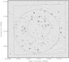 |
Fig. 1 An overview of the observed area. The background image is a radio image of the CDFS made with the Australia Telescope Compact Array (Norris et al. 2006). The rms of the image is around 20 μJy beam-1, and the faintest sources have flux densities of 100 μJy. The square indicates the ECDFS area observed with the Chandra satellite by Lehmer et al. (2005) with an integration time of 240 ks; the large circle indicates a typical VLBA antenna’s primary beam size at the half-power level at 1.4 GHz; and the medium circle is the region covered uniformly with a 2 Ms exposure with Chandra by Luo et al. (2008) (centred on the average aim point with a radius of 7.5′, see their Fig. 2). Crosses are drawn at the locations of the 96 targets taken from Norris et al. (2006) and small circles indicate those targets which were detected with the VLBA. |
3. Observations and data analysis
3.1. Observations
We observed on 3 July 2007 the GOODS/CDFS area with the VLBA at 1383 MHz, centred on RA 03:32:34.0392, Dec −27:50:50.748 (J2000). Two polarisations were recorded across a total bandwidth of 64 MHz, using 2-bit sampling, resulting in a recording bit rate of 512 Mbps. The fringe finders 3C 454.3 and 4C 39.25 were observed in intervals of 2.5 h, and the phase calibrator NVSS J034838−274914 was observed for 1 min after each 5 min scan on the target field. The elapsed time of the observations was 9 h, but the low declination of the target field and the calibrator observations reduced the total integration time on the target field to 178 baseline-hours. According to the VLBA observational status summary2 the baseline sensitivity of the VLBA at 1.4 GHz is 3.3 mJy in a 2 min observation using 256 Mbps recording, or 0.43 mJy per baseline-hour using 512 Mbps. This sensitivity results in a thermal noise limit of our images of 32 μJy beam-1. Accounting for the loss of about 40% of the data in self-calibration on our in-beam calibrator S503 (see Table 1), the estimate has to be increased to about 41 μJy beam-1. However, these estimates are typical of observations near the zenith, but our observations were carried out predominantly at low elevations (at an average elevation of around 20°), where the system temperatures were significantly higher, resulting in a lower expected system sensitivity. For example, the average Tsys of the Fort Davis station when observing the target field was 27% higher than compared to a fringe finder observation at 75° elevation. At Kitt Peak, the increase was 32%, and at Los Alamos 42%. The final on-axis noise was found to be 55 μJy beam-1, only 27% higher than at an average declination of 75°.
3.2. Correlation
3.2.1. Bandwidth and time averaging effects
Since the targets are scattered throughout the primary beam it was necessary to develop new correlation strategies to overcome the effects of bandwidth and time averaging. These effects are commonly called bandwidth smearing and time smearing, since they smear out emission from the target into the map and reduce the observed amplitudes of sources away from the phase centre. Bandwidth smearing is regarded as the aperture synthesis equivalent to chromatic aberration, whereas time smearing can be regarded as similar to motion blur in a photograph when the shutter time is too long. An estimate of the magnitude of these effects can be found in Thompson et al. (2001). In our case, with sources having separations to the phase centre of up to 15 arcmin, and long baselines of typically 5000 km, amplitudes would be reduced to a few percent of their true values if a normal correlator setup with 500 kHz channels and 2 s integrations was used.
To keep the amplitudes within 5% of their true values, one would have to use a channel width of 4 kHz and 50 ms integrations. Such a correlation would result in around 3 TB of visibility data, which would be very difficult to manage even on large general-purpose computers. Furthermore, current hardware correlators are not able to produce data with such high resolution. Therefore the only option was to use a software correlator, in particular the DiFX correlator developed by Deller et al. (2007). We used a development version of DiFX which included a new multiple-field capability, and which was installed on a computer cluster at the Max-Planck-Institut für Radioastronomie in Bonn.
3.2.2. An extension to the DiFX correlator
The DiFX software correlator is widely-used and verified (Deller et al. 2007). It replaced the hardware correlator of the Australian Long Baseline Array in 2008. Subsequent to our observations DiFX has also been adopted as the full-time correlator for the VLBA, and the multiple-field extension capability which is discussed below has recently been incorporated into the VLBA implementation of DiFX and made available to the VLBA community.
The implementation of “simultaneous multiple field centre correlation” is described in detail by Deller et al. (2010), and is briefly summarised here. The correlation is initially performed with high frequency resolution which is sufficient to minimise bandwidth smearing. Periodically, but still frequently enough to minimise time smearing, the phase centre of the correlated data is shifted from its initial location (which is usually the pointing centre) to a target source location. This shift requires rotating the visibility phases of each baseline by an amount equal to the difference in the geometric delay between the final and initial source directions, multiplied by the sky frequency. In effect, this corrects for the “unapplied” differential fringe rotation between the final and initial source directions. This phase shift is repeated for each desired source direction. After the phase shift is applied, the visibilities are averaged in frequency and continue to be averaged in time. Eventually, this results in an array of “normal–sized” visibility datasets, with one dataset per target source. The field of view of each of these datasets is of the order of 13′′, at which point bandwidth and time smearing would reduce the observed amplitudes by 5%.
In comparison to the normal correlation operation, which requires operations on every baseband sample, at a time scale of ~ns, these shift/average operations need only be applied relatively infrequently (10 ms is sufficient to shift past the edge of the primary beam with minimal time smearing), and thus adding many phase centres to the correlation is relatively computationally cheap. Deller et al. (2010) show that hundreds of phase centres can be added within the primary beam at a cost only ~3 times that of a single traditional correlator pass. Hence each individual phase centre requires far fewer operations than a traditional “multi-pass” correlation where the full correlation operation is repeated for each phase centre.
Deller et al. (2010) also demonstrate that the accuracy of the data obtained in this manner is on par with the accuracy of data obtained in the traditional way. Using a small test data set observed at a frequency of 8.4 GHz, they find the amplitude and phase differences of the two methods to be 0.09% and 0.014 ° on average, which is in agreement with effects expected to arise from numerical errors.
3.3. Calibration
3.3.1. Standard steps
The calibration followed standard procedures used in phase-referenced VLBI observations, using the Astronomical Image Processing System, AIPS. Amplitude calibration was carried out using Tsys measurements and known gain curves. Fringe-fitting was carried out on all calibrators to determine delays and phase corrections. The data of the phase calibrator were then exported to Difmap (Shepherd 1997) for imaging. We wrote an extension to Difmap to allow export of the complex gains determined in Difmap to AIPS for further processing3, and to apply the gains to the target data sets. Images were then made of the brighter sources to look for a source suitable for in-beam calibration.
One of the targets, S503, was found to be bright enough for self-calibration. We applied the phase calibrator gains to the S503 data set and used two cycles of phase-only self-calibration to refine the gains, when convergence was reached. Amplitude self-calibration was found to converge on less than 30% of the data and resulted in large gain fluctuations, and was therefore not used on S503. Furthermore, S503 was found to be resolved on long baselines, resulting in the number of useful visibilities reduced by ≈40% after self-calibration. The noise in images (before primary beam correction) was found to be of the order of 55 μJy beam-1. This sensitivity is in reasonable agreement with our expectations, given that (i) the number of visibilities was much reduced in self-calibration, and (ii) the system temperatures in our data were significantly increased compared to observations near the zenith, an effect arising from the average antenna elevations being of the order of only 20 ° (see Sect. 3.1).
Since the phase response of a VLBA antenna is constant within the primary beam, and since the geometric delays had been taken care of at the correlation stage, the amplitude, phase, and delay correction could simply be copied from one target source to another, and an image could be formed. However, another correction is needed to compensate for the amplitude response arising from primary beam attenuation, which reduces the apparent flux density of a source by up to 50%.
3.3.2. Primary beam correction
Unlike in compact-array interferometry, where the primary beam correction is carried
out in the image plane, we corrected for primary beam attenuation by calculating
visibility gains. This is possible only because the fields of view are very small in our
observations and so the attenuation due to the primary beam does not vary significantly
across the image. In general the measured amplitude, A′, of a
visibility is related to the intrinsic amplitude, A, via
 (1)where
g1(t,ν) and
g2(t,ν) are the time and
frequency-dependent gains of the two antennas of the baseline in the direction of the
target. The gains consist of many contributions from various instrumental and
environmental effects, but the attenuation of the signal at each antenna arising from
primary beam attenuation, b1(t,ν) and
b2(t,ν), can be separated, yielding
(1)where
g1(t,ν) and
g2(t,ν) are the time and
frequency-dependent gains of the two antennas of the baseline in the direction of the
target. The gains consist of many contributions from various instrumental and
environmental effects, but the attenuation of the signal at each antenna arising from
primary beam attenuation, b1(t,ν) and
b2(t,ν), can be separated, yielding
 (2)The gains
 and
and
 are determined using
Tsys measurements and antenna gain curves, but the primary
beam attenuation is ignored in standard VLBI calibration procedures because one usually
observes a tiny field of view in direction of the optical axis where these terms can be
ignored.
are determined using
Tsys measurements and antenna gain curves, but the primary
beam attenuation is ignored in standard VLBI calibration procedures because one usually
observes a tiny field of view in direction of the optical axis where these terms can be
ignored.
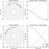 |
Fig. 2 Top left: contour plot illustrating the relative orientation of the LCP (solid lines) and RCP (dashed lines) response of the VLBA antenna at Saint Croix. Contours are drawn at 95%, 90%, 80%, ..., 50% of the peak response. The series of crosses indicates the location of S462 in the antenna’s primary beam during the observations, in intervals of approximately 6 min. Top right: the correction factor required to compensate for primary beam attenuation according to the location of the target, plotted as a function of observing time. The corrections for LCP and RCP can be quite different. Bottom left and right: the same plots for the Mauna Kea station. The series of crosses shows that the correction factors are markedly different from those at Saint Croix, because of the different parallactic angle. |
Two effects need to be taken care of to determine b1(t,ν) and b2(t,ν) at any one time. First, in the case of the VLBA, the receivers are offset from the optical axis, and the beams of the right-hand and left-hand circular polarisations (RCP and LCP) therefore are offset on the sky. This effect is known as beam squint, and it scales with frequency (see Uson & Cotton 2008, for a description of beam squint at the VLA). Second, the beamwidths also are functions of frequency. Since the antennas are alt-azimuth antennas the sources rotate through the two offset beams, and in general sources away from the pointing centre have different parallactic angles, because the separation of the antennas is large (i.e., at any given time antennas see the targets through different portions of their primary beams). This situation is illustrated in Fig. 2. The angular separation (RCP-LCP) between the two beams on the sky, averaged across all 10 antennas of the array, is −1.42′ in azimuth and −0.58′ in elevation (Walker, priv. comm.), or a total of 1.53′, corresponding to 5.4% of the average FWHM. This squint is in good agreement with theoretical predictions (Fomalont & Perley 1999), and is small when the targets are close to the pointing centre (which is half-way between the two beams). However, near the FWHM point of an antenna beam the slope of the beam response is quite steep, and the difference between the RCP and LCP response can be up to 10%.
The beamwidths and the amount and direction of beam squint have been measured at 1438 MHz (Walker, priv. comm.). We scaled these values to the centre frequency of each IF to account for their frequency dependence. The relative locations of the antenna pointing centre, the target coordinates and the RCP and LCP beams on the sky were then computed in 1 min intervals for each IF, and the appropriate correction factor was calculated and saved to a new calibration table. These steps were carried out for each target data set separately.
Primary beam corrections in VLBA observations are uncommon, and this is the first attempt to do so on a larger scale, as far as we are aware. Even though we took care to account for primary beam attenuation as accurately as possible, an amplitude error will unavoidably remain after correction. For example, the quadrupod legs and the subreflector blockage produce errors which have not been accounted for, and the primary beam shape and beam squint are likely to vary with elevation. We estimate that this residual error is of the order of 10%, which we add in quadrature to the other sources of error.
3.3.3. Imaging
We made three images for each source, with increasing resolution. To increase the sensitivity to partially extended sources, we made naturally-weighted images from data with a circular 30% Gaussian taper at a (u,v) distance of 10 Mλ, yielding a resolution of 55.5 × 22.1 mas2. For higher resolution and maximum sensitivity, we made naturally-weighted images using all data, yielding a resolution of 28.6 × 9.3 mas2. For maximum resolution we made uniformly-weighted images using all data, resulting in a resolution of 20.8 × 5.9 mas2. All images were 81922 pixels large, showing areas of 16.4 × 16.4 arcsec2 for the tapered image and 8.2 × 8.2 arcsec2 for the untapered images, respectively. Images were centred on the radio position derived from ATCA observations.
The naturally-weighted and uniformly-weighted images are still plagued by significant imaging artifacts, which we were unable to remove. The sources appear to be irregularly extended predominantly in the north-south direction, in which the resolution is poor because of the low declination of the field. We attribute this to the fact that the visibilities which have the greatest resolution in the north-south direction are preferentially produced near the rise and set of the source. At this time, the airmass is high and these visibilities probably have comparatively large calibration errors. Another effect is that only relatively few long baselines are left after self-calibration on S503, because it is slightly resolved. These visibilities then make a disproportionately large contribution to uniformly-weighted images, reducing their quality. The loss of long baselines in the north-south direction is reflected in a change of the ratio of the restoring beam axes, which increases from 2.51 (tapered images) to 3.1 (natural weighting) and to 3.5 (uniform weighting).
3.4. Source detection and measurements
The target source positions are relatively uncertain, in VLBI terms, as they were determined from arcsec-scale radio observations that have a resolution 500 times lower than the VLBI observations. To account for this, large VLBI images have been made to increase the search space for source emission (see Sect. 3.3.3). We used three criteria to automatically search for potential detections:
-
1.
we computed the SNR of the brightest pixel in the image (excluding a guard band of 100 pixels around the image edges which frequently have artificially high values arising from the imaging procedure). All images with SNR larger than 6 were treated as potential detections;
-
2.
the separation of the brightest pixels in the naturally weighted and tapered images was calculated. If this separation was smaller than a beamwidth, a visual inspection was carried out;
-
3.
we imaged the RCP and LCP data separately, using no taper and natural weighting. Since the two polarisations are processed by different electronics in the antennas, they provide independent information about the sources. These images were set to zero below a threshold, z/
 , with
z = 5σ and σ the noise in the
Stokes I image, and then multiplied. The resulting image is zero everywhere except
at locations where both the RCP and LCP images exceed
z/. Compared to using a simple
5σ cutoff in the Stokes I image this method is less susceptible
to random noise peaks by a factor of more than 6 (see Appendix A).
, with
z = 5σ and σ the noise in the
Stokes I image, and then multiplied. The resulting image is zero everywhere except
at locations where both the RCP and LCP images exceed
z/. Compared to using a simple
5σ cutoff in the Stokes I image this method is less susceptible
to random noise peaks by a factor of more than 6 (see Appendix A).
To measure flux densities of the observed sources requires making a choice about resolution. Many sources are significantly resolved, and almost all sources can be reasonably imaged using heavily tapered or untapered data, resulting in a variety of resolutions. We decided to quote flux densities measured from images tapered at 10 Mλ, because at this resolution all sources (with the exception of S393) can be well approximated by a Gaussian. S393 has been fitted with two Gaussians, and the parameters listed in Table 3 represent their combined values.
Flux densities were measured by fitting a Gaussian to the image, starting at the location of the brightest pixel. The most accurate results were obtained when the shape of the Gaussian was fixed, but its position angle kept as a free parameter. In very low-SNR cases such as ours, free fits frequently result in a gross overestimate of the flux densities.
Flux density errors were estimated as follows. We identified three sources of error: (i) the a priori amplitudes in the VLBI observations are commonly assumed to be to be correct to within 10%; (ii) the formal errors determined by the Gaussian fits; and (iii) the 10% error estimate as a consequence of primary beam correction (which probably is conservative, in particular for sources near the pointing centre). These three components are added in quadrature to yield the total flux density error.
Condon (1997) gives the equations for errors of
Gaussian fits. In our case, the pixels are correlated, in fact, the area over which pixels
are correlated is approximately one resolution element in the images, or one beam area.
For this case, Condon (1997) gives
![Mathematical equation: \begin{equation} \frac{\mu^2(I)}{I^2} \approx \frac{\mu^2(A)}{A^2} + \left(\frac{\theta_{\rm N}^2}{\theta_{\rm M}\theta_{\rm m}}\right)\left[\frac{\mu^2(\theta_{\rm M})}{\theta_{\rm M}^2} + \frac{\mu^2(\theta_{\rm m})}{\theta_{\rm m}^2}\right] \end{equation}](/articles/aa/full_html/2011/02/aa15406-10/aa15406-10-eq55.png) (3)where μ denotes a variance
of a parameter returned by the fitting procedure, I the volume of the
Gauss (the integrated flux density), A its amplitude (the peak flux
density), and θN, θM, and
θm denote the FWHM of a circular Gaussian
convolving function and the major and minor axes of the fit, respectively. In our case,
(3)where μ denotes a variance
of a parameter returned by the fitting procedure, I the volume of the
Gauss (the integrated flux density), A its amplitude (the peak flux
density), and θN, θM, and
θm denote the FWHM of a circular Gaussian
convolving function and the major and minor axes of the fit, respectively. In our case,
 , hence the equation simplifies to
![Mathematical equation: \begin{equation} \frac{\mu^2(I)}{I^2} \approx \frac{\mu^2(A)}{A^2} + \left[\frac{\mu^2(\theta_{\rm M})}{\theta_{\rm M}^2} + \frac{\mu^2(\theta_{\rm m})}{\theta_{\rm m}^2}\right] \end{equation}](/articles/aa/full_html/2011/02/aa15406-10/aa15406-10-eq61.png) (4)which we use as an estimate of the integrated
flux density error arising from the fitting procedure.
(4)which we use as an estimate of the integrated
flux density error arising from the fitting procedure.
4. Results
A summary of the image properties, source flux densities, and ancilliary data is listed in Table 3.
4.1. Images
Contour plots of the 20 detected sources and the one candidate detection are shown in
Fig. 3. The three images per source, made with
different weighting and tapering, are shown in a row. The left panel shows a
naturally-weighted image made with a 10 Mλ tapering (restoring beam size
55.5 × 22.1 mas2), the centre panel the untapered, naturally-weighted image
(restoring beam size 28.6 × 9.3 mas2), and the right panel shows the
uniformly-weighted image (restoring beam 20.8 × 5.9 mas2). Positive contours
start at three times the rms level of the images and increase by factors of
. One negative contour is shown at three
times the rms.
5. Discussion
5.1. Statistics
5.1.1. Detections
One of the goals of this project was to identify AGN in a blind survey of radio sources, i.e., without selecting objects other than by requiring a radio flux density in the ATCA survey. Given that the sensitivity of the VLBI observations varies by a factor of more than two over the observed area, the detection statistics are difficult to analyse. Also, our observations are biased towards compact objects, and this bias is a function of flux density. Fainter sources will only be detected in VLBI observations if they are increasingly compact, whereas strong sources such as S393 (the second-brightest in our sample) can be detected if a fraction as low as 10% is contained within a compact core. This means that the source types that our observations are sensitive to is a function of flux density.
To provide some analysis of the detection statistics despite these shortcomings, we divided our sample into three groups: sources with ATCA flux densities, S, of 10 mJy or more (bin 1, 7 objects), sources with 1 mJy ≤ S < 10 mJy (bin 2, 16 objects), and sources with S < 1 mJy (bin 3, 73 objects).
Out of the three bins, 5, 11 and 5 objects have been detected, respectively, corresponding to percentages of 71%, 69%, and 7% (see Table 2). Most of the VLBA-detected sources (14 sources) are compact, which is indicated by the ratio of VLBI-scale flux density to the ATCA-scale flux density being consistent with unity (see Table 3). We note, however, that the ATCA flux densities by Norris et al. (2006) are probably affected by clean bias, which tends to underestimate the flux densities of weak sources. For a very similar observation, Middelberg et al. (2008a) show that clean bias can decrease the flux density by up to 5% for sources with SNR smaller than 20. Hence the ratio of the VLBI-scale flux density to ATCA-scale flux density is biased towards higher values, in particular for sources with an ATCA flux density of less than 1 mJy, and even exceeds unity in some cases.
The number of observed and detected radio sources.
Results of our observations.
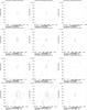 |
Fig. 3 Contour plots of the detected sources. Three images per source are shown in a
row. Left column: naturally-weighted images made with a
10 Mλ tapering (restoring beam size
55.5 × 22.1 mas2); middle column: untapered,
naturally-weighted image (restoring beam size 28.6 × 9.3 mas2);
right column: uniformly-weighted image (restoring beam
20.8 × 5.9 mas2). Positive contours start at three times the rms
level of the images and increase by factors of
|
5.1.2. New AGN
It was noted in the introduction that a detection in a VLBI observation is a strong indicator for AGN activity. To determine whether a source is already a known AGN we used the information from various sources listed in Norris et al. (2006) and the criteria by Szokoly et al. (2004) (using the X-ray hardness ratio and X-ray luminosity, see Sect. 5.2.3).
Without the VLBI data presented here, the combined radio, IR, optical, and X-ray data were able to classify 36 sources (38%) as AGN. There are 7 sources however, which have not been identified as AGN and are detected in the VLBI observations. This number is 7% of the total number of radio objects observed, but 35% of the sources detected with the VLBA.
All VLBI-detected bright sources in bin 1 were known to be AGN before, but out of the 16 medium-bright sources in bin 2, only 10 (63%) were previously known to be AGN, and our VLBA observations have added 5 (31%). Among the 73 faint sources in bin 3, 19 sources were known AGN (26%), and we added 2 (4%). These statistics suggest that VLBI observations can make a significant contribution to the classification of galaxies below a flux density of 10 mJy, because brighter objects are already known AGN, and objects fainter than 1 mJy are only occasionally detected. This ability, of course, is a function of the sensitivity of the VLBI observations, which will soon improve significantly as the bandwidths of radio telescopes increase.
Two sources, S423 and S443, have not been classified as AGN based on their optical and X-ray properties, but are detected in our VLBI observations. In these two cases the ancilliary data indicated a starburst or elliptical and a spiral galaxy, respectively. S423 is detected marginally in the uniformly-weighted image, with a resolution of 20.8 × 5.9 mas2. Its peak flux density is 300 μJy/beam, which indicates a brightness temperatures of 2.2 × 10⁶ K. Hence it displays characteristics of a normal galaxy while at the same time exhibiting a brightness temperature clearly indicating an AGN. The VLBI detection of S443 is offset from the centre of the galaxy and can therefore not be taken as evidence for an AGN; for further discussion on possible origins, see Appendix B. It has also been ignored in the following analyses which compare properties of VLBI-detected and VLBI-undetected sources.
5.1.3. Radio spectral index
Radio spectral index can be used as an indicator for AGN activity. When the spectral index is larger than −0.3 (S ∝ να) then the emission is deemed to come from self-absorbed synchrotron emission such as that found in the very compact regions of AGN and their jets. When the spectral index is smaller than −1.2 then the emission is thought to come from extended structures formed by AGN in the high-redshift Universe. Between these values, a separation between AGN and star-forming activity can not be made. We took the data measured by Kellermann et al. (2008) and found that the median spectral index among the VLBI-detected sources is −0.7, whereas the undetected sources have a median of −0.8. In both cases, the scatter of the distribution as characterised by the median average difference (MAD) is 0.2. A Kolmogorov-Smirnov test (K-S-test) returns a p of 0.80 that the two samples are drawn from the same parent population, indicating that there is no significant difference in spectral index between sources detected and undetected with VLBI.
One might expect that the VLBI-detected sources show higher spectral indices than the undetected sources, because the VLBI observations require the emission to come from smaller regions, which then have a tendency to have smaller optical depths. We argue that since the linear resolution of our observations is of the order of 280 pc (VLBI flux densities were measured from images with a resolution of 55 × 22 mas and a typical redshift is 1) the emission from the observed regions is still dominated by optically thin synchrotron radiation. Unfortunately, the number of VLBI-detected objects is too small to test this hypothesis statistically.
5.1.4. Redshifts
We searched the literature for redshift measurements of our sample. In total, we found redshifts for 82 sources, of which 19 were detected in our VLBA observations. The median redshift of the detected sources is 0.98 with a MAD of 0.29, whereas the undetected sources have a median redshift of 0.67 with a MAD of 0.41. Again the samples are not significantly different, with a p of 0.18 in a K-S-test.
5.1.5. Infrared-Faint Radio Sources (IFRS)
IFRS are mysterious objects which can be strong (tens of mJy) radio sources but do not have near-infrared counterparts detected by the Spitzer observatory as part of the Spitzer Wide-area InfraRed Extragalactic Survey (SWIRE). IFRS are unexpected because all known classes of galaxy at z < 2 are expected to be detectable given the IR survey sensitivities. See Huynh et al. (2010), Norris et al. (2010) and Middelberg et al. (2011) and their references for recent work on these sources. Previous VLBI observations of six IFRS have resulted in two detections (Norris et al. 2007; Middelberg et al. 2008b), supporting the idea that IFRS are AGN-driven. There are three radio sources in our sample which have been classified as IFRS: S415, S446, and S506, which have catalogued arcsec-scale flux densities of 1.2 mJy, 0.3 mJy, and 0.2 mJy, but none was detected.
5.2. Co-located X-ray observations
X-ray observations are claimed to be a very direct tracer of AGN activity (e.g., Mushotzky 2004). The radiation originates very close to the supermassive black hole, it can leave these regions rather unabsorbed, in particular at energies of a few keV, and there is little contamination from other sources, such as stars.
The surveyed region has been observed intensively with the Chandra X-ray observatory. In particular, a 940 ks exposure of a 0.11 deg2 region as indicated in Fig. 1, known as “the” CDFS, has resulted in the detection of 346 sources (Giacconi et al. 2002). The region has been reobserved by Luo et al. (2008), adding more than 1 Ms to the total exposure time and resulting in a central sensitivity of 7.1 × 10⁻¹⁷ erg cm-2 s-1. The total number of X-ray sources found in this observation was 578. Furthermore, a 240 ks exposure of a 0.3 deg2 region, known as the extended Chandra deep field South (ECDFS), covers entirely the area observed here (Lehmer et al. 2005). This observation, with a maximum sensitivity of 3.5 × 10⁻¹⁶ erg cm-2 s-1, yielded the detection of 762 point sources. All observations were carried out in the energy range 0.5–8 keV and provide information about source flux densities in a soft band (0.5–2 keV) and in a hard band (2–8 keV). We cross-matched our detections to these catalogues.
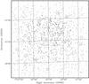 |
Fig. 4 Diagram illustrating the locations of X-ray sources in the CDFS (crosses), in the ECDFS (squares) and the sources detected in our VLBI observations (circles). |
5.2.1. Identifications in the CDFS
The region indicated with the medium circle in Figure 1 contains 23 radio sources, of which 6 were detected by our VLBI observations. A search for counterparts of the VLBI-detected sources in the catalogues by Luo et al. (2008) returned 5 matches. There is only one VLBI-detected source, S474, which clearly lies in the area covered by the X-ray observations, but is not detected in the X-ray. Whilst it lies towards the edge of the area covered by the 2 Ms exposure, the integration times of the sources surrounding S474 suggest that its location has been observed for around 1.3 Ms. A further 4 VLBI-detected sources have X-ray counterparts outside the most sensitive region (see Fig. 4).
5.2.2. Identifications in the ECDFS
Repeating the search in the catalogue by Lehmer et al. (2005), which covers an area that includes all sources observed by us, returned 12 sources, 8 of which were identical to sources discovered in the search of the CDFS data. Hence only one VLBI source was detected in the deep CDFS observations but not in the shallower ECDFS observations. In total 7 VLBI sources have no X-ray counterpart at all.
This result sheds an interesting light on X-ray observations as a means of filtering AGN: at a sensitivity level corresponding to integration times of between 240 ks and 2 Ms the fraction of VLBI-detected AGN with X-ray counterparts increases from 12/20 = 60% to 5/6 = 83%.
5.2.3. Hardness ratios
The hardness ratio 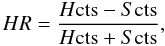 (5)where Hcts and
Scts are the net counts in the hard and soft band, can be used as an
indicator for the degree of obscuration of an object. Soft X-ray spectra (with
HR < −0.2) generally indicate that objects are unobscured and
that, in the case of AGN, one is looking at a type 1 object. Harder spectra
(HR > −0.2) indicate obscured lines of sight as would be caused by
a dusty circumnuclear torus and can therefore be taken as indicators for type 2 objects.
The classification based on hardness ratio alone can be improved when the total X-ray
luminosity is also taken into account, as has been demonstrated by Szokoly et al. (2004). Sources with X-ray luminosities below
1035 W (1042 erg s-1) are treated as non-AGN,
sources with luminosities between 1035 W and 1037 W are considered
as AGN and sources with X-ray luminosities in excess of 1037 W are classified
as QSO. The hardness ratio is then used to further distinguish between type 1 and type 2
objects.
(5)where Hcts and
Scts are the net counts in the hard and soft band, can be used as an
indicator for the degree of obscuration of an object. Soft X-ray spectra (with
HR < −0.2) generally indicate that objects are unobscured and
that, in the case of AGN, one is looking at a type 1 object. Harder spectra
(HR > −0.2) indicate obscured lines of sight as would be caused by
a dusty circumnuclear torus and can therefore be taken as indicators for type 2 objects.
The classification based on hardness ratio alone can be improved when the total X-ray
luminosity is also taken into account, as has been demonstrated by Szokoly et al. (2004). Sources with X-ray luminosities below
1035 W (1042 erg s-1) are treated as non-AGN,
sources with luminosities between 1035 W and 1037 W are considered
as AGN and sources with X-ray luminosities in excess of 1037 W are classified
as QSO. The hardness ratio is then used to further distinguish between type 1 and type 2
objects.
We calculated the hardness ratio for all 13 VLBI-detected sources with X-ray counterparts. Where both Luo et al. (2008) and Lehmer et al. (2005) had made a detection we adopted the measurements of the former observation since it is more sensitive and its errors are smaller. Also note that in the case of sources with very few counts a rigorous error estimate essentially requires a re-analysis of the raw data (Park et al. 2006), which is beyond the scope of this paper. We therefore do not give an error for the hardness ratios. For all 14 objects redshifts were available in the literature, hence the total X-ray luminosity could be calculated and the Szokoly et al. (2004) criteria were used for classification. The scheme resulted in 3 non-AGNs (23%), 2 and 3 type 1/2 AGNs (15% and 23%), respectively, and 5 type 1 QSOs (39%, no type 2 QSOs). Out of the VLBI-undetected sources, 25 had sufficient data available for this classification, resulting in 10 non-AGN (40%), 4 and 11 type 1/2 AGNs (16% and 44%), and no QSOs. See Fig. 5 for an illustration of these statistics. It is difficult to read a trend off this distribution, however, the lack of undetected type 1 QSOs is striking. Whilst only ~10% of optically selected type 1 QSOs are radio-loud, a much larger fraction of X-ray selected type 1 QSOs appear to be radio-loud.
Part of the cause of this effect is that all 5 type 1 QSOs are brighter than 1 mJy, where the fraction of VLBI detections is generally high (69%).
5.2.4. Potential causes of the X-ray non-detections
Since X-ray observations have been claimed to be a very good tracer of AGN activity (e.g., Mushotzky 2004; Brandt & Hasinger 2005), the lack of X-ray counterparts to almost 1/3 of the VLBI-detected sources deserves a closer look.
First, it must be noted that the VLBI-detected source without X-ray counterpart in general have lower flux densities in other bands, too: only one of these objects, S329, does have a measured optical magnitude, and only one other, S519, has a measured 24 μm flux density. One object, S545, does have no optical or infrared flux density at all.
Second, there appears to be no correlation between X-ray and radio flux densities (Fig. 6). Hence some objects will unavoidably have no X-ray counterpart, just as some sources with X-ray detections have no VLBI detection.
Third, some sources could be Compton-thick and be so obscured that they remained undetected in the X-ray observations. This happens at column densities of NH ≫ 1.5 × 1024 cm-2 (Brandt & Hasinger 2005), which reduces the X-ray flux by two orders of magnitude, even at high (>10 keV) energies.
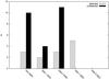 |
Fig. 5 X-ray classification statistics. Cross-hatched bars represent sources with a VLBI detection and black bars sources without. The lack of undetected type 1 QSOs is striking (see discussion in text). |
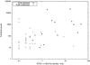 |
Fig. 6 Full-band X-ray counts as a function of 1.4 GHz flux density. Neither the VLBI-detected (asterisks) nor the VLBI-undetected radio sources (pluses) show a correlation with X-ray counts. |
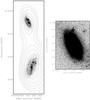 |
Fig. 7 Left panel: HST B-band image of S443 (at the
top) and S442 (bottom). Black contours (starting at
0.1 mJy and increasing by factors of |
6. Conclusions
Wide-field VLBI observations of 96 sources in the CDFS have been carried out using a new correlation technique on a software correlator. The correlation was carried out only once, with high temporal and spectral resolution to avoid averaging effects, and the visibilities were phase-rotated to the 96 target fields inside the correlator, and then averaged. This approach is equivalent to a multi-pass correlation, but requires only a small computational overhead. It results in many small, normal-sized data sets, which can be calibrated using standard techniques. The results of this project are as follows.
-
We have imaged all sources and detected a fraction of 21%. The detection of one additional source is in the outer regions of the optical host galaxy, and could be a radio supernova. Most sources have flux densities of the same order as the arcsec-scale flux densities, and the radio-emitting regions therefore must be smaller than hundreds of pc (or less in some cases). Given their redshifts we can confidently interpret nearly all our VLBI detections as AGN.
-
A search of co-located, sensitive X-ray observations revealed that VLBI observations can identify AGN which have previously been missed, even though X-ray observations are expected to be a very good tracer of AGN activity. A total of 7 sources were classified as AGN for the first time. Using X-ray data alone, only 10 out of the 13 detected sources with available X-ray counterparts were identified as AGN, missing about one-quarter.
-
The VLBI core in the star-forming galaxy S443, which is one of the lowest redshift galaxies in our sample, has a radio luminosity of 5 × 10²¹ W Hz-1, consistent with that of a supernova. The VLBI core in the galaxy S423 at a redshift of 0.73 is surprising, because multiband photometry and X-ray data do not indicate the presence of an AGN.
-
Surprisingly, the VLBI detections include every X-ray detected type 1 QSO in our field, whereas only about 10% of optically-selected type 1 QSOs are radio-loud. Therefore, either X-ray observations preferentially select radio-loud QSOs, or even radio-quiet QSOs have compact cores detectable with VLBI.
Online material
Appendix B: Notes on individual sources
-
S329: this source appears to be mildly resolved in our VLBIimage, and is undetected at 0.5–8 keV byLehmer et al. (2005). Its redshift is1.00 (Mainieri et al. 2008).
-
S331: this source has been classified as AGN because of its more than tenfold radio excess over the radio-infrared relation. Its value of q24 is −1.96 which clearly puts it into the AGN regime. Its X-ray properties (Lehmer et al. 2005; Szokoly et al. 2004) suggest that it is a type 1 AGN.
-
S380: this compact radio object was classified as AGN based on its q24 value of −0.21 (Norris et al. 2006). Its X-ray properties qualify it as a galaxy because its X-ray luminosity in the 0.5–8 keV band is only LX = 4.6 × 1031 W (Lehmer et al. 2005; Szokoly et al. 2004). It has a spectral index of −0.6 (Kellermann et al. 2008) and a redshift of 0.02 (Wolf et al. 2004), making it the closest object in our sample.
-
S393: this is the only VLBI-detected source with a pronounced extension in the VLBI observations. It is an X-ray source at a redshift of 1.07 (Zheng et al. 2004), and it has been identified as AGN by Norris et al. (2006) because of its X-ray hardness ratio. The Szokoly et al. (2004) criteria result in a type 2 AGN classification, and its radio spectral index is −1.2 (Kellermann et al. 2008). Only a very small fraction (5%) of its arcsec-scale flux density is recovered in the VLBI observations. At its redshift, the angular separation of 32 mas of the two components seen in our VLBI images translate to a projected distance of 263 pc, and is therefore in the regime of GPS sources (and is of a size comparable to the narrow-line region).
-
S404: the VLBI images of this source display almost all the flux density found in the ATCA observations. It has a compact morphology and its X-ray properties classify it as a type 1 QSO (Luo et al. 2008; Szokoly et al. 2004). It has a spectral index of 0.0 (Kellermann et al. 2008), indicating a compact, self-absorbed radio source, and its redshift is 0.54 (Norris et al. 2006). The HST images show an unresolved object with diffraction spikes, indicative of a point-like optical source. Its q24, however, is 0.31 which is only a mild radio excess over the radio-infrared relation.
-
S411: this is a compact source – all arcsec-scale emission is recovered in the VLBI image. Its hardness ratio of −0.44 and X-ray luminosity qualify it as a type 1 QSO (Luo et al. 2008; Szokoly et al. 2004) and it is located at a redshift of 1.61 (Afonso et al. 2006). It has a spectral index of −0.5 (Kellermann et al. 2008), and it is a featureless, round object in the HST ACS images (Giavalisco et al. 2004).
-
S414: this is a compact source – the VLBI observations recover 95% of the flux density measured with the ATCA (Norris et al. 2006). It has q24 = −0.29 which makes this an AGN. S414 has a redshift of 1.57 (Mainieri et al. 2008) and is the brightest X-ray source in our sample, with LX = 1.5 × 1038 W (0.5–8 keV), qualifying it as a type 1 QSO (Lehmer et al. 2005; Szokoly et al. 2004).
-
S421: the radio data for this source are consistent with a point source since it is unresolved in our VLBI image. It is not an X-ray source, and it has a spectral index of −0.6 (Kellermann et al. 2008) and a redshift of 0.13 (Mainieri et al. 2008).
-
S423: this compact radio source is classified as a normal galaxy using the scheme by Szokoly et al. (2004). It has a spectral index of −0.2 (Kellermann et al. 2008) and a redshift of 0.73 (Afonso et al. 2006). Afonso et al. report spectroscopic evidence for star-forming activity in this galaxy, potentially merging with a nearby (0.5′′) object. They identify five objects closer than 30′′ with similar redshifts. Mobasher et al. (2004) classify this object as an elliptical galaxy, using photometry in 17 bands. Hence there is no evidence except the VLBI detection that this object harbours an AGN. Given its redshift it has a 5 GHz radio luminosity of 7.5 × 10²³ W Hz-1, which is about an order of magnitude too low to classify it as a radio-loud object, and is more typical of Seyferts.
-
S437: this source has been classified as AGN based on q24 and the literature (Norris et al. 2006). Only 4% of its ATCA flux density were recovered, and the VLBI images show an unresolved source. Yet it is a powerful X-ray source exceeding a luminosity of 1037 W (0.5–8 keV) and it has a hardness ratio of −0.48, indicating a type 1 QSO (Luo et al. 2008; Szokoly et al. 2004). The redshift of this object is 0.73 (Afonso et al. 2006). It is one of four objects covered by the Great Observatories Origins Deep Survey (GOODS, Giavalisco et al. 2004) with the Hubble Space Telescope. It is an unresolved object in all four bands, and diffraction spikes indicate a strong point-like component.
-
S443: this compact object is the faintest VLBI-detected radio source in our survey, with an arcsec-scale flux density of only 0.4 mJy (Norris et al. 2006). It is associated with a spiral galaxy, with a spectral index of −0.5 (Kellermann et al. 2008) and a redshift of 0.076 (Afonso et al. 2006). Its q24 value of 1.05 is broadly consistent with the value of 0.84 found by Appleton et al. (2004) for the radio-infrared relation, and also its X-ray properties suggest that it is a galaxy without AGN. Afonso et al. (2006) report that the X-ray emission comes from north of the galaxy nucleus, with indications of star-forming activity. Mobasher et al. (2004) classify it as an Sbc object based on 18-band photometry. We consider this a marginal detection, partly because the VLBI position places the VLBI source at the very edge of the visible perimeter of the galaxy, which can be treated as evidence against a detection (see Fig. 7). On the other hand, a radio transient cannot be ruled out (see Lenc et al. 2008). We also note that the radio luminosity of this source, 5 × 10²¹ W Hz-1, is similar to one of the brightest radio SNe, SN1986J. We therefore consider it possible that S443 is a radio supernova.
-
S447: this source has been classified as AGN based on q24 and also is an X-ray source. It has a spectroscopic redshift of 1.96 (Norris et al. 2006), where 1 mas corresponds to 8.5 pc. It is unresolved in our images, hence most of the VLBI flux density (20% of the arcsec-scale flux density) comes from a region smaller than ~100 pc. It is the second most luminous X-ray source in our sample of 96 sources, with LX = 1.3 × 1038 W (0.5–8 keV, Lehmer et al. 2005). Nevertheless it has a soft spectrum with HR = −0.37 which qualifies it as a type 1 QSO (Szokoly et al. 2004).
-
S472: this is a very compact source since 93% of the ATCA flux density are seen in the VLBI image. Based on its q24 = −0.31 this is an AGN. There is conflicting information about its redshift: Zheng et al. (2004) give a photometric redshift of 1.22, but Le Fèvre et al. (2004) measured a spectroscopic redshift of 0.55, which we deem more reliable. Its X-ray spectrum is hard between 0.5–8 keV and indicates an absorbed type 2 AGN (Lehmer et al. 2005; Szokoly et al. 2004).
-
S474: this is a compact source which displays all of its ATCA flux density in a low-resolution VLBI image. Its redshift is 0.98 (Le Fèvre et al. 2004) and its spectral index is −1.4 (Kellermann et al. 2008). It is a faint infrared source and is undetected in the X-ray. This is the only VLBI-detected radio source which remained undetected by the 2 Ms Chandra exposure (Luo et al. 2008).
-
S482: this is a compact radio source. It is also an X-ray source (Lehmer et al. 2005) with hardness ratio −0.33, but its luminosity is only LX = 5.2 × 1033 W (0.5–8 keV), which then qualifies it as a galaxy (Szokoly et al. 2004). It was classified by Norris et al. (2006) as an AGN based on its q24 of −0.61. It has a spectral index of −0.5 (Kellermann et al. 2008) and redshift of 0.15 (Norris et al. 2006).
-
S500: this compact radio object has an absorbed X-ray spectrum with hardness ratio 0.6 (Lehmer et al. 2005) , and it is classified as a type 2 AGN by the Szokoly et al. (2004) criteria. It has a spectral index of −0.9 (Kellermann et al. 2008) and a redshift of 0.73 (Mainieri et al. 2008). Based on q24 = −0.21, this is an AGN.
-
S503: this is the brightest source in our VLBI observations, with a flux density of (21.2 ± 3.0) mJy (compared to an ATCA flux density of 19.3 mJy). Hence this source is very compact, but our uniformly-weighted image indicates that its core is resolved into two components with a separation of around 10 mas (76 pc at the distance of S503; z = 0.81, Mainieri et al. 2008). It is an X-ray source indicating a type 1 AGN (Lehmer et al. 2005; Szokoly et al. 2004).
-
S517: this compact radio source is not a detected X-ray source, and it has a spectral index of −0.9 (Kellermann et al. 2008) and a redshift of 1.03 (Mainieri et al. 2008). The extensions towards the south-east seen in the VLBI images are imaging artifacts and do not indicate a true extension.
-
S519: this compact radio source has previously been classified as AGN based on its q24 = −0.42. It is not an X-ray source, and it has a redshift of 0.69 (Norris et al. 2006).
-
S520: this source is mildly resolved. From its arcsec-scale flux density of 3.7 mJy (2.5 ± 0.4) mJy could be recovered in our lowest-resolution image. There is a hint of a ~25 mas extension towards the south-west in the naturally and uniformly-weighted image which at the redshift of the source of 1.4 (Wolf et al. 2004) corresponds to around 200 pc. It has only a very faint IR counterpart in the co-located Spitzer image, and is not detected in the ECDFS survey by Lehmer et al. (2005) (it is outside the GOODS region).
-
S545: this compact radio source also does not exhibit X-ray emission, and neither a spectral nor a redshift are available.
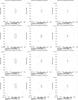 |
Fig. 3 continued. |
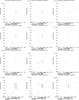 |
Fig. 3 continued. |
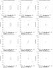 |
Fig. 3 continued. |
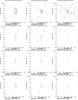 |
Fig. 3 continued. |
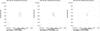 |
Fig. 3 continued. |
This reasoning ignores variability and transient events, see Lenc et al. (2008) for an example.
Acknowledgments
We thank Craig Walker for providing detailed beam width and squint measurements, and for discussions on a primary beam attenuation scheme. We also thank the anonymous referee who has helped to improve this paper considerably. This research has made use of the NASA/IPAC Extragalactic Database (NED) which is operated by the Jet Propulsion Laboratory, California Institute of Technology, under contract with the National Aeronautics and Space Administration.
References
- Afonso, J., Mobasher, B., Koekemoer, A., Norris, R. P., & Cram, L. 2006, AJ, 131, 1216 [Google Scholar]
- Appleton, P. N., Fadda, D. T., Marleau, F. R., et al. 2004, ApJS, 154, 147 [NASA ADS] [CrossRef] [Google Scholar]
- Bower, R. G., Benson, A. J., Malbon, R., et al. 2006, MNRAS, 370, 645 [NASA ADS] [CrossRef] [Google Scholar]
- Brandt, W. N., & Hasinger, G. 2005, ARA&A, 43, 827 [Google Scholar]
- Condon, J. J. 1997, PASP, 109, 166 [NASA ADS] [CrossRef] [Google Scholar]
- Corbett, E. A., Norris, R. P., Heisler, C. A., et al. 2002, ApJ, 564, 650 [NASA ADS] [CrossRef] [Google Scholar]
- Deller, A. T., Tingay, S. J., Bailes, M., & West, C. 2007, PASP, 119, 318 [NASA ADS] [CrossRef] [Google Scholar]
- Deller, A. T., Brisken, W. F., Phillips, C. J., et al. 2010, ApJ, submitted [Google Scholar]
- Dunn, R. J. H., Allen, S. W., Taylor, G. B., et al. 2010, MNRAS, 404, 180 [NASA ADS] [Google Scholar]
- Filho, M. E., Barthel, P. D., & Ho, L. C. 2006, A&A, 451, 71 [NASA ADS] [CrossRef] [EDP Sciences] [Google Scholar]
- Fomalont, E. B., & Perley, R. A. 1999, in Synthesis Imaging in Radio Astronomy II, ed. G. B. Taylor, C. L. Carilli, & R. A. Perley, ASP Conf. Ser., 180, 79 [Google Scholar]
- Giacconi, R., Zirm, A., Wang, J., et al. 2002, ApJS, 139, 369 [NASA ADS] [CrossRef] [Google Scholar]
- Giavalisco, M., Ferguson, H. C., Koekemoer, A. M., et al. 2004, ApJ, 600, L93 [NASA ADS] [CrossRef] [Google Scholar]
- Heisler, C. A., Norris, R. P., Jauncey, D. L., Reynolds, J. E., & King, E. A. 1998, MNRAS, 300, 1111 [NASA ADS] [CrossRef] [Google Scholar]
- Huynh, M. T., Norris, R. P., Siana, B., & Middelberg, E. 2010, ApJ, 710, 698 [NASA ADS] [CrossRef] [Google Scholar]
- Kellermann, K. I., Fomalont, E. B., Mainieri, V., et al. 2008, ApJS, 179, 71 [NASA ADS] [CrossRef] [Google Scholar]
- Kewley, L. J., Heisler, C. A., Dopita, M. A., et al. 2000, ApJ, 530, 704 [NASA ADS] [CrossRef] [Google Scholar]
- Le Fèvre, O., Vettolani, G., Paltani, S., et al. 2004, A&A, 428, 1043 [NASA ADS] [CrossRef] [EDP Sciences] [Google Scholar]
- Lehmer, B. D., Brandt, W. N., Alexander, D. M., et al. 2005, ApJS, 161, 21 [NASA ADS] [CrossRef] [Google Scholar]
- Lenc, E., Garrett, M. A., Wucknitz, O., Anderson, J. M., & Tingay, S. J. 2008, ApJ, 673, 78 [NASA ADS] [CrossRef] [Google Scholar]
- Luo, B., Bauer, F. E., Brandt, W. N., et al. 2008, ApJS, 179, 19 [NASA ADS] [CrossRef] [Google Scholar]
- Mainieri, V., Kellermann, K. I., Fomalont, E. B., et al. 2008, ApJS, 179, 95 [NASA ADS] [CrossRef] [Google Scholar]
- Maiolino, R., Comastri, A., Gilli, R., et al. 2003, MNRAS, 344, L59 [NASA ADS] [CrossRef] [Google Scholar]
- Middelberg, E., Norris, R. P., Cornwell, T. J., et al. 2008a, AJ, 135, [Google Scholar]
- Middelberg, E., Norris, R. P., Tingay, S., et al. 2008b, A&A, 491, 435 [NASA ADS] [CrossRef] [EDP Sciences] [Google Scholar]
- Middelberg, E., Norris, R. P., Hales, C., et al. 2011, A&A, 526, A8 [NASA ADS] [CrossRef] [EDP Sciences] [Google Scholar]
- Mobasher, B., Idzi, R., Benítez, N., et al. 2004, ApJ, 600, L167 [NASA ADS] [CrossRef] [Google Scholar]
- Mushotzky, R. 2004, in Supermassive Black Holes in the Distant Universe, ed. A. J. Barger, Astrophys. Space Sci. Lib., 308, 53 [Google Scholar]
- Norris, R. P., Afonso, J., Appleton, P. N., et al. 2006, AJ, 132, 2409 [NASA ADS] [CrossRef] [Google Scholar]
- Norris, R. P., Tingay, S. J., Phillips, C., et al. 2007, MNRAS, [Google Scholar]
- Norris, R. P., Afonso, J., Cava, A., et al. 2010, ApJ, accepted [Google Scholar]
- O’Dea, C. P. 1998, PASP, 110, 493 [NASA ADS] [CrossRef] [Google Scholar]
- Park, T., Kashyap, V. L., Siemiginowska, A., et al. 2006, ApJ, 652, 610 [NASA ADS] [CrossRef] [Google Scholar]
- Shepherd, M. C. 1997, in Astronomical Data Analysis Software and Systems VI, ASP Conf. Ser., 125, 77 [Google Scholar]
- Smith, H. E., Lonsdale, C. J., & Lonsdale, C. J. 1998a, ApJ, 492, 137 [NASA ADS] [CrossRef] [Google Scholar]
- Smith, H. E., Lonsdale, C. J., Lonsdale, C. J., & Diamond, P. J. 1998b, ApJ, 493, L17 [NASA ADS] [CrossRef] [Google Scholar]
- Szokoly, G. P., Bergeron, J., Hasinger, G., et al. 2004, ApJS, 155, 271 [NASA ADS] [CrossRef] [Google Scholar]
- Thompson, A. R., Moran, J. M., & Swenson, G. W. 2001, Interferometry and synthesis in radio astronomy, 2nd edn. (New York: Wiley-Interscience), 692 [Google Scholar]
- Uson, J. M., & Cotton, W. D. 2008, A&A, 486, 647 [NASA ADS] [CrossRef] [EDP Sciences] [Google Scholar]
- Wolf, C., Meisenheimer, K., Kleinheinrich, M., et al. 2004, A&A, 421, 913 [NASA ADS] [CrossRef] [EDP Sciences] [Google Scholar]
- Zheng, W., Mikles, V. J., Mainieri, V., et al. 2004, ApJS, 155, 73 [NASA ADS] [CrossRef] [Google Scholar]
Appendix A: source finding using images of separate polarisations
In large images, the probability of finding a random noise peak exceeding a given threshold can become significant. However, if the data are split in half and searched for emission independently, and if the positions are then compared between these two images, then the probability of finding a random noise peak can be lower than in the first case. We assume that the noise in the images has a Gaussian distribution, and that sources are unpolarised – these assumptions are good approximations in our case.
Suppose that the rms of a Stokes I = (RCP + LCP)/2 image is σ. Because
the two orthogonal polarisations RCP and LCP are processed by independent antenna
electronics the noise in images using only RCP or LCP is independent and larger than in
Stokes I by a factor of  . Hence locations in the Stokes I image
which have an SNR of 5 have an SNR in the RCP and LCP image of
5/
. Hence locations in the Stokes I image
which have an SNR of 5 have an SNR in the RCP and LCP image of
5/ .
.
The number of random noise peaks, N′, in an image above a threshold,
z, is  (A.1)where
 (A.2)and N is the number of
resolution elements in the image. For example, for z = 5,
p(z) evaluates to 2.87 × 10⁻⁷, and in
images which have 81922 pix and a resolution element consists of 209 pix, there
are
N′ = 81922 pix/209 pix × 2.87 × 10-7 = 0.092
resolution elements above a 5σ cutoff.
(A.2)and N is the number of
resolution elements in the image. For example, for z = 5,
p(z) evaluates to 2.87 × 10⁻⁷, and in
images which have 81922 pix and a resolution element consists of 209 pix, there
are
N′ = 81922 pix/209 pix × 2.87 × 10-7 = 0.092
resolution elements above a 5σ cutoff.
To search for sources with the same absolute flux density in images made from RCP and LCP
only, one has to lower the search threshold to
z/, which results in a much greater number of
random noise peaks above the threshold. However, an additional constraint can be imposed
on the search now, because one requires that peaks in the RCP and LCP images occur at the
same location.
Randomly selecting one resolution element out of N from RCP and LCP each
results in 1/N chance coincidences. Selecting one resolution element in
RCP and N′ from the LCP image (the number of resolution elements above
the σ/ threshold) therefore results in
N′ × 1/N chance coincidences. Repeating that
N′ times then results in
N′2/N chance coincidences. Hence the number
of random noise peaks occurring
independently at the same location in RCP and LCP when a detection threshold is set at
z = 5σ in the Stokes I image is
 (A.3)Using the numbers from the example above,
 evaluates to 2.05 × 10⁻⁴, and
N′′ = 81922pix/209 pix × (2.05 × 10-4)2 = 0.014.
evaluates to 2.05 × 10⁻⁴, and
N′′ = 81922pix/209 pix × (2.05 × 10-4)2 = 0.014.
In our case the number of random noise peaks matching these criteria is 0.092/0.014 = 6.6 times lower than a simple 5σ cutoff.
All Tables
All Figures
|
Fig. 1 An overview of the observed area. The background image is a radio image of the CDFS made with the Australia Telescope Compact Array (Norris et al. 2006). The rms of the image is around 20 μJy beam-1, and the faintest sources have flux densities of 100 μJy. The square indicates the ECDFS area observed with the Chandra satellite by Lehmer et al. (2005) with an integration time of 240 ks; the large circle indicates a typical VLBA antenna’s primary beam size at the half-power level at 1.4 GHz; and the medium circle is the region covered uniformly with a 2 Ms exposure with Chandra by Luo et al. (2008) (centred on the average aim point with a radius of 7.5′, see their Fig. 2). Crosses are drawn at the locations of the 96 targets taken from Norris et al. (2006) and small circles indicate those targets which were detected with the VLBA. |
| In the text | |
|
Fig. 2 Top left: contour plot illustrating the relative orientation of the LCP (solid lines) and RCP (dashed lines) response of the VLBA antenna at Saint Croix. Contours are drawn at 95%, 90%, 80%, ..., 50% of the peak response. The series of crosses indicates the location of S462 in the antenna’s primary beam during the observations, in intervals of approximately 6 min. Top right: the correction factor required to compensate for primary beam attenuation according to the location of the target, plotted as a function of observing time. The corrections for LCP and RCP can be quite different. Bottom left and right: the same plots for the Mauna Kea station. The series of crosses shows that the correction factors are markedly different from those at Saint Croix, because of the different parallactic angle. |
| In the text | |
|
Fig. 3 Contour plots of the detected sources. Three images per source are shown in a
row. Left column: naturally-weighted images made with a
10 Mλ tapering (restoring beam size
55.5 × 22.1 mas2); middle column: untapered,
naturally-weighted image (restoring beam size 28.6 × 9.3 mas2);
right column: uniformly-weighted image (restoring beam
20.8 × 5.9 mas2). Positive contours start at three times the rms
level of the images and increase by factors of
|
| In the text | |
|
Fig. 4 Diagram illustrating the locations of X-ray sources in the CDFS (crosses), in the ECDFS (squares) and the sources detected in our VLBI observations (circles). |
| In the text | |
|
Fig. 5 X-ray classification statistics. Cross-hatched bars represent sources with a VLBI detection and black bars sources without. The lack of undetected type 1 QSOs is striking (see discussion in text). |
| In the text | |
|
Fig. 6 Full-band X-ray counts as a function of 1.4 GHz flux density. Neither the VLBI-detected (asterisks) nor the VLBI-undetected radio sources (pluses) show a correlation with X-ray counts. |
| In the text | |
|
Fig. 7 Left panel: HST B-band image of S443 (at the
top) and S442 (bottom). Black contours (starting at
0.1 mJy and increasing by factors of |
| In the text | |
|
Fig. 3 continued. |
| In the text | |
|
Fig. 3 continued. |
| In the text | |
|
Fig. 3 continued. |
| In the text | |
|
Fig. 3 continued. |
| In the text | |
|
Fig. 3 continued. |
| In the text | |
Current usage metrics show cumulative count of Article Views (full-text article views including HTML views, PDF and ePub downloads, according to the available data) and Abstracts Views on Vision4Press platform.
Data correspond to usage on the plateform after 2015. The current usage metrics is available 48-96 hours after online publication and is updated daily on week days.
Initial download of the metrics may take a while.