| Issue |
A&A
Volume 526, February 2011
|
|
|---|---|---|
| Article Number | A45 | |
| Number of page(s) | 12 | |
| Section | Catalogs and data | |
| DOI | https://doi.org/10.1051/0004-6361/201015214 | |
| Published online | 20 December 2010 | |
WINGS-SPE II: A catalog of stellar ages and star formation histories, stellar masses and dust extinction values for local clusters galaxies⋆,⋆⋆
1
INAF-Osservatorio Astronomico di Padova,
vicolo dell’Osservatorio 5,
35122
Padova,
Italy
e-mail: This email address is being protected from spambots. You need JavaScript enabled to view it.
2
Sterrenkundig Observatorium Vakgroep Fysica en Sterrenkunde
Universeit Gent, Krijgslaan 281, S9
9000
Gent,
Belgium
3
Instituto de Astrofísica de Canarias, 38200
La Laguna, Tenerife,
Spain
4
Departamento de Astrofísica, Universidad de La
Laguna, 38205 ,
La Laguna, Tenerife,
Spain
5
Dipartimento di Astronomia, vicolo Osservatorio 2, 35122
Padova,
Italy
6
Centre for Astrophysics and Supercomputing, Swinburne University
of Technology, Melbourne, Australia
7
Observatories of the Carnegie Institution of
Washington, Pasadena,
CA
91101,
USA
8
Copenhagen University Observatory. The Niels Bohr Insitute for
Astronomy Physics and Geophysics, Juliane Maries Vej 30, 2100
Copenhagen,
Denmark
9
Instituto de Astrofísica de Andalucía (C.S.I.C.) Apartado
3004, 18080
Granada,
Spain
10
Specola Vaticana, 00120
Stato Città del Vaticano,
Italy
Received: 15 June 2010
Accepted: 10 October 2010
Abstract
Context. The WIde-field Nearby Galaxy clusters Survey (wings) is a project whose primary goal is to study the galaxy populations in clusters in the local universe (z < 0.07) and of the influence of environment on their stellar populations. This survey has provided the astronomical community with a high quality set of photometric and spectroscopic data for 77 and 48 nearby galaxy clusters, respectively.
Aims. In this paper we present the catalog containing the properties of galaxies observed by the wings SPEctroscopic (wings-spe) survey, which were derived using stellar populations synthesis modelling approach. We also check the consistency of our results with other data in the literature.
Methods. Using a spectrophotometric model that reproduces the main features of observed spectra by summing the theoretical spectra of simple stellar populations of different ages, we derive the stellar masses, star formation histories, average age and dust attenuation of galaxies in our sample.
Results. ~ 5300 spectra were analyzed with spectrophotometric techniques, and this allowed us to derive the star formation history, stellar masses and ages, and extinction for the wings spectroscopic sample that we present in this paper.
Conclusions. The comparison with the total mass values of the same galaxies derived by other authors based on sdss data, confirms the reliability of the adopted methods and data.
Key words: methods: data analysis / galaxies: clusters: general / galaxies: fundamental parameters
Based on observations taken at the Anglo Australian Telescope (3.9 m- AAT), and at the William Herschel Telescope (4.2 m- WHT).
Full Table 2 is available in electronic form both at the CDS via anonymous ftp to cdsarc.u-strasbg.fr (130.79.128.5) or via http://cdsarc.u-strasbg.fr/viz-bin/qcat?J/A+A/526/A45, and by querying the wings database at http://web.oapd.inaf.it/wings/new/index.html
© ESO, 2010
1. Introduction
One of the best places to study the influence of dense environments on galaxy evolution are galaxy clusters. The fact that early-type galaxies are more common in clusters, while spirals are preferentially found in the field, is a manifestation of the so-called morphology-density relation, which was discovered to be a common pattern over a wide range of environmental densities, from local groups of galaxies to distant clusters (see, for example, Postman & Geller 1984; Dressler et al. 1997; Postman et al. 2005). Not only the morphology, but also the stellar content of galaxies is influenced by the galaxy environment, and clusters host galaxies with the oldest stellar populations. Dense environments are capable of altering the star formation history of a galaxy, quenching its star formation activity as it falls to the cluster, as a results of phenomena such as gas stripping, tidal interactions, and/or gas starvation.
While studies of the stellar populations are already available for distant clusters (see, e.g., Poggianti et al. 1999, 2008), a similar analysis on a homogeneous and complete set of data at low redshift has been lacking until now. wings was conceived as a survey to serve as a local comparison for the distant clusters studies. Thanks to its deep and high-quality optical imaging and its large sample of cluster galaxy spectra, it enables us to study in detail the link between galaxy morphology and star formation history.
Optical spectra are nowadays widely exploited to derive the properties of the stellar population content of galaxies, by means of spectral synthesis techniques. In this paper we present the results of the spectrophotometric analysis performed on the spectra of a sample of local clusters galaxies from the wings survey, describing how stellar masses, star formation histories, dust attenuation and average age are obtained.
The wings12 project (see Fasano et al. 2006) is providing the largest set of homogeneous spectroscopic data for galaxies belonging to nearby clusters. Originally designed as a B and V band photometric survey, wings has widened its database to also include near-infrared bands (J and K, see Valentinuzzi et al. 2009) and ultraviolet photometry (Omizzolo et al., in prep.), Hα imaging (Vilchez et al., in prep.) and optical spectroscopy (Cava et al. 2009). With such a wealth of data, wings has a considerable legacy value for the astronomical community, becoming the local benchmark with which the properties of galaxies in high redshift clusters can be compared with.
In this paper, we present the catalogs that we are providing as on-line databases and give a full description of all the measurements and stellar population properties that are given. In order to do so, we will summarize the main features of our spectrophotometric model that are used to derive such quantities, already described in detail in previous work (Fritz et al. 2007, F07 hereafter). Furthermore, in order to make all the potential users of the databases more confident with the quantities that we derive, we present a detailed and careful validation of our results, by comparing the values obtained on a subsample of wings galaxies that are in common with the Sloan Digital Sky Survey.
The paper outline is as follows: after describing the wings spectroscopic dataset in Sect. 2, in Sect. 3 we give a brief review of the adopted spectrophotometric model and recall the characteristics of the theoretical spectra that are used; in Sect. 4 we describe the properties of the stellar populations that are derived and how they are computed, while in Sect. 5 we present a validation of our results by comparing them with other literature data and, finally, in Sect. 6, we describe the items that will be provided in the final catalog, and give an example.
We remind that the wings project assumes a standard Λ cold dark matter (ΛCDM) cosmology with H0 = 70, ΩΛ = 0.70 and ΩM = 0.30.
2. WINGS spectroscopic dataset
Out of the 77 cluster fields imaged by the wings photometric survey (Varela et al. 2009), 48 were also observed spectroscopically. While the reader should refer to Cava et al. (2009) for a complete description of the spectroscopic sample, (including completeness analysis and quality check), here we will briefly summarize the features that are more relevant for this work’s purposes.
Medium resolution spectra for ~6000 galaxies were obtained during several runs at the 4.2 m William Herschel Telescope (WHT) and at the 3.9 m Anglo Australian Telescope (AAT) with multifiber spectrographs (WYFFOS and 2dF, respectively), yielding reliable redshift measurements. The fiber apertures were 1.6″ and 2″, respectively, and the spectral resolution ~6 and ~9 Å FWHM for the WHT and AAT spectra, respectively. The wavelength coverage ranges from ~3590 to ~6800 Å for the WHT observations, while spectra taken at the AAT covered the ~3600 to ~8000 Å domain. Note also that, for just one observing run at the WHT (in which 3 clusters were observed), the spectral resolution was ~3 Å FWHM, with the spectral coverage ranging from ~3600 to ~6890 Å.
3. The method
We derive stellar masses, star formation histories, extinction values and average stellar ages of galaxies by analysing their integrated spectra by means of spectral synthesis techniques. The model that is used for this analysis has already been described in detail in F07, but here we will briefly and schematically recall its main features and parameters.
3.1. The fitting technique
The model reproduces the most important features of an observed spectrum with a theoretical one, which is obtained by summing the spectra of Single Stellar Population (SSP, hereafter) models of different stellar ages and a fixed, common value of the metallicity. Before being added together, each SSP spectrum is weighted with a proper value of the stellar mass and dust extinction by an amount which, in general, depends on the SSP age itself.
The best fit model parameters are obtained by calculating the differences between the observed and model spectra, and evaluating them by means of a standard χ2 function:  (1)where Mi and Oi denote the quantities measured from the model and observed spectra, respectively (i.e. continuum fluxes and equivalent widths of spectral lines), with σi being the observed uncertainties and N being the total number of observed constraints. The observed errors on the flux are computed by taking into account the local spectral signal-to-noise ration, while uncertainties on the equivalent widths are derived mainly from the measurement method (see Sect. 2.2 in F07, and Fritz et al. 2010b, in prep., for further details).
The observed features that are used to compare the likelihood between the model and the observed spectra are chosen from the most significant emission and absorption lines and continuum flux intervals. In particular, we compare, when measurable, the equivalent widths of Hα, Hβ, Hδ, Hϵ+Caii (h), Caii (k), Hη and [Oii]. Other lines, even though prominent, were only measured but not used to constrain the model parameters. Key examples are the [Oiii] line at 5007 Å, because it is too sensitive to the physical conditions of the gas and of the ionizing source, and the Na and Mg lines at ~5890 and 5177 Å respectively, because they are strongly affected by the enhancement of α-elements, which is not taken into account by our SSPs. The continuum flux is measured in specific wavelength ranges, chosen to avoid any important spectral line, so to sample as best as possible the shape of the spectral continuum. Particular emphasis is given to the 4000 Å break, D4000, defined by Bruzual (1983), as it is considered a good indicator of the stellar age.
As already mentioned, the amount of dust extinction is let free to vary as a function of the SSP age. Treating extinction in this way is equivalent, in some sense, to taking into account the fact that the youngest stars are expected to be still embedded within the dusty molecular clouds where they formed, while as they become older, they progressively emerge from them. In this picture, the spectra of SSPs of different ages are supposed to be dust-reddened by different amounts; dust is assumed to be distributed so to simulate a uniform layer in front of the stars, and the Galactic extinction curve (Cardelli et al. 1989) is adopted.
Building a self-consistent chemical model, that would take into account changes in the metal content of a galaxy and its chemical evolution as a function of mass and star formation history, was far beyond the scope of this work. This is why we adopted a homogeneous value for the metallicity for our theoretical spectra, and left the model free to choose between three different sets of metallicity, namely Z = 0.05, Z = 0.02 and Z = 0.004 (super-solar, solar and sub-solar, respectively). Fitting an observed spectrum with a single value of the metallicity is equivalent to assuming that this value belongs to the stellar population that is dominating its light. However, as described in F07, acceptable fits are obtained for most of the spectra adopting different metallicities, which means that this kind of analysis is often not able to provide a unique value for the metallicity.
It is clear that, assuming a unique value for the SSP’s metallicity when reproducing an observed spectrum is a simplifying assumption since, in practice, the stellar populations of a galaxy span a range in metallicity values. One could hence question the reliability of the mass and of the SFH determination done by using one single metallicity value. To better understand this possible bias due to the mix of metallicities that is expected in galaxies, we repeated the check already performed in F07: we built template synthetic spectra with 26 different SFHs as in F07, but with values of the metallicity varying as a function of stellar age, to roughly simulate a chemical evolution, and we analyzed them by means of our spectrophotometric fitting code. The results clearly show that the way we deal with the metallicity does not introduce any bias in the recovered total stellar mass or SFH.
3.2. SSP parameters
All of the stellar population properties that are derived are strictly related to the theoretical models that we use in our fitting algorithm. It is hence of foundamental importance to give all the details of the physics and of the parameters that were used to build them.
First of all, we make use of the Padova evolutionary tracks (Bertelli et al. 1994) and use a standard Salpeter (1955) initial mass function (IMF), with masses in the range 0.15–120 M⊙. Our optical spectra were obtained using two different sets of observed stellar atmospheres: for ages younger than 109 years we used Jacoby et al. (1984), while for older SSPs we used spectra from the MILES library (Sánchez-Blázquez 2004; Sánchez-Blázquez et al. 2006) and both sets were degraded in spectral resolution, in order to match that of our observed spectra (namely 3, 6 and 9 Å of FWHM, see Sect. 2 for details). Using the theoretical libraries of Kurucz, the SSP spectra were extended to the ultra-violet and infrared, widening, in this way, the wavelength range down to 90 and up to ~109 Å (note that in these intervals the spectral resolution is much lower, being ~20 Å, but in any case outside the range of interest for the spectra used for our analysis).
Gas emission, whose effect is visible through emission lines, was also computed – and included in the theoretical spectra – by means of the photoionisation code cloudy (Ferland 1996). The optical spectra of SSPs younger than ~2 × 10⁷ display, in this way, both permitted and forbidden lines (typically, hydrogen, [Oii], [Oiii], [Nii] and [Sii]). This nebular component was computed assuming case B recombination (see Osterbrock 1989), an electron temperature of 104 K, and an electron density of 100 cm-3. The radius of the ionizing star cluster was assumed to be 15 pc, and its mass 104 M⊙. Finally, emission from the circumstellar envelopes of AGB stars was computed and added as described in Bressan et al. (1998).
The initial set of SSPs was composed of 108 theoretical spectra referring to stellar ages ranging from 105 to 20 × 109 years, for each one of the three afore-mentioned values of the metallicity. Determining the age of stellar populations from an integrated optical spectrum with such a high temporal resolution is well beyond the capabilities of any spectral analysis. Hence, as a first step, we reduced the stellar age resolution by binning the spectra. This was done by taking into account both the characteristics of the evolutionary phases of stars, and the trends in spectral features as a function of the SSP age (see both Sect. 2.1.1 and Fig. 1 in F07). After combining the spectra at this first stage, we ended up with 13 stellar age bins.
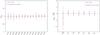 |
Fig. 1 In this figures we plot the values of the difference, Δ, between spectral features in the observed and model spectra, averaged over all the spectra of the wings sample with an acceptable spectral fit (χ2 < 3). On the left panel we show the differences calculated for the continuum flux (both observed and model spectra have been normalized to 1 at 5500 Å), and on the right panel for the equivalent width of the lines. Red points represent the average value of Δ, for each one of the continuum bands and emission lines that were used as constraints in the fit. The red errorbars are the corresponding rms, while blue ones are the average of the observed rms. |
As we describe in F07, this set of theoretical spectra originally included also a SSP whose age, namely ~17.5 Gyr, is older than the universe age. The use of this SSP was merely statistical: since the only appreciable difference between the three oldest SSPs of our set is, actually, the mass-to-luminosity ratio, using such an old SSP would prevent our random search of the best fit model to be systematically biased towards the youngest of the old SSPs. Nevertheless, the adoption of such an approach can lead some models to be dominated by this very old stellar population yielding, in this way, mass values that are too high, due to the higher mass-to-light ratio. To overcome this issue we decide to avoid the use of the oldest stellar populations, limiting ourselves to stellar populations whose ages are consistent with that of the universe. We will hence refer, from now on, to these 12 SSPs.
3.3. The best fit search
Finding the best combination of the parameters that minimizes the differences between the observed and the model spectrum, is a non-linear problem, due to the presence of extinction. Furthermore, it is also underdetermined, which means that the number of constraints is lower than the number of parameters. In fact, in our case, we are using SSPs of 12 different ages, so that our task turns into finding the combination of 12 mass and extinction values that better fits the observed spectrum. To find the set of 24 parameters that will yield the best fit model, we use the Adaptive Simulated Annealing algorithm, which randomly explores the parameters space, searching for an absolute minimum in the χ2 function. This method is particulary suited to such problems, where the function to minimize has lots of local minima: once a promising zone for a minimum, in the parameter space, is found, the algorithm not only refines the search of the local minimum, but also checks for the presence of other, deeper minima, outside the local “low-χ2 valley”.
3.4. Uncertainties
All the physical parameters that are derived from the the spectral analysis, refer to a best fit model for an observed spectrum. The limited wavelength range under analysis, the well known age-metallicity degeneracy, and the non-linearity of the problem, together with the fact that it is underdetermined, makes the solution non-unique. This means that models with different characteristics may equally well reproduce the observed spectral features. To account for this, we give error-bars related to mass, extinction and age values.
To compute such uncertainties, we exploit the characteristics of the minimisation algorithm: the path towards the best fit model (or the minimum χ2) depends on the starting points so, in general, starting from different initial positions can lead to different minimum points, i.e. to best fit models with different parameters. We hence perform 11 optimisations, each time starting from a different point in the parameters space. In this way we end up with 11 best fit models that we verified are well representative of the space of the solutions. We take, as a reference, the model with the median total mass among these 11. All the errorbars are computed as the average difference between the values of the models with the highest and lowest total stellar mass.
3.5. The quality of the fits
The similarity between an observed spectrum and its best fit model is measured, as explained in Sect. 3.1, by means of a χ2 function taking into account both spectral continuum fluxes and the equivalent widths of significant lines. Our choice to use a wide range both in metallicity and SSP ages, and to let both extinction and mass vary freely, are the key ingredients that allow us to satisfactorily reproduce any galactic spectrum, at least in principle.
In practice, low quality spectra due to low S / N, bad flux calibration, bad subtraction of sky or telluric lines, can give rise to a bad fit. To demonstrate that there are no systematic failures of any of the observed features that are used as constraints, in Fig. 1 we show the difference between the values calculated for the model and for the observed spectrum, averaged over all the wings sample. In the left-hand panel we show, plotted as red squares, the average values of the difference for the flux in the spectral continuum, together with the rms (red errorbars), and the average values of the observed errors (blue errorbars).
The plot in the right-hand panel of the same figure shows the differences for the equivalent widths of the spectral lines. The [Oii] line is the one that shows the highest displacement with respect to the zero-difference line, due to the fact that this line is in the spectral region with the highest noise. This makes it also more difficult to measure, and it also explains why its observed value has the average largest error. Overall all the features are well reproduced, with no systematic failure.
4. The properties of stellar populations
In this section we describe the properties of the stellar populations that are derived from our spectrophotometric synthesis, that are now publicly available. Fitting the main features of an optical spectrum allows us to derive the characteristics of the stellar populations whose light we see in the integrated spectrum: total mass, mass of stars as a function of age, the metallicity and dust extinction are typical quantities that can be obtained. As already pointed out, using this particular technique, it is almost impossible to recover a unique value for the stellar metallicity due to both the degeneracy issues such as the age-metallicity and age-extinction and to the fact that we do not consider SSP models with α-element enhancements. In fact, in the vast majority of cases at least two values of the metallicity are found to provide equally good fits.
4.1. Stellar masses
When stellar masses are derived by means of spectrophotometric techniques, it is important to clearly state which definition of mass is used. As already made clear by Longhetti & Saracco (2009, but see also Renzini 2006), the use of spectral synthesis techniques leads to three different definitions of the stellar mass, namely:
-
1.
the initial mass of the SSP, at age zero; this isnothing but the mass of gas turned into stars;
-
2.
the mass locked into stars, both those which are still in the nuclear-burning phase, and remnants such as white dwarfs, neutron stars and stellar black holes;
-
3.
the mass of stars that are still shining, i.e. in a nuclear-burning phase.
The difference between the three definitions is a function of the stellar age and, in particular, it can be up to a factor of 2 between mass definition 1) and 3), in the oldest stellar populations. We will provide the user with masses calculated using all of the afore mentioned definitions, following the same enumeration.
To compute the values of stellar mass, we exploit the fact that the theoretical spectra are given in luminosity per unit of solar mass. Once the model spectrum is converted to flux by accounting for the luminosity distance factor, the K-correction is naturally performed by fitting the spectra at their observed redshifts. All of the observed spectra are normalised by means of their observed V-band magnitude within the fiber aperture. Obviously, in order to obtain a stellar mass value referring to the whole galaxy (that we will dub “total stellar mass”, from now on), one should use a spectrum representative of the whole galaxy, which is not at our disposal. Since we have both aperture and total photometry for all the objects of our spectroscopic sample, we use the total V magnitude to rescale the model spectrum: in this way we are assuming that the colour gradient of the aperture-to-total magnitude is negligible (this assumption is made by several authors: see e.g. Kauffmann et al. 2003). When speaking of “total magnitude” here, we refer to the MAG_AUTO value (see Varela et al. 2009, for further details), that is the SExtractor magnitude computed within the Kron aperture.
In Fig. 2 we show the comparison between the observed (B − V) colour computed using the magnitudes within a 5 kpc aperture (x axis) an the one computed using the spectroscopic fiber aperture (y axis), with the black line being the 1:1 relation. We consider the color within 5 kpc a good approximation of the total color (in fact, it closely follows the color derived using AUTO magnitudes), and is a good aperture compromise for both large and small galaxies in our sample. The average difference between the fibre and 5 kpc colours is ~0.1 mag, due to the presence of bluer (thus probably younger) stars in the outskirts of the galaxies. We will provide values of the stellar mass referring to both apertures, and a colour term which can be used to correct the total mass to account for radial gradients in the stellar populations content, as described below.
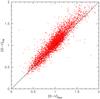 |
Fig. 2 The comparison between values of the (B − V) colour as computed from a 5 kpc aperture (x axis) and the fiber aperture (y axis) magnitudes. The solid line represents the 1:1 relation that highlights a systematic, off-set of ~0.1 mag: the 5 kpc colour is bluer as expected since the total magnitude is sampling, on average, younger populations in the outskirts of the galaxies. |
4.2. Colour corrections
To correct total masses for colour gradients, we exploit the Bell & de Jong (2001) prescription, which was derived in order to compute stellar masses in galaxies by means of photometric data. According to their work, the M / L ratio of a galaxy can be expressed by the following:  (2)where Lλ is the luminosity in a given band (denoted by λ) while the aλ and bλ coefficients depend on the band that is used, and on the population synthesis models (including IMF, isochrones, etc.), and COL is the colour term. Table 4 in Bell & de Jong (2001) presents a list of such coefficients for various bands, models and two metallicities (subsolar – Z = 0.008 – and solar – Z = 0.02 –). For the calculations that follow, we will use V and B band data, and assume the Kodama & Arimoto (1997) models, that use a Salpeter IMF and a solar metallicity value, which yields aV = −0.18 and bV = 1.00. Note that, using Bruzual & Charlot (2003) or pegase (Fioc & Rocca-Volmerange 1997) models, will not substantially affect the results.
As already mentioned above, when going from the stellar mass calculated over the fiber magnitude to the one referring to the whole galaxy, there is the implicit assumption that the colour calculated within the fiber aperture is the same as the one calculated with the total magnitudes (here we assume a ~5 kpc aperture), while this is not true for most cases. Starting from Eq. (2) and after some algebra, we derive a colour-correction term as follows: ![Mathematical equation: \begin{equation} \label{eqn:ccol} C_{\rm corr}= b_V\cdot [(B_5-V_5)-(B_f-V_f)] \end{equation}](/articles/aa/full_html/2011/02/aa15214-10/aa15214-10-eq53.png) (3)where the term (B5 − V5) is the colour computed from 5 kpc aperture magnitudes and (Bf − Vf) is the observed colour within the fiber. This factor, which is given in our final catalogs, must be added to the total mass value in order to account for colour gradients.
(3)where the term (B5 − V5) is the colour computed from 5 kpc aperture magnitudes and (Bf − Vf) is the observed colour within the fiber. This factor, which is given in our final catalogs, must be added to the total mass value in order to account for colour gradients.
As a consistency check for the values of the total stellar mass computed by means of our models, we compare them to the values that can be obtained by means of Eq. (2), which yields the following: 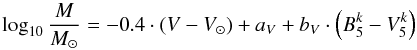 (4)where
  are the K-corrected (i.e. rest-frame) magnitudes extracted from a 5 kpc aperture, V is the total absolute magnitude (obtained from V MAG_AUTO, K-corrected) and V⊙ = 4.82 is the absolute magnitude of the sun in the V band. K-corrections were taken from Poggianti (1997).
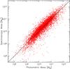 |
Fig. 3 A comparison of the total stellar mass of galaxies in the wings sample, as computed by means of B and V band photometry, on the x-axis, assuming the prescriptions given in (Bell & de Jong 2001, see text for details), and by means of our spectral fitting. The solid line represents the 1:1 relation. A colour correction term, computed as explained in the text, was applied to the spectroscopic-derived values, while the photometric values were corrected to account for the difference in the IMF mass limits. |
In Fig. 3 we show the comparison between total stellar masses computed by means of our spectral fitting (on the y-axis) and those obtained by means of the Bell & de Jong (2001) prescription (i.e. by adopting Eq. (4)). We applied a 0.064 dex correction to account for the differences in the adopted IMF (Bell & de Jong 2001, use a Salpeter IMF with masses in the 0.1–100 M⊙ range, while we use 0.15–120 M⊙), and we added the colour correction term to the spectroscopic-derived mass values, as explained above. The agreement between the two different methods is, on average, always better than 0.1 dex. A similar comparison between stellar masses obtained from spectral fitting and from photometry, calculated using aperture magnitudes instead of the total ones, shows an equally good agreement between the two methods. The Bell & de Jong (2001) mass photometric values are also provided in our final catalogs.
4.3. The star formation history
As we describe in F07 and summarize in Sect. 3.2, our search for the best fit-model is performed using 12 SSPs of different ages, obtained, in turn, by binning a much higher age-resolution stellar age grid. Still, we verified that it is not possible to recover the star formation as a function of stellar age with the relatively high temporal resolution provided by the 12 SSPs. After performing accurate tests on template spectra that were built in order to match the spectral features of wings spectra in terms of both spectral resolution, signal-to-noise ratio and wavelength coverage, we found that it is possible to properly recover the star formation history (hereafter, SFH) in 4 main stellar age bins. The details of the choice are explained in F07; here we just recall their ranges that are, respectively: 0−2 × 10⁷, 2 × 10⁷−6 × 10⁸, 6 × 10⁸−5.6 × 10⁹ and 5.6 × 10⁹−14 × 109 years.
The SFH is given in our catalogs in two different forms: 1) percentage of the stellar mass and 2) star formation rate (SFR) in the four bins. The first is computed according to the following: 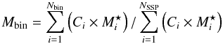 (5)where Nbin is the number of SSPs contained in a given age bin; Ci is the normalisation constant of each SSP of that bin, i.e. the stellar mass at each age according to definition 1;
  is the factor, which is a function of the stellar age, that converts the SSP initial mass (definition 1.) into either the mass locked into stars (mass definition 2.) or into mass of nuclear burning stars (definition 3.), while the sum at the denominator is the total stellar mass (according to definitions 2 and 3, respectively).
The star formation rate as a function of the stellar age is computed by dividing the stellar mass of a given age bin by its duration. Definition 1 of the mass was applied in this calculation (see also Eq. (1) in Longhetti & Saracco 2009).
The current SFR value, i.e. the one calculated within the youngest age bin, deserves a particular attention, since it is calculated by fitting the equivalent width of emission lines, namely Hydrogen (Hα and Hβ) and Oxygen ([Oii] at 3727 Å). The lines’ luminosity is entirely attributed to star formation processes neglecting other mechanisms that can produce ionizing flux. In this way we are overestimating the current SFR in both LINERS and AGNs. In a forthcoming work, we will present an analysis of standard diagnostic diagrams such as those by Veilleux & Osterbrock (1987), with the lines’ intensities accurately measured by subtracting stellar templates from the observed spectrum (Marziani et al., in prep.). This work will enable the distinction between “pure” star forming systems and those where other mechanisms might be co-responsible for line emission.
4.4. Dust extinction
According to the “selective extinction” hypothesis (Calzetti et al. 1994), which we fully consider in our modelling, each SSP has its own value of the dust attenuation. We compute an age-averaged value of dust extinction, as it is derived by the model, by using Eq. (6): ![Mathematical equation: \begin{equation} \label{eqn:av} A_V=-2.5\times \log_{10}\left[\frac{L_{\rm tot}^{\rm M}(5550)}{L_{\rm unext}^M(5550)} \right] \end{equation}](/articles/aa/full_html/2011/02/aa15214-10/aa15214-10-eq67.png) (6)where
(6)where  and
and  are, respectively, the model spectrum and the model non-attenuated spectrum (i.e. the model with the same SFH as
  but with AV = 0 for each stellar population). We calculate two distinct values: we first take into account only stellar populations that are younger than ~2 × 10⁷, i.e. those that are responsible for nebular emission; this value is comparable with extinction that is computed from emission lines ratio. Secondly, we use all stellar populations providing, in this way, an extinction value which is averaged over SSP of all ages.
4.5. Average ages
Exploiting the information derived by our analysis, we are able to provide an estimate of the average age of a galaxy, weighted on the stellar populations that compose its spectrum. Given that the mass-to-light ratio changes as a function of the age, there are two different definitions that can be given: the mass-weighted and the luminosity-weighted age (see also Fernandes et al. 2003). The latter is the most commonly given, since it is directly derived from the spectrum, being weighted in this way towards the age of the stellar populations that dominate the light, while the first definition requires the knowledge of the mass distribution as a function of stellar age, i.e. the SFH. We can compute the logarithm of these two quantities as follows: 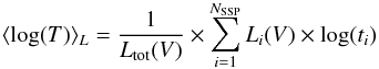 (7)for the logarithm of the luminosity weighted age, where Li(V) and Ltot(V) are the restframe luminosities of the ith SSP and of the total spectrum, respectively, in the V-band, and ti the age of the ith SSP. The mass-weighted age is computed in a similar way as:
  (8)and, similarly, Mtot and Mi are the total mass and the mass of the ith SSP, respectively. Hence, while the luminosity-weighted age gives an estimate of the age of stars that dominate the optical spectrum, being in this way more sensitive to the presence of young stars, the mass-weighted value is more representative of the actual average age of a galaxy’s stellar populations. Note that to compute these values, we use the finest age grid, averaging over the 12 stellar populations.
We provide both the luminosity-weighted age computed from the V-band, and the one computed from the bolometric luminosity. The two values are, anyway, very similar.
4.6. Absolute magnitude computation and prediction
The fact that the theoretical SSP spectra that we use for our modeling cover a wide range in wavelengths, allows us to compute absolute magnitudes in various bands that are not covered by the observed spectra, without having to assume any K-correction. To compute the absolute magnitude of a galaxy, we take the best-fit model spectrum, compute its flux as if it was observed at 10 pc and convolve it with the proper filter transmission curve:  (9)where Tb(λ) is the transmission curve of the filter for the band b and
  is the model spectrum calculated at a distance of 10 pc. For the sake of clearity, in Table 1 we provide the zero-point fluxes, expressed in erg/s/cm2/Å that were used to compute all of the magnitudes. UBVRIJHK magnitudes are computed according to the Johnson system, while ugriz magnitudes are calculated in order to match the Sloan system.
Zero-point fluxes used to calculate observed expected magnitudes and absolute magnitudes, together with their effective lambda.
5. Validation
In order to compare with the widely used sdss masses, we performed a comparison of the stellar mass values for a subsample of wings galaxies that has been spectroscopically observed also by the sdss. As a reference for masses from the SLOAN survey we used those derived by Gallazzi et al. (2005), using the Data Release 4 (DR4)12, and those obtained from the photometry exploiting Data Release 7 (DR7)2. In this way, we built two sub-samples of galaxies observed by both surveys, namely 395 in the wings-DR4 sample, and 606 in the wings-DR7 sample.
Example of entries in the SFH catalog.
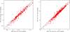 |
Fig. 4 In the left panel we show the comparison between mass values that we obtained by fitting sdss spectra with our model, and those calculated by Gallazzi et al. (2005). The black line represents the 1:1 relation and the blue dotted-dashed line is the least-square fit to the data. On the right, we compare mass values we derived using our spectrophotometric fitting on the sloan’s fiber spectrum, to those obtained from DR7 photometric data fitting, referring to the same aperture. Lines and symbols as in the left panel. All sets of mass values have been corrected to account for differences in the assumed IMF (see text for details), and those that are shown here are normalized to the Kroupa (2001) IMF. |
We performed a double check: as a first step, we exploited our spectrophotometric model to derive, using sdss spectra and g (model-)band magnitudes of the wings-DR4 sample, the same quantities that were inferred for wings galaxies. In this way, comparing the results obtained with the same (sdss) data but with different methods, we can demonstrate the reliability of our technique. As a second step, we compare total stellar mass values obtained with our model and wings data, to those of the sdss DR4 and DR7, respectively.
To ensure this comparison is significant, we have to consider the details of the models used to derive such quantities. In particular, we have to take into account the differences in the IMFs that are assumed, i.e. Salpeter (1955) for wings (we recall here that the mass limits that we have adopted are 0.15 and 120 M⊙, respectively), Chabrier (2003) for masses derived by Gallazzi et al. (2005), and Kroupa (2001) for sdss, DR7, respectively. We have determined that the difference between Salpeter’s and Kroupa’s IMF is a factor of ~1.33 (0.125 dex), the Salpeter IMF yielding the highest values of masses, while Chabrier’s IMF yields stellar masses that are 1.1 (0.04 dex) times lower with respect to Kroupa’s (see, e.g., Cimatti et al. 2008). For the sake of homogeneity, and only for the purposes of these sanity checks, we will rescale all the mass values to the Kroupa (2001) IMF. Note that all the mass values we refer to are calculated according to definition 2. (see Sect. 4.1).
In Fig. 4 we show how the different methods compare, exploiting both DR4 and DR7 data. In the left-hand panel, we plot mass values derived using our model against those obtained by Gallazzi et al. (2005), both from sdss DR4 data. Our mass determination was obtained by fitting the sdss spectrum – which was normalized to the total model g band magnitude – in the same way as done for wings data. The agreement between the two methods overall is good, with an rms of ~0.21.
In the right-hand panel of Fig. 4 we show the comparison between the masses we derived from the sdss spectroscopy scaled to the g band fiber magnitude and the fiber-aperture photometric masses from the DR7. Hence, we are comparing two mass estimates within the same fibre aperture, obtained using either the sdss spectroscopy+photometry or only sdss photometry, and we do not have to deal with aperture effects. The rms is ~0.17, but it is worth noting that, the data displays a ~0.15 dex systematic offset, in the sense that the DR7 yields slightly lower masses. This is in contrast to the DR4 comparison which shows remarkable agreement, even though there is some dispersion with respect to the 1:1 relation. A small offset in the same direction is present also when comparing DR4 and DR7 masses for galaxies in common, as shown in Fig. 5.
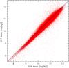 |
Fig. 5 The comparison between total mass values from the sdss DR4, as calculated by Gallazzi et al. (2005), and those obtained from DR7 photometry. Both masses are rescaled to a Kroupa (2001) IMF. |
In Fig. 6 we move to the comparison of the total stellar masses we derived from the wings data, corrected for color gradients, and total masses given by Gallazzi et al. (2004) and DR7, always considering galaxies of the subsamples in common. The scatter around the 1:1 relation is slightly larger in these cases, (0.23 and 0.22 for DR4 and DR7, respectively) and for the DR7-derived masses the average difference is negligible at low masses and tends to increase with mass. For this comparison, in addition to the different mass estimate methods, the data are also different: wings spectra are taken within an aperture of ~2″ while Sloan fibers cover a ~3″ aperture, centered on a position that can be, in general, different. Also, source and flux extraction techniques, and the spectral resolution of the two surveys are different. The general agreement, however, is satisfactory, and the scatter is similar to the ~0.2 dex accuracy expected with these methods (e.g. Cimatti et al. 2008).
We conclude that, despite the substantial differences in the fitting approach, in the adopted theoretical libraries and in the characteristics of the datasets themselves, our total mass values are in overall agreement with those of a considerable number of objects that the sdss has in common with wings.
Description of items of the SFH catalog.
6. The catalogs
In this section we briefly describe the most relevant quantities given in the catalogs we are releasing to the astronomical community. About 70% of the observed spectra have been fitted with a χ2 ≤ 3 and we consider fits with such values to be reliable. For higher values, a visual inspection is recommended to asses the reliability of the spectral fit.
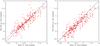 |
Fig. 6 In the left panel we show the comparison between mass values from the sdss DR4, as calculated by Gallazzi et al. (2005), and those obtained by means of our spectrophotometric model on wings spectra and magnitudes. On the right panel we present the same comparison, but with DR7 masses, derived from total magnitude. The large scatter is due to the combination of both different methods and different data. The black line is the 1:1 relation, and the red line is the least-square fit to the data for both plots. All the values are rescaled to the Kroupa (2001) IMF, and a colour correction term has also been applied to wings masses (see Sect. 4.2). |
For each spectrum that has been analyzed we give the following:
-
the reduced χ2 for the fits obtained for the three values of metallicity. Note that we take as a reference model the one with the value of the metallicity that yields the lowest χ2 value, regardless of the fact that other values of the metallicity are also providing acceptable fits. These values are also useful to flag potentially unreliable fits. A χ2 ≤ 3 can be used as a discriminant for blindly accepting a result;
-
extinction in the V band, in magnitudes, computed from the model spectrum both averaging on young stellar populations (i.e. with age ≤ 2 × 10⁷ years) and on all ages, including uncertainties on both quantities;
-
SFR in the four main age bins as defined in Sect. 4.3, with related uncertainties, all expressed in M⊙ / yr; note that these SFRs only refer to values normalized to the fiber-aperture magnitude. In order to compute the global value, one should multiply the fiber-SFR by a factor ℘ = 10−0.4·(Vtot − Vfib), that is the ratio of total and aperture fluxes;
-
percentage of the stellar mass in the 4 main age bins, with related uncertainties, calculated for the different mass definitions;
-
the logarithm of total stellar mass, expressed in M⊙, within the fiber aperture, according to the 3 definitions explained in Sect. 4.1, together with the related uncertainties (expressed in logarithm of solar masses as well), which are computed for the definition 3;
-
the logarithm of total stellar mass, expressed in M⊙, computed by rescaling the fiber spectrum to the total V magnitude (see Sect. 4.1), and the related uncertainties (in logarithm of the solar mass), uncorrected for color gradients;
-
the logarithm of the stellar mass calculated from the B and V band photometry, according to the Bell & de Jong (2001) prescription, for both total and fiber magnitudes;
-
the colour–correction term, described in Sect. 4.2, to be added to the total mass to account for colour gradients;
-
the logarithm of the luminosity-weighted age computed both using the luminosity in the V band, and the bolometric emission, and the related uncertainties: the latter are computed only with respect to the bolometric luminosity-weighted age;
-
the logarithm of the mass-weighted age, and the related uncertainty;
-
Galactic extinction-corrected observed B and V magnitude referring to both the fiber and the total aperture; we report these magnitudes even though they are actually measured values (see Varela et al. 2009), because these are the values used to rescale the observed spectrum and, hence, to derive the total mass. Values of extinction within our Galaxy for each of the clusters were taken from NED (see also Schlegel et al. 1998);
-
absolute V and B magnitudes calculated from the observed spectrum, derived from both aperture and total magnitudes;
-
Johnson (UBVIRJHK) and Sloan (ugriz) expected observed magnitudes calculated from our best model spectrum, both within our fiber aperture and total;
-
Johnson (UBVIRJHK) and Sloan (ugriz) absolute magnitudes calculated from our best model spectrum, both within our fiber aperture and total.
Whenever one of the above listed quantities is not available, this is flagged with a 99.99.
All the data and physical quantities described in this paper will be available by querying the wings database at the following web address: http://web.oapd.inaf.it/wings/.
In Table 2 we give an example of how the full set of information will look like, reporting data for 5 galaxies of the sample. A description of each item, together with their units, can be found in Table 3, where we report, respectively: the column ID in the catalog, the item’s name as it appears in the database, its format, physical units and description.
Please refer to the wings website for updated details about both the survey and its products; http://web.oapd.inaf.it/wings/new/index.html
Stellar masses computed by Gallazzi et al. (2005), by means of DR4 data are publicly available at this website: http://www.mpa-garching.mpg.de/SDSS/DR4/Data/stellarmet.html
Stellar mass values for the DR7 data release were taken from the following sdss website: http://www.mpa-garching.mpg.de/SDSS/DR7/Data/stellarmass.html
Acknowledgments
This paper took great advantage from discussions with Anna Gallazzi and Jarle Brinchmann, who kindly provided us with all the details of their stellar masses calculations using DR4 and DR7, respectively. Funding for the SDSS and SDSS-II has been provided by the Alfred P. Sloan Foundation, the Participating Institutions, the National Science Foundation, the U.S. Department of Energy, the National Aeronautics and Space Administration, the Japanese Monbukagakusho, the Max Planck Society, and the Higher Education Funding Council for England. The SDSS Web Site is: http://www.sdss.org/. We are grateful to the anonymous referee, whose comments and remarks helped us to improve the quality and the readability of this work.
References
- Bell, E. F., & de Jong, R. S. 2001, ApJ, 550, 212 [NASA ADS] [CrossRef] [Google Scholar]
- Bertelli, G., Bressan, A., Chiosi, C., Fagotto, F., & Nasi, E. 1994, A&AS, 106, 275 [NASA ADS] [Google Scholar]
- Bressan, A., Granato, G. L., & Silva, L. 1998, A&A, 332, 135 [NASA ADS] [Google Scholar]
- Bruzual, A. G. 1983, ApJ, 273, 105 [NASA ADS] [CrossRef] [Google Scholar]
- Bruzual, G., & Charlot, S. 2003, MNRAS, 344, 1000 [NASA ADS] [CrossRef] [Google Scholar]
- Calzetti, D., Kinney, A. L., & Storchi-Bergmann, T. 1994, ApJ, 429, 582 [NASA ADS] [CrossRef] [Google Scholar]
- Cardelli, J. A., Clayton, G. C., & Mathis, J. S. 1989, ApJ, 345, 245 [NASA ADS] [CrossRef] [Google Scholar]
- Cava, A., Bettoni, D., Poggianti, B. M., et al. 2009, A&A, 495, 707 [NASA ADS] [CrossRef] [EDP Sciences] [Google Scholar]
- Chabrier, G. 2003, ApJ, 586, L133 [NASA ADS] [CrossRef] [Google Scholar]
- Cimatti, A., Cassata, P., Pozzetti, L., et al. 2008, A&A, 482, 21 [NASA ADS] [CrossRef] [EDP Sciences] [Google Scholar]
- Dressler, A., Oemler, A., Jr.,Couch, W. J., et al. 1997, ApJ, 490, 577 [NASA ADS] [CrossRef] [Google Scholar]
- Fasano, G., Marmo, C., Varela, J., et al. 2006, A&A, 445, 805 [NASA ADS] [CrossRef] [EDP Sciences] [Google Scholar]
- Ferland, G. J. 1996, Hazy, a Brief Introduction to CLOUDY, in University of Kentucky, Department of Physics and Astronomy Internal Report [Google Scholar]
- Fernandes, R. C., Leão, J. R. S., & Lacerda, R. R. 2003, MNRAS, 340, 29 [NASA ADS] [CrossRef] [Google Scholar]
- Fioc, M., & Rocca-Volmerange, B. 1997, A&A, 326, 950 [NASA ADS] [Google Scholar]
- Fritz, J., Poggianti, B. M., Bettoni, D., et al. 2007, A&A, 470, 137 [NASA ADS] [CrossRef] [EDP Sciences] [Google Scholar]
- Fukugita, M., Ichikawa, T., Gunn, J. E., et al. 1996, AJ, 111, 1748 [NASA ADS] [CrossRef] [Google Scholar]
- Gallazzi, A., Charlot, S., Brinchmann, J., White, S. D. M., & Tremonti, C. A. 2005, MNRAS, 362, 41 [NASA ADS] [CrossRef] [Google Scholar]
- Jacoby, G. H., Hunter, D. A., Christian, C. A. 1984, ApJS, 56, 257 [NASA ADS] [CrossRef] [Google Scholar]
- Kauffmann, G., Heckman, T. M., White, S. D. M., et al. 2003, MNRAS, 341, 33 [NASA ADS] [CrossRef] [Google Scholar]
- Kodama, T., & Arimoto, N. 1997, A&A, 320, 41 [NASA ADS] [Google Scholar]
- Kroupa, P. 2001, MNRAS, 322, 231 [NASA ADS] [CrossRef] [Google Scholar]
- Longhetti, M., & Saracco, P. 2009, MNRAS, 394, 774 [NASA ADS] [CrossRef] [Google Scholar]
- Moro, D., & Munari, U. 2000, A&AS, 147, 361 [NASA ADS] [CrossRef] [EDP Sciences] [Google Scholar]
- Osterbrock, D. E. 1989, Research supported by the University of California, John Simon Guggenheim Memorial Foundation, University of Minnesota, et al. Mill Valley, CA, University Science Books, 422 [Google Scholar]
- Poggianti, B. M. 1997, A&AS, 122, 399 [NASA ADS] [CrossRef] [EDP Sciences] [Google Scholar]
- Poggianti, B. M., Smail, I., Dressler, A., et al. 1999, ApJ, 518, 576 [NASA ADS] [CrossRef] [Google Scholar]
- Poggianti, B. M., Desai, V., Finn, R., et al. 2008, ApJ, 684, 888 [NASA ADS] [CrossRef] [Google Scholar]
- Postman, M., & Geller, M. J. 1984, ApJ, 281, 95 [NASA ADS] [CrossRef] [Google Scholar]
- Postman, M., Franx, M., Cross, N. J. G., et al. 2005, ApJ, 623, 721 [NASA ADS] [CrossRef] [Google Scholar]
- Renzini, A. 2006, ARA&A, 44, 141 [NASA ADS] [CrossRef] [Google Scholar]
- Salpeter, E. E. 1955, ApJ, 121, 161 [Google Scholar]
- Sánchez-Blázquez, P. 2004, Ph.D. Thesis, [Google Scholar]
- Sánchez-Blázquez, P., Peletier, R. F., Jiménez-Vicente, J., et al. 2006, MNRAS, 371, 703 [NASA ADS] [CrossRef] [Google Scholar]
- Schlegel, D. J., Finkbeiner, D. P., & Davis, M. 1998, ApJ, 500, 525 [NASA ADS] [CrossRef] [Google Scholar]
- Valentinuzzi, T., Woods, D., Fasano, G., et al. 2009, A&A, 501, 851 [NASA ADS] [CrossRef] [EDP Sciences] [Google Scholar]
- Varela, J., D’Onofrio, M., Marmo, C., et al. 2009, A&A, 497, 667 [NASA ADS] [CrossRef] [EDP Sciences] [Google Scholar]
- Veilleux, S., & Osterbrock, D. E. 1987, ApJS, 63, 295 [NASA ADS] [CrossRef] [Google Scholar]
All Tables
Zero-point fluxes used to calculate observed expected magnitudes and absolute magnitudes, together with their effective lambda.
All Figures
|
Fig. 1 In this figures we plot the values of the difference, Δ, between spectral features in the observed and model spectra, averaged over all the spectra of the wings sample with an acceptable spectral fit (χ2 < 3). On the left panel we show the differences calculated for the continuum flux (both observed and model spectra have been normalized to 1 at 5500 Å), and on the right panel for the equivalent width of the lines. Red points represent the average value of Δ, for each one of the continuum bands and emission lines that were used as constraints in the fit. The red errorbars are the corresponding rms, while blue ones are the average of the observed rms. |
| In the text | |
|
Fig. 2 The comparison between values of the (B − V) colour as computed from a 5 kpc aperture (x axis) and the fiber aperture (y axis) magnitudes. The solid line represents the 1:1 relation that highlights a systematic, off-set of ~0.1 mag: the 5 kpc colour is bluer as expected since the total magnitude is sampling, on average, younger populations in the outskirts of the galaxies. |
| In the text | |
|
Fig. 3 A comparison of the total stellar mass of galaxies in the wings sample, as computed by means of B and V band photometry, on the x-axis, assuming the prescriptions given in (Bell & de Jong 2001, see text for details), and by means of our spectral fitting. The solid line represents the 1:1 relation. A colour correction term, computed as explained in the text, was applied to the spectroscopic-derived values, while the photometric values were corrected to account for the difference in the IMF mass limits. |
| In the text | |
|
Fig. 4 In the left panel we show the comparison between mass values that we obtained by fitting sdss spectra with our model, and those calculated by Gallazzi et al. (2005). The black line represents the 1:1 relation and the blue dotted-dashed line is the least-square fit to the data. On the right, we compare mass values we derived using our spectrophotometric fitting on the sloan’s fiber spectrum, to those obtained from DR7 photometric data fitting, referring to the same aperture. Lines and symbols as in the left panel. All sets of mass values have been corrected to account for differences in the assumed IMF (see text for details), and those that are shown here are normalized to the Kroupa (2001) IMF. |
| In the text | |
|
Fig. 5 The comparison between total mass values from the sdss DR4, as calculated by Gallazzi et al. (2005), and those obtained from DR7 photometry. Both masses are rescaled to a Kroupa (2001) IMF. |
| In the text | |
|
Fig. 6 In the left panel we show the comparison between mass values from the sdss DR4, as calculated by Gallazzi et al. (2005), and those obtained by means of our spectrophotometric model on wings spectra and magnitudes. On the right panel we present the same comparison, but with DR7 masses, derived from total magnitude. The large scatter is due to the combination of both different methods and different data. The black line is the 1:1 relation, and the red line is the least-square fit to the data for both plots. All the values are rescaled to the Kroupa (2001) IMF, and a colour correction term has also been applied to wings masses (see Sect. 4.2). |
| In the text | |
Current usage metrics show cumulative count of Article Views (full-text article views including HTML views, PDF and ePub downloads, according to the available data) and Abstracts Views on Vision4Press platform.
Data correspond to usage on the plateform after 2015. The current usage metrics is available 48-96 hours after online publication and is updated daily on week days.
Initial download of the metrics may take a while.