| Issue |
A&A
Volume 526, February 2011
|
|
|---|---|---|
| Article Number | A51 | |
| Number of page(s) | 14 | |
| Section | Extragalactic astronomy | |
| DOI | https://doi.org/10.1051/0004-6361/201014968 | |
| Published online | 21 December 2010 | |
A possible jet precession in the periodic quasar B0605–085
1
Max-Planck-Institut für Radioastronomie,
Auf dem Hügel 69,
53121
Bonn,
Germany
e-mail: This email address is being protected from spambots. You need JavaScript enabled to view it.
2
Physics Department, University College Cork,
Cork,
Ireland
3
Astronomical Institute of St. Petersburg State University,
Universitetskiy Prospekt 28, Petrodvorets
198504, St. Petersburg,
Russia
4
Departament d’Astronomia i Astrofìsica, Universitat de
València, 46100
Burjassot, València, Spain
5
Astronomy Department, University of Michigan,
Ann Arbor, MI
48109,
USA
6
Metsähovi Radio Observatory, TKK, Helsinki University of
Technology, Metsähovintie
114, 02540
Kylmälä,
Finland
7
I. Physikalisches Institut, Universität zu Köln,
Zülpicher Str. 77,
50937
Köln,
Germany
Received:
10
May
2010
Accepted:
6
July
2010
Abstract
Context. The quasar B0605−085 (OH 010) shows a hint for probable periodical variability in the radio total flux-density light curves.
Aims. We study the possible periodicity of B0605−085 in the total flux-density, spectra, and opacity changes in order to compare it with jet kinematics on parsec scales.
Methods. We have analyzed archival total flux-density variabilities at ten frequencies (408 MHz, 4.8 GHz, 6.7 GHz, 8 GHz, 10.7 GHz, 14.5 GHz, 22 GHz, 37 GHz, 90 GHz, and 230 GHz) together with the archival high-resolution very long baseline interferometry data at 15 GHz from the MOJAVE monitoring campaign. Using the Fourier transform and discrete autocorrelation methods we have searched for periods in the total flux-density light curves. In addition, spectral evolution and changes of the opacity have been analyzed.
Results. We found a period in multi-frequency total flux-density light curves of 7.9 ± 0.5 yrs. Moreover, a quasi-stationary jet component C1 follows a prominent helical path on a similar timescale of eight years. We have also found that the average instantaneous speeds of the jet components show a clear helical pattern along the jet with a characteristic scale of 3 mas. Taking into account average speeds of jet components, this scale corresponds to a timescale of about 7.7 years. Jet precession can explain the helical path of the quasi-stationary jet component C1 and the periodical modulation of the total flux-density light curves. We have fitted a precession model to the trajectory of the jet component C1, with a viewing angle φ0 = 2.6° ± 2.2°, aperture angle of the precession cone Ω = 23.9° ± 1.9° and fixed precession period (in the observers frame) P = 7.9 yrs.
Key words: galaxies: active / galaxies: jets / radio continuum: galaxies / quasars: general / quasars: individual: B0605 − 085
Member of the International Max Planck Research School (IMPRS) for Astronomy and Astrophysics.
© ESO, 2010
1. Introduction
The radio source B0605−085 (OH 010) is a quasar that is very bright at centimeter and millimeter wavelengths with a redshift of 0.872 (Stickel et al. 1993). B0605−085 was studied in X-ray and optical wavelengths with the CHANDRA and HST telescopes by Sambruna et al. (2004) and is one of a few quasars whose jets have been detected in the X-rays. Very Long-Baseline Interferometry (VLBI) observations revealed a complex structure of the radio jet of the quasar, with multiple bends and curves at scales from parsecs to kiloparsecs. High-resolution space VLBI observations show that the inner jet extends in the southeast direction and at ~0.2 mas it turns to the northeast (Scott et al. 2004). When observed at centimeter wavelengths, the outer part of the jet continues to extend southeast with multiple turns, and at kilo-parsec scales it goes eastwards with a southeast bend at ~3 arcsec (Cooper et al. 2007). The kinematics of the B0605−085 jet was studied by Kellermann et al. (2004) at 2 cm as part of the MOJAVE 2-cm survey. Based on three epochs of observations (1996, 1999, and 2001), two jet components were found at 1.6 and 3.8 mas distance from the radio core with moderate apparent speeds of 0.10 ± 0.21c and 0.18 ± 0.02c, respectively. The kinematics of B0605−085 and its components’ accelerations were also studied by Lister et al. (2009) and Homan et al. (2009) as part of the sample of 135 radio-loud active galactic nuclei. However, only an average acceleration of the jet components has been discussed in these papers.
List of radio total flux-density observations used in the paper.
The total flux-density radio light curves of B0605−085 from the University of Michigan Radio Astronomical Observatory (e.g., Aller et al. 1999) show hints of periodic variability. Several outbursts appeared in the source at regular intervals. The periodic variability of active galactic nuclei is a fascinating topic, which is not well understood at the moment. Only a few active galaxies show evidence for possible periodicity in radio light curves (e.g., Raiteri et al. 2001; Aller et al. 2003; Kelly et al. 2003; Ciaramella et al. 2004; Villata et al. 2004; Kadler et al. 2006; Kudryavtseva & Pyatunina 2006; Qian et al. 2007; Villata et al. 2009). Various mechanisms might cause a periodic appearance of outbursts in radio wavelength, such as helical movement of jet components (e.g., Camenzind & Krockenberger 1992; Villata & Raiteri 1999; Ostorero et al. 2004), shock waves propagation (e.g., Gómez et al. 1997), accretion disc instabilities (e.g., Honma et al. 1991; Lobanov & Roland 2005), jet precession (e.g., Stirling et al. 2003; Bach et al. 2006; Britzen et al. 2010), or they might even be indirectly caused by a secondary black hole rotating around the primary super-massive black hole in the center (e.g., Lehto & Valtonen 1996; Rieger & Mannheim 2000). However, the investigation of repeating processes in active galaxies is extremely complicated due to various factors. The first complicity is that a light curve is usually a mixture of flares which are most likely not caused by one single effect. Outbursts might be caused by multiple shock waves propagation, changes of the viewing angle or other conditions in the jet, such as magnetic field or electron density. Looking for periodicity is also complicated by the possible quasi-periodic nature of the variability (e.g., OJ 287, Kidger 2000, and references therein) and the long-term nature of periods, when the observed timescales are on the order of tens of years, and really extended observations are necessary in order to detect these timescales. In this paper we aim to study the probable periodic nature of the radio total flux-density variability of the quasar B0605−085 and to check what might be a possible reason for it, investigating the movement of the jet components with high-resolution VLBI observations together with an analysis of spectral indexes and opacity of B0605−085.
The structure of this paper is as follows: in Sect. 2 we describe the total flux-density variability of B0605−085 and focus on the periodicity analysis, spectral changes, and frequency-dependent time lags of the flares. In Sect. 3 parsec-scale jet kinematics of B0605−085 is presented. In Sect. 4 we apply a precession model to the trajectory of B0605−085 jet component. In Sect. 5 we discuss and present the main conclusions and in Sect. 6 we list main results of the paper.
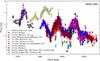 |
Fig. 1 Historical total flux-density light curves of B0605−085 at ten frequencies from 408 MHz to 230 GHz (see text and Table 1). |
2. Total flux-density light curves
2.1. Observations
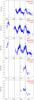 |
Fig. 2 Total radio flux-density light curves of B0605−085 at five frequencies. The solid lines mark the positions of the brightest flares. |
For investigating the long-term radio variability of B0605−085 we used University of Michigan Radio Astronomical Observatory (UMRAO) monitoring data at 4.8 GHz, 8 GHz and 14.5 GHz (Aller et al. 1999) complemented with the archival data from 408 MHz to 230 GHz. Table 1 lists the observed frequency, the time span of the observations, and references. All references in the table refer to the earlier published data. We analyze total flux-density variability of the quasar at ten frequencies obtained at the University of Michigan Radio Astronomical Observatory, Metsähovi Radio Astronomical Observatory, Haystack observatory, Bologna interferometer, Algonquin Radio Observatory, and SEST telescope. The UMRAO data at 4.8 GHz, 8 GHz, and 14.5 GHz since March 2001 are unpublished, whereas data from all other telescopes are archival and have been published earlier.
The historical light curve is shown in Fig. 1 and spans almost 40 years of observations. The longest light curve at an individual frequency covers more than 30 years at 8 GHz (see Table 1). The individual light curves at 4.8, 8, 14.5, 22, and 37 GHz are shown in Fig. 2. The total-flux density variability of B0605−085 shows hints of a periodical pattern. Four maxima have appeared at epochs around 1972.5, 1981.5, 1988.3, and 1995.8 with an almost similar time separation. The last three peaks have a similar brightness at centimeter wavelengths, whereas the first one is around 1 Jy brighter. The data at 22 GHz and 37 GHz are less frequent and cover shorter time ranges of observations, but it is still possible to see that the last peak in 1995–1996 is of a similar shape and reaches the maximum at the same time as at lower frequencies.
The flares at 14.5 GHz show a substructure with the dip in the middle of a flare of about 0.5 Jy, which is ~30% of flare amplitude, suggesting more complex structure of the outburst or possible double-structure of the flares. Figure 3 shows a close-up view of the complex sub-structure of flares at 14.5 GHz. In order to check whether the flares might show the double-peak structure, we fitted the sub-structure of outbursts at 14.5 GHz with the Gaussian functions (dotted lines in Fig. 3). The sum of the Gaussian functions (solid line) follows the light curve fairly well and the possible double peaks have similar separation, they have a time difference of 2.11 years between 1986.43 and 1988.54 sub-flares and 1.92 years between the 1994.45 and 1996.37 sub-flares.
We also searched for archival data at optical wavelengths. However, owing to the close proximity of a very bright foreground star of 9th magnitude, optical observations of this quasar are difficult and there are not enough data for reconstructing the optical light curves.
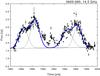 |
Fig. 3 Complex substructure of flares at 14.5 GHz. The dotted lines show the Gaussian functions fitted to the substructure of flares. The solid line is the sum of fitted Gaussian functions. |
2.2. Periodicity analysis
In order to check for possible periodical behavior of flares in the B0605−085 total
flux-density radio light curves we applied the discrete auto-correlation function (DACF)
method (Edelson & Krolik 1988; Hufnagel
& Bregman 1992) and the date-compensated
discrete Fourier transform method (Ferraz-Mello 1981). The discrete auto-correlation function method permits us to study the
level of auto-correlation in unevenly sampled data sets and avoid interpolation or the
addition of artificial data points. The values are combined in pairs
(ai,bj),
for each 0 ≤ i,j ≤ N, where N is the
number of data points. First, the unbinned discrete correlation function is calculated for
each pair 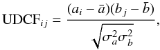 (1)where
 ,
,
 are the mean values of the data series, and
σa,
σb are the corresponding standard
deviations. The discrete correlation function values (DCF) for each time range
Δtij = tj − ti
are calculated as an average of all UDCF values, which time interval falls into the range
τ − Δτ/2 ≤ Δtij ≤ τ + Δτ/2,
where τ is the center of the bin. The higher the value of
Δτ is the better is the accuracy and the worse is the time resolution
of the correlation curve. For the auto-correlation function, the signal is
cross-correlated with itself and a = b,
are the mean values of the data series, and
σa,
σb are the corresponding standard
deviations. The discrete correlation function values (DCF) for each time range
Δtij = tj − ti
are calculated as an average of all UDCF values, which time interval falls into the range
τ − Δτ/2 ≤ Δtij ≤ τ + Δτ/2,
where τ is the center of the bin. The higher the value of
Δτ is the better is the accuracy and the worse is the time resolution
of the correlation curve. For the auto-correlation function, the signal is
cross-correlated with itself and a = b,
 ,
and
σa = σb.
The error of the DACF is calculated as a standard deviation of the DCF value from the
group of unbinned UDCF values
,
and
σa = σb.
The error of the DACF is calculated as a standard deviation of the DCF value from the
group of unbinned UDCF values ![Mathematical equation: \begin{equation} \sigma(\tau) = \frac{1}{M - 1} \left( \sum \left[\mathrm{UDCF}_{ij} - \mathrm{DCF}(\tau) \right] ^2 \right)^{1/2}. \end{equation}](/articles/aa/full_html/2011/02/aa14968-10/aa14968-10-eq27.png) (2)The DACF method
yields different numbers of UDCF per bin, which can affect the final correlation curve. In
order to check the results of the DACF we also applied the Fisher
z-transformed DACF method, which allows us to create data bins with an
equal number of pairs (Alexander 1997).
(2)The DACF method
yields different numbers of UDCF per bin, which can affect the final correlation curve. In
order to check the results of the DACF we also applied the Fisher
z-transformed DACF method, which allows us to create data bins with an
equal number of pairs (Alexander 1997).
The date-compensated discrete fourier transform (DCDFT) method was created to avoid the problem of finiteness of the Fourier transform and allows us to estimate timescales of variability in unevenly sampled data with better precision. The method is based on a power spectrum estimation fitting sinusoids with various trial frequencies to the data set. For a periodic process formed by several waves, the DCDFT method permits us to filter the time series with an already known frequency and to find additional harmonics.
We searched for periods in the light curves at 4.8 GHz, 8 GHz, and 14.5 GHz, which span more than 30 years. We removed a trend before applying a periodicity analysis. The trend was estimated by fitting a linear regression function to the light curve. The auto-correlation method reveals periods of 7.7 ± 0.2 yr at 14.5 GHz, 7.2 ± 0.1 yr at 8 GHz, and 8.0 ± 0.2 yr at 4.8 GHz with high correlation coefficients of 0.84, 0.77, and 0.83 respectively. We estimated the periods by fitting a Gaussian function to the DACF peak. The error bars are calculated as the error bars from the fit. The Fisher z-transformed method for calculating DACF provides the same results. An example of calculated discrete auto-correlation function at 14.5 GHz is shown in Fig. 4 (left). The plot shows a smooth correlation curve with a large amplitude of about 0.8, which is an evidence for a strong period. The date-compensated Fourier transform method also shows a strong periodicity of about eight years. This method indicates a period of 8.4 years with an amplitude of 0.6 Jy at 14.5 GHz, 7.9 years with amplitude of 0.6 Jy at 8 GHz, and 8.5 years with amplitude of 0.3 Jy at 4.8 GHz. In Fig. 4 (right) we plot a periodogram calculated for the 8 GHz data. The dashed line marks a 5% probability to get a periodogram value by chance. The peak corresponding to the detected period is clearly distinguishable from the noise level and has a high amplitude of about 0.6 Jy. The periodogram peak reaches 166.01 at the frequency 0.1268 yr-1, which corresponds to the period of 7.88 years. The probability to get this peak by chance is less than 10-16. The estimated periods are much longer at 4.8 GHz and 14.5 GHz than at 8 GHz, which might be due to the different length of the observations at different frequencies. The light curves at 4.8 GHz and 14.5 GHz span about 23 years (if we do not take into account a few data points in 1970 at 14.5 GHz), whereas the light curve at 8 GHz lasts for 35 years, includes 4 periods and therefore provides a more reliable estimate of the period. The periodicity analysis might show longer periods at 4.8 GHz and 14.5 GHz with the lack of the first peaks in the light curves. The comparison of the obtained sinusoidal signal, where the wavelength and phase are equal to the measured period, with the observed light curves is shown in Figs. 5 (14.5 GHz and 8 GHz) and 6 (4.8 GHz). It is evident from the plots that these sinusoids fairly well follow the observed flux-density variability for all four flares. The main difference is the absence of the last peak in 2003–2006 (expected maximum in 2005.9 at 4.8 GHz, 2002.9 at 8 GHz, and 2004.1 at 14.5 GHz), which is predicted by the periodicity analysis, but is not observed. Both methods give similar results, and one can calculate an average period of 7.9 ± 0.5 years for all three frequencies and for the two methods.
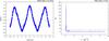 |
Fig. 4 Left: discrete auto-correlation function for 14.5 GHz measurements. Right: results of the date-compensated discrete Fourier transform of the 8 GHz flux-density data. The dashed line marks a 5% probability to get a peak by chance. |
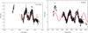 |
Fig. 5 Total flux-density light curves of B0605−085 at 14.5 GHz and 8 GHz. The red line shows sinusoids derived from the date-compensated Fourier transform method with periods of 8.4 and 7.9 years respectively. |
The four main peaks in the total flux-density light curve indicate a periodical behavior of about eight years. If the period is preserved over time, we would expect a powerful outburst in ~2004. However, after the year 2000, the flux-density of B0605−085 stayed at the same flux level of about 1.7 Jy at all five frequencies.
2.3. Frequency-dependent time delays
For a variability caused solely by jet precession we can expect that the flares will appear simultaneously at all frequencies. In order to check whether the peaks at different frequencies reach a maximum at the same time, we calculated frequency-dependent time delays. The Gaussian functions were fitted to the light curves at 4.8 GHz, 8 GHz, 14.5 GHz, 22 GHz, 37 GHz, and 90 GHz, as was described in Pyatunina et al. (2006, 2007). The frequency-dependent time delays were estimated as the time difference between the Gaussian peaks at different frequencies. Owing to insufficient data, it was possible to calculate frequency-dependent time delays only for the outbursts of 1988 and 1995–1996. However, from Fig. 1 it is evident that the 1973 flare appeared almost simultaneously at 8 GHz and 14.5 GHz. We were not able to get reliable fits for the frequencies 22 GHz and 37 GHz due to sparse observations.
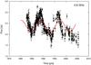 |
Fig. 6 Total flux density light curve of B0605−085 at 4.8 GHz. The red line shows a sinusoid with a period of 8.5 years, derived from the date-compensated Fourier transform method. |
The parameters of the Gaussians fitted to the light curves are shown in Table 2, where frequency, amplitude of a flare, time of the maximum, width of a flare Θ, and time delay are listed. We calculated frequency-dependent time delays with respect to the position of the peak at the highest frequency (22 GHz for the 1995–1996 flare and at 90 GHz for the 1988 flare). It can be clearly seen that the C outburst in 1988 appeared almost simultaneously at all four frequencies with the negligible difference in time between individual frequencies of about 0.08 ± 0.05 years. The 1995–1996 flare D shows similar properties, the light curves at all frequencies have reached the maxima almost simultaneously in about 1995.9, except for 4.8 GHz, which has a delay of 0.43 ± 0.07 years. On the other hand, the data at 4.8 GHz are poorly sampled during the flare rise, which could shift the Gaussian peak. We also calculated frequency-dependent time lags with the cross-correlation function. Table 3 shows the delays between various frequencies for the C and D flares. The delays for the C flare are zero within the error bars. The D flare has shown the large time delay of 0.69 ± 0.05 years between 4.8 GHz and 22.0 GHz, whereas the lags at all other frequencies are much shorter, from 0.08 ± 0.02 to 0.19 ± 0.03 years. These values are consistent with the lags obtained from the Gaussian fitting, especially where we obtained the longer time delay at 4.8 GHz and lower lags at other frequencies. The 1982 flare is poorly sampled, but it is evident from the plot in Fig. 1 that it appeared almost simultaneously at 8 GHz and at the low frequency of 408 MHz. The 1973 flare was observed only at 8 GHz and 14.5 GHz. There are not enough data for this flare to fit Gaussian functions, but it is evident from Fig. 1 that the rising of the flare appears simultaneously at two frequencies. Therefore, we can conclude from the Gaussian fitting and from the visual analysis of the flares that the 1973, 1988, and 1995–1996 outbursts appeared almost simultaneously at different frequencies.
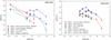 |
Fig. 7 Spectral evolution of B0605−085 during the 1988 flare (left) and 1995–1996 (right). It is evident how the spectral shape changes from steep at the beginning and at the end of the flares to flat during the maxima. |
The bright outbursts appearing simultaneously at all frequencies can be an evidence for a
periodic total flux-density variability caused by the jet precession. We would expect that
if the total flux-density variability is solely due to changes in the Doppler factor, the
peaks of flares should appear at the same time at various frequencies, because the
flux-density Sj is changing like
 , where
α is the spectral index (Lind & Blandford 1985).
, where
α is the spectral index (Lind & Blandford 1985).
B0605−085: parameters of outbursts.
B0605−085: time delays estimated with the cross-correlation method.
2.4. Spectral evolution
In order to check whether all outbursts in the total flux-density light curves have similar spectral properties, we constructed the quasi-simultaneous spectra for all available frequencies. We selected and plotted spectra for various states of variability of B0605−085, such as minimum, rising, maximum, and falling states. Figure 7 shows the spectral evolution observed for the 1988 (left) and 1995–1996 (right) bright outbursts. The 1988 flare starts from a steep spectrum in 1983 and 1984, which then changes its turnover frequency in 1986. During the maximum of the 1988 flare, the spectrum becomes flat and then steepens again during the minimum state after the flare. The 1995–1996 flare shows a similar spectral evolution, with a steep spectrum at the beginning and at the end of the flare and a flat spectral shape during the maximum (Fig. 7).
The light curve of B0605−085 consists of four periodical flares in 1973, 1981, 1988, and 1995–1996. The last two flares have a similar spectral evolution and a similar brightness. The observations during the 1973 flare are much sparser, but a historical radio light curve shows that the fluxes at 8 GHz and 14.5 GHz are similar, which indicates a flat spectrum. However, note that the second 1981 flare shows a completely different spectral behavior. One can see from the historical light curve (see Fig. 1) that the spectrum of this flare is steep, because the brightness at 408 MHz significantly exceeds the brightness at centimeter wavelengths. Therefore, we can conclude that although the periodical flares look almost similar in brightness, they reveal different spectral properties.
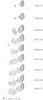 |
Fig. 8 Contour images of B0605−085 and overlapped on them circular Gaussian components to model the observed visibilities (see Table 5). The distance between images on the plot is proportional to the time passed. |
3. Kinematics of B0605−085
3.1. Observations
For an investigation of the B0605−085 jet kinematics we analyzed nine epochs of VLBA observations at 15 GHz from the MOJAVE and 2cm survey programs (http://www.physics.purdue.edu/astro/MOJAVE/). The observations were performed between 1995.6 and 2005.7. The data were fringe-fitted and calibrated before by the MOJAVE collaboration (Lister & Homan 2005; Kellermann et al. 2004). Lister et al. (2009) and Homan et al. (2009) discussed jet components movement and acceleration in this source in a framework of statistical studies of the sample of 135 active galaxies. In this paper we aim to study the motion of the B0605−085 jet components in more detail, avoiding pre-established initial models during the model-fitting process.
We performed map cleaning and model fitting of circular Gaussian components with the
Difmap package (Shepherd 1997).
We used a uniform weighting scheme for map cleaning. Circular components were chosen in
order to avoid extremely elongated components and to facilitate the comparison of the
features and their identification. In order to find the optimum set of components and
parameters, we fitted every data set starting from a point-like model, adding a Gaussian
component after each run of model fitting. The position errors of core separation and
position angle were estimated as  and
Δθ = arctan(Δr/r), where
σrms is the residual noise of the map after the subtraction
of the model, d is the full-width-at-half maximum (FWHM)
of the component and Speak is the peak flux density (Fomalont
1999). However, this formula tends to
underestimate the error if the peak flux density is very high or the width of a component
is small. Therefore, uncertainties have also been estimated by comparison of different
model fits (±1 component) obtained for the same set of data. This permits us to check
for possible parameter variations of individual jet components during model-fitting. The
final position error was calculated as a maximum value of error bars obtained by two
methods.
and
Δθ = arctan(Δr/r), where
σrms is the residual noise of the map after the subtraction
of the model, d is the full-width-at-half maximum (FWHM)
of the component and Speak is the peak flux density (Fomalont
1999). However, this formula tends to
underestimate the error if the peak flux density is very high or the width of a component
is small. Therefore, uncertainties have also been estimated by comparison of different
model fits (±1 component) obtained for the same set of data. This permits us to check
for possible parameter variations of individual jet components during model-fitting. The
final position error was calculated as a maximum value of error bars obtained by two
methods.
The final hybrid maps with fitted Gaussian components are shown in Fig. 8. We list all parameters of jet components, such as the core separation, the position angle, the flux-density, the size, and identification for all epochs in Table 5.
3.2. The component identification
The component identification was performed in a way that the core separation, the position angle, and the flux of jet features change smoothly between adjacent epochs. In order to obtain the best identification, the jet components were labeled in different ways, and the identification which gave the smoothest changes in all parameters of jet features, such as mean flux and position, was chosen as the final set. The core separations and the flux densities of each individual jet component are shown in Fig. 9, left and right respectively. Individual jet features are marked by different colors. Jet feature C1 appears quasi-stationary at an average core separation of 3.7 mas with a flux density of about 0.1 Jy at all epochs. It is marked with a dotted line in the plot. This quasi-stationary feature is well-detected in the first four epochs, but after 2002 it is blended with the outward moving jet component d2, which was ejected in ~1998. This feature may be explained with a co-existence of a stationary component and jet features moving outward. Four outward moving jet components (da, d0, d1, d2, and d3) were ejected during the time of the observations, whereas the components d6 and d7 are located at a range of core separations between 6 and 8 mas, showing slow outward movement and have probably been ejected earlier. The jet components which were ejected at the time of observations are at a level of 0.3–0.4 Jy after ejection, and then their flux-density fades down to 0.1 Jy level or less.
Summary of the features’ speeds based on the model-fits.
3.3. Component ejections
We found seven jet components moving outward with apparent speeds from 0.12 to 0.66 mas/yr, which corresponds to speeds of 5.6 c–31 c (see Table 4). The d3 component has been ejected in 1996.9 during the 1995–1996 outburst, after the flare had reached its peak. All other components ejected after the d3 feature, such as d1, d0, and da, show decreasing speeds for almost each successive component. The jet component d3 has a speed of 0.66 ± 0.01 mas/yr, the next feature d2 has speed of 0.57 ± 0.01 mas/yr, d1 has 0.44 ± 0.01 mas/yr, d0 has 0.46 ± 0.02 mas/yr, and the last component da has 0.12 ± 0.03 mas/yr. A few faint Gaussian components could not be identified between different epochs (marked by black dots in Fig. 9). These components reveal flux-densities on the order of 0.05 Jy, and can either be blobs which were ejected before 1995 and cannot be traced because of lack of data, or can be possibly trailing components (e.g., Agudo et al. 2001; Kadler et al. 2008).
The Doppler factor of a jet depends on the Lorentz factor γ, the angle
between the jet flow direction and the line of sight φ, and the speed of
a jet component in the source frame β:
 (3)With the velocity of the
jet component with the highest speed one can calculate the maximal viewing angle
(3)With the velocity of the
jet component with the highest speed one can calculate the maximal viewing angle
 (4)and a lower limit for
the Lorentz factor
(4)and a lower limit for
the Lorentz factor  (5)assuming that the highest
apparent speed detected defines the lowest possible Lorentz factor of the jet (e.g.,
Pearson & Zensus 1986). The fastest jet
component of B0605−085 is d3, which has a speed of
31c. The corresponding Lorentz factor is
γmin = 31 and the upper limit for the viewing angle is
φmax = 3.7°, which gives us an estimation for the Doppler
factor δmin = 12.4. For smaller viewing angles
(φ → 0) the Doppler factors approach a value of 62, which yields a
range of the Doppler factors δ = 12.4 to 62 at viewing angles between
3.7° and 0°.
(5)assuming that the highest
apparent speed detected defines the lowest possible Lorentz factor of the jet (e.g.,
Pearson & Zensus 1986). The fastest jet
component of B0605−085 is d3, which has a speed of
31c. The corresponding Lorentz factor is
γmin = 31 and the upper limit for the viewing angle is
φmax = 3.7°, which gives us an estimation for the Doppler
factor δmin = 12.4. For smaller viewing angles
(φ → 0) the Doppler factors approach a value of 62, which yields a
range of the Doppler factors δ = 12.4 to 62 at viewing angles between
3.7° and 0°.
The instantaneous speeds of the jet components have been calculated as the core separation difference between two subsequent positions of a jet component divided by the time elapsed between these two observations. The jet components d1, d3, and C1 show significant changes of instantaneous speeds, which indicates that they experience acceleration and deceleration along the jet (see Fig. 10 for the jet component d1). Figure 11 shows the averaged instantaneous speeds of all jet components in the 1-mas core separation bins. We calculated instantaneous speeds between each data point for each jet component and then averaged all the instantaneous speeds for data points located within a certain bin of core separation. The average instantaneous speeds of all jet components accelerate at about 0.1 mas, 3 mas, 6 mas, and 9 mas distance from the core and decelerate at 2 mas, 5 mas, and 7 mas, which indicates a characteristic scale of 3 mas for acceleration/deceleration of the jet components. The helical pattern of the speeds might be due to a helical pattern of the jet and multiple bends on the way of the jet components. Note that the characteristic spatial scale of 3 mas corresponds to a timescale of about 7.7 years (using the average speed of the jet components 0.39 mas/yr), which is similar to the periodic timescale of the variability in the total flux-density.
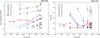 |
Fig. 9 Left: core separation as function of time at 15 GHz. Individual jet components are marked by different colors. Right: time variability of jet components’ flux density. |
3.4. Quasi-stationary component C1
The quasi-stationary component C1 is a well-defined feature from 1995 to 2001 (see Fig. 9). However, after 2002 it is most probably blended with the moving jet component d2. Earlier than 2002, when the quasi-stationary component is clearly identified, there were no moving jet components. That might explain why the component C1 was blended only after 2002. As the newly ejected jet feature approach the position of component C1, it becomes harder to distinguish them and it is more likely that we see blending of two components. Blending and dragging of stationary jet components by moving components was predicted from the magneto-hydrodynamical simulations by Gomez et al. (1997) and Aloy et al. (2003) and was observed in a large number of sources (e.g., 3C 279 Wehrle et al. 2001; S5 1803+784 Britzen et al. 2005; 0735+178 Gabuzda et al. 1994).
The quasi-stationarity of jet component C1 can be due to various physical mechanisms. It can be caused by jet bending or by stationary conical shockwaves appearing because of an interaction with the ambient medium (e.g., Alberdi 2000; Gomez et al. 1997). If the stationary feature in the jet is caused by jet bending towards us, then we can expect a significant flux-density increase in other jet components in the area close to the position of the stationary feature due to relativistic boosting. When we plot the flux-density versus core separation for all detected Gaussian components (excluding the core) in Fig. 12 we see that at core separations between 2.5 and 6.2 mas there is a significant increase in flux-density values. This increase is independent of the component identification and might be explained by a jet-bending in the area around 4 mas. Moreover, this jet-bending can explain the existence of the quasi-stationary jet feature C1, which is located at a similar core separation of about 3.7 mas.
High-resolution VLBI maps of the quasar B0605−085 were discussed in several papers (e.g., Padrielli et al. 1986, 1991; Bondi et al. 1996b). A stationary jet component observed at 2 and 5 GHz in 1997 at a core separation similar to C1 was reported before by Fey & Charlot (2000). They found the jet components at a core separation of 3.0 mas and PA = 100°, which is similar to the position of the C1 component. This is additional evidence for the stationarity of the jet component C1.
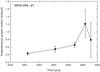 |
Fig. 10 Instantaneous speeds of the jet component d1, which experiences significant acceleration when moving along the jet. |
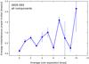 |
Fig. 11 Instantaneous speeds of all jet components of B0605−085 averaged in 1 mas core separation bins. |
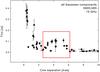 |
Fig. 12 Flux-density of all Gaussian components found in the jet of B0605−085 at 15 GHz. The core was excluded from the plot to show smaller range of flux densities. It is evident that all components become significantly brighter when they are at the range of the core separations from 2.5 to 6.2 mas, which can be explained by the jet-bending. |
The quasi-stationary jet component C1 is located at an average core separation of 3.7 mas. However, the position of this component changes with time from 2.95 to 4.32 mas. The position angle and the flux-density of C1 are also variable. Figure 13 shows these changes over time in core separation, position angle, and flux-density. The position angle and the flux-density of the component are anti-correlated. The position angle reaches its maximum value of 125 degrees in 2001, when the flux is at the minimum value of 0.013 ± 0.002 Jy. There is also a possible connection between the core separation and the flux-density of the component C1 – both of them have minima in about 2001–2003 and then experience a rise with a maximum in 2005. In rectangular coordinates, the trajectory of the quasi-stationary jet component C1 follows a clear helical path. Figure 14 shows a trajectory of C1 in the plane of the sky. It is evident from the plot that the quasi-stationary component follows a spiral trajectory. Moreover, the characteristic timescale of a helix turn is about 8 years. This timescale is very close to the value of the period of the total flux-density variability discussed earlier. This might be evidence for a possible connection between the helical movement of C1 and the total flux-density periodicity. The jet might precess and therefore we will see periodic flares in the light curves due to the variability of the Doppler boosting as well as changes of position of a bend in the jet.
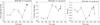 |
Fig. 13 Time evolution of core separation (left), position angle (middle) and flux-density (right) of the quasi-stationary component C1. |
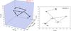 |
Fig. 14 Trajectory of the quasi-stationary component C1 in rectangular coordinates in three-dimensional space with the third axis showing the time (left) and in two dimensions (right). The trajectory of the component seems to follow a helical path. |
3.5. Comparison of trajectories
We plot the position angles of all features da–d7, including the quasi-stationary component C1, versus the core separation in Fig. 15. The trajectories of the components d1, d2, d6, d7, and C1 follow significantly curved trajectories, whereas the trajectories of the components d0 and d3 follow a linear path. This can be an evidence for a possible co-existence of two types of jet component trajectories, similar to the source 3C 345 (Klare et al. 2005). The spread of position angles of all components is changing along the jet. In the inner part, within the first 1 mas, the position angles are in the range of 123–150 degrees, in the middle part of the jet between 1–5 mas, the position angles range from 110° to 125°, whereas in the outer part from 5 mas to 10 mas, they range from 95° to 115°.
Model-fit results for B0605−085 at 15 GHz.
4. Precession model
The probable periodical variability of the radio total flux-densities of B0605−085 and
the helical motion of the quasi-stationary jet component C1 can be
explained by jet precession. We used the precession model described in Abraham &
Carrara (1998) and Caproni & Abraham (2004) for fitting the helical path of the jet component
C1. In this model, the rectangular coordinates of a precession cone in
the source frame are changing with time t′ due to precession: ![Mathematical equation: \begin{eqnarray} \label{eq:x_t}X(t') &=& [\cos \Omega \sin \phi_{0} + \sin \Omega \cos \phi_{0} \sin \omega t'] \cos \eta_{0} \nonumber\\ &&-\sin \Omega \cos \omega t' \sin \eta_{0}, \\ \label{eq:y_t}Y(t') &=& [\cos \Omega \sin \phi_{0} + \sin \Omega \cos \phi_{0} \sin \omega t'] \sin \eta_{0} \nonumber\\ && + \sin \Omega \cos \omega t' \cos \eta_{0}, \end{eqnarray}](/articles/aa/full_html/2011/02/aa14968-10/aa14968-10-eq328.png) where
Ω is the semi-aperture angle of the precession cone, φ0 is the
angle between the precession cone axis and the line of sight and is actually the average
viewing angle of the source, and η0 is the projected angle of
the cone axis onto the plane of the sky (see Fig. 16).
The angular velocity of the precession is ω = 1/P, where
P is the period. We take a P value of 7.9-year
(timescale found in the total flux-density radio light curves and in the helical movement of
C1). The time in the source frame (t′) and the frame of
the observer (t) are related by the Doppler factor δ as
where
Ω is the semi-aperture angle of the precession cone, φ0 is the
angle between the precession cone axis and the line of sight and is actually the average
viewing angle of the source, and η0 is the projected angle of
the cone axis onto the plane of the sky (see Fig. 16).
The angular velocity of the precession is ω = 1/P, where
P is the period. We take a P value of 7.9-year
(timescale found in the total flux-density radio light curves and in the helical movement of
C1). The time in the source frame (t′) and the frame of
the observer (t) are related by the Doppler factor δ as
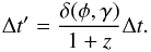 (8)However, the only
time-dependent term in Eqs. (6) and (7) is ωt, which does not depend
on this time corrections because ω ~ 1/t.
Therefore, we can fit the trajectory in the rectangular coordinate
X(t) of the quasi-stationary jet component
C1, using Eq. (6). We
assume that the motion of C1 reflects the movement of the jet. The
non-linear least-squares method was used for the precession model fitting. The angular
velocity of the precession ω and the redshift of the source
z are known and we fix them during the fit, whereas the aperture angle of
the precessing cone Ω, φ0, and η0
are used as free parameters. The results of the fit are shown in Fig. 17 (left) and the parameters of the precession model for the parsec jet
of B0605−085 are listed in Table 6. The precession
model well fits the trajectory of the quasi-stationary jet component C1.
The same parameters were used to describe the motion of C1 in declination.
The model for the declination is shown in Fig. 17
(right).
(8)However, the only
time-dependent term in Eqs. (6) and (7) is ωt, which does not depend
on this time corrections because ω ~ 1/t.
Therefore, we can fit the trajectory in the rectangular coordinate
X(t) of the quasi-stationary jet component
C1, using Eq. (6). We
assume that the motion of C1 reflects the movement of the jet. The
non-linear least-squares method was used for the precession model fitting. The angular
velocity of the precession ω and the redshift of the source
z are known and we fix them during the fit, whereas the aperture angle of
the precessing cone Ω, φ0, and η0
are used as free parameters. The results of the fit are shown in Fig. 17 (left) and the parameters of the precession model for the parsec jet
of B0605−085 are listed in Table 6. The precession
model well fits the trajectory of the quasi-stationary jet component C1.
The same parameters were used to describe the motion of C1 in declination.
The model for the declination is shown in Fig. 17
(right).
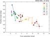 |
Fig. 15 Position angle changes of the jet components da–d7, including the quasi-stationary component C1 at 15 GHz. |
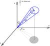 |
Fig. 16 Jet precession geometry. The line of sight is parallel to the z-axis. |
We found another set of parameters Ω = 92.2°, φ0 = 69.8°,
η0 = 12.9° as one of the possible solutions. However, the
viewing angle is very large. Using the equation 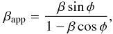 (9)and taking average
value of apparent speeds βapp, aver = 16.5c,
we can calculate the speed in the source frame β = 2.49c,
which is higher then the speed of light. A precession cone aperture angle Ω = 92.2° is also
unlikely. Therefore, this set of parameters is not plausible. The solution in Table 6 is the only physically feasible, because the complete
parameter space was covered during the fitting procedure.
(9)and taking average
value of apparent speeds βapp, aver = 16.5c,
we can calculate the speed in the source frame β = 2.49c,
which is higher then the speed of light. A precession cone aperture angle Ω = 92.2° is also
unlikely. Therefore, this set of parameters is not plausible. The solution in Table 6 is the only physically feasible, because the complete
parameter space was covered during the fitting procedure.
5. Discussion
Assuming that the helical motion of the quasi-stationary jet component C1
is caused solely by jet precession (with a period of eight years), we were able to determine
the geometrical parameters of the jet precession, such as the aperture angle of a precession
cone, the viewing angle, and the projection angle. The fitted viewing angle
φ0 = 2.6° ± 2.2° agrees well with the upper limit for the
viewing angle deduced from the apparent speeds of the jet components
φmax = 3.7°. It is also similar to the viewing angle
φvar = 5° derived from the radio total flux-density
variability by Hovatta et al. (2008). The jet
precession will also cause the periodical variability of the radio total flux-density light
curves with the same period of eight years, owing to periodical changes of the Doppler
factor. The flux density Sj is changing with
the Doppler factor due to the jet precession , where
α is the spectral index (Lind & Blandford 1985). From this equation we can expect that the flares due to the jet
precession will appear simultaneously at different frequencies, which is actually observed
for the major outbursts in 1973, 1988, and 1995–1996. Therefore, the jet precession is
probably responsible for the total flux-density variability, periodicity in the outbursts,
and the helical motion of the quasi-stationary jet component C1.
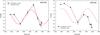 |
Fig. 17 Sky trajectory of the quasi-stationary component C1 in right ascension (left) and declination (right). The solid line shows the fit of the precession model. The precession model well fits the trajectory of a quasi-stationary jet component C1. |
Some questions remain. It is still not known why the four major outbursts in the total flux-density light curve, which repeat periodically with an 8-year period, have different spectral properties. Longer monitoring of this quasar at several frequencies is necessary in order to understand the spectral properties of the flares.
The precession of B0605−085 jet can be caused by several physical mechanisms. Jet instabilities, a secondary black hole rotating around the primary black hole, and accretion disk instabilities might be responsible for the observed changes of jet direction (e.g., Camenzind & Krockenberger 1992; Hardee & Norman 1988; Lobanov & Roland 2005). At the moment it is impossible to claim exactly which mechanism produces the observed jet precession. Note though that the possible double-peak structure of the flares at 14.5 GHz in B0605−085 is similar to the double-peak flares of OJ 287 that are observed in optical light curves which were explained by the orbiting secondary black hole. At the moment we cannot say whether there is a secondary black hole in the center of a hosting galaxy in B0605−085, and more observations and theoretical modeling are needed.
The next total flux-density flare of the source might appear in 2012 if the 8-year period is preserved over time. The 8-year period in the flux-density variability has predicted the next powerful outburst to appear in ~2004. However, the flare was of a very low flux level, which might be due to a long-term trend in the flux-density variability. Recent observations of B0605−085 have shown a rise in fluxes, which might suggest a probable peak close to 2012, taking into account the duration of the outbursts in this source. This will mean that the 8-year period interferes with long-term changes of the flux-densities. More radio total flux-density and VLBI observations are needed in order to check this prediction.
6. Summary
The results of our analysis of the jet kinematics in B0605−085 are:
-
We find strong evidence for a period on the order of eight years (7.9 ± 0.5 years when averaged over frequencies) in the total flux-density light curves at 4.8 GHz, 8 GHz and 14.5 GHz, which was observed for four cycles.
-
The measurement of frequency-dependent time delays for the brightest outbursts in 1988, and 1995–1996 and the visual analysis for the 1973 flare shows that these flares appeared almost simultaneously at all frequencies.
-
The spectral analysis of the flares shows that the main flares in 1973, 1988, 1995–1996 have a flat spectrum, whereas the flare in 1981 has a steep spectrum, which suggests that the four cycles of the 8-year period have different spectral properties.
-
The average instantaneous speeds of the jet components reveal a helical pattern along the jet axis with a characteristic scale of 3 mas. This scale corresponds to a timescale of about 7.7 years, which is similar to the periodicity timescale found in the total flux-densities.
-
The quasi-stationary jet component C1 follows a helical path with a period of eight years. This timescale coincides with the period found in the total flux-density light curves.
-
We found evidence that the jet components of B0605−085 follow two different types of trajectories. Some components move along straight lines, whereas other components follow significantly curved paths.
-
The fit of the precession model to the trajectory of the quasi-stationary jet component C1 has shown that it can be explained by changes of the jet direction with a precession period of P = 8 yrs (in the observers frame), an aperture angle of the precession cone Ω = 23.9° ± 1.9°, a viewing angle φ0 = 2.6° ± 2.2°, and a projection angle η0 = 33.6° ± 6.5°.
Acknowledgments
This research has made use of data from the MOJAVE database that is maintained by the MOJAVE team (Lister et al. 2009, AJ, 137, 3718). N. A. Kudryavtseva and M. Karouzos were supported for this research through a stipend from the International Max Planck Research School (IMPRS) for Astronomy and Astrophysics. We would like to thank Christian Fromm for fruitful discussions and help with the picture. This research has made use of data from the University of Michigan Radio Astronomy Observatory, which is supported by the National Science Foundation and by funds from the University of Michigan. The Alonquin Radio Observatory is operated by the National Research Council of Canada as a national radio astronomy facility. The operation of the Haystack Observatory is supported by the grant from the National Science Foundation. The National Radio Astronomy Observatory is a facility of the National Science Foundation operated under cooperative agreement by Associated Universities, Inc. This publication has emanated from research conducted with the financial support of Science Foundation Ireland. This research has made use of the SIMBAD database, operated at CDS, Strasbourg, France. We thank the anonymous referee for a careful reading of the manuscript and useful comments and suggestions that have improved this paper.
References
- Abraham, Z., & Carrara, E. A. 1998, ApJ, 496, 172 [NASA ADS] [CrossRef] [Google Scholar]
- Agudo, I., Gómez, J.-L., Martí, J.-M., et al. 2001, ApJ, 549, 183 [Google Scholar]
- Alexander, T. 1997, in Astronomical Time Series, ed. D. Maoz, A. Sternberg, & E. M. Leibowitz (Dordrecht: Kluwer), 163 [Google Scholar]
- Alberdi, A., Gómez, J. L., Marcaide, J. M., Marscher, A. P., & Pérez-Torres, M. A. 2000, A&A, 361, 529 [NASA ADS] [Google Scholar]
- Aller, H. D., Aller, M. F., Latimer, G. E., & Hodge, P. E. 1985, ApJS, 59, 513 [NASA ADS] [CrossRef] [Google Scholar]
- Aller, M. F., Aller, H. D., Hughes, P. A., & Latimer, G. E. 1999, ApJ, 512, 601 [NASA ADS] [CrossRef] [Google Scholar]
- Aller, M. F., Aller, H. D., & Hughes, P. A. 2003, ApJ, 586, 33 [NASA ADS] [CrossRef] [Google Scholar]
- Aloy, M.Á., Martí, J.-M., Gómez, J.-L., et al. 2003, ApJ, 585, 109 [Google Scholar]
- Andrew, B. H., MacLeod, J. M., Harvey, G. A., & Medd, W. J. 1978, AJ, 83, 863 [NASA ADS] [CrossRef] [Google Scholar]
- Bach, U., Villata, M., Raiteri, C. M., et al. 2006, A&A, 456, 105 [NASA ADS] [CrossRef] [EDP Sciences] [Google Scholar]
- Bondi, M., Padrielli, L., Fanti, R., et al. 1996a, A&AS, 120, 89 [Google Scholar]
- Bondi, M., Padrielli, L., Fanti, R., et al. 1996b, A&A, 308, 415 [NASA ADS] [Google Scholar]
- Britzen, S., Witzel, A., Krichbaum, T. P., et al. 2005, MNRAS, 362, 966 [NASA ADS] [CrossRef] [Google Scholar]
- Britzen, S., Kudryavtseva, N. A., Witzel, A., et al. 2010, A&A, 511, A57 [NASA ADS] [CrossRef] [EDP Sciences] [Google Scholar]
- Camenzind, M., & Krockenberger, M. 1992, A&A, 255, 59 [NASA ADS] [Google Scholar]
- Caproni, A., & Abraham, Z. 2004, MNRAS, 349, 1218 [Google Scholar]
- Ciaramella, A., Bongardo, C., Aller, H. D., et al. 2004, A&A, 419, 485 [NASA ADS] [CrossRef] [EDP Sciences] [Google Scholar]
- Cooper, N. J., Lister, M. L., & Kochanczyk, M. D. 2007, ApJS, 171, 376 [NASA ADS] [CrossRef] [Google Scholar]
- Dent, W. A., & Kapitzky, J. E. 1976, AJ, 81, 1053 [NASA ADS] [CrossRef] [Google Scholar]
- Dent, W. A., Kapitzky, J. E., & Kojoian, G. 1974, AJ, 79, 1232 [NASA ADS] [CrossRef] [Google Scholar]
- Edelson, R. A., & Krolik, J. H. 1988, ApJ, 333, 646 [NASA ADS] [CrossRef] [Google Scholar]
- Ferraz-Mello, S. 1981, AJ, 86, 619 [NASA ADS] [CrossRef] [Google Scholar]
- Fey, A. L., & Charlot, P. 2000, ApJS, 128, 17 [NASA ADS] [CrossRef] [Google Scholar]
- Fomalont, E. B. 1999, in Synthesis Imaging in Radio Astronomy II, ed. G. B. Taylor, C. L. Carilli, & R. A. Perley (San Francisco: ASP), ASP Conf. Ser., 180, 301 [Google Scholar]
- Gabuzda, D. C., Wardle, J. F. C., Roberts, D. H., Aller, M. F., & Aller, H. D. 1994, ApJ, 435, 128 [NASA ADS] [CrossRef] [Google Scholar]
- Gómez, J. L., Martí, J. M. A., Marscher, A. P., Ibáñez, J. M. A., & Alberdi, A. 1997, ApJ, 482, 33 [Google Scholar]
- Hardee, P. E., & Norman, M. L. 1988, ApJ, 334, 70 [NASA ADS] [CrossRef] [Google Scholar]
- Homan, D. C., Kadler, M., Kellermann, K. I., et al. 2009, ApJ, 706, 1253 [NASA ADS] [CrossRef] [Google Scholar]
- Honma, F., Kato, S., & Matsumoto, R. 1991, PASJ, 43, 147 [NASA ADS] [Google Scholar]
- Hovatta, T., Valtaoja, E., Tornikoski, M., & Lähteenmäki, A. 2009, A&A, 494, 527 [NASA ADS] [CrossRef] [EDP Sciences] [Google Scholar]
- Hufnagel, B. R., & Bregman, J. N. 1992, ApJ, 386, 473 [NASA ADS] [CrossRef] [Google Scholar]
- Kadler, M., Hughes, P. A., Ros, E., Aller, M. F., & Aller, H. D. 2006, A&A, 456, 1 [Google Scholar]
- Kadler, M., Ros, E., Perucho, M., et al. 2008, ApJ, 680, 867 [NASA ADS] [CrossRef] [Google Scholar]
- Kellermann, K. I., Lister, M. L., Homan, D. C., et al. 2004, ApJ, 609, 539 [NASA ADS] [CrossRef] [Google Scholar]
- Kelly, B. C., Hughes, P. A., Aller, H. D., & Aller, M. F. 2003, ApJ, 591, 695 [NASA ADS] [CrossRef] [Google Scholar]
- Kidger, M. R. 2000, AJ, 119, 2053 [NASA ADS] [CrossRef] [Google Scholar]
- Klare, J., Zensus, J. A., Lobanov, A. P., et al. 2005, in Future Directions in High Resolution Astronomy: The 10th Anniversary of the VLBA, ed. J. Romney, & M. Reid., ASP Conf. Ser., 340, 40 [Google Scholar]
- Kudryavtseva, N. A., & Pyatunina, T. B. 2006, ARep, 50, 1 [NASA ADS] [Google Scholar]
- Lehto, H. J., & Valtonen, Mauri J. 1996, ApJ, 460, 207 [NASA ADS] [CrossRef] [Google Scholar]
- Lind, K. R., & Blandford, R. D. 1985, ApJ, 295, 358 [NASA ADS] [CrossRef] [Google Scholar]
- Lister, M. L., & Homan, D. C. 2005, AJ, 130, 1389 [NASA ADS] [CrossRef] [Google Scholar]
- Lister, M. L., Cohen, M. H., Homan, D. C., et al. 2009, AJ, 138, 1874 [NASA ADS] [CrossRef] [Google Scholar]
- Lobanov, A. P., & Roland, J. 2005, A&A, 431, 831 [NASA ADS] [CrossRef] [EDP Sciences] [Google Scholar]
- Medd, W. J., Andrew, B. H., Harvey, G. A., & Locke, J. L. 1972, MmRAS, 77, 109 [Google Scholar]
- Ostorero, L., Villata, M., & Raiteri, C. M. 2004, A&A, 419, 913 [NASA ADS] [CrossRef] [EDP Sciences] [Google Scholar]
- Padrielli, L., Romney, J. D., Bartel, N., et al. 1986, A&A, 165, 53 [NASA ADS] [Google Scholar]
- Padrielli, L., Eastman, W., Gregorini, L., Mantovani, F., & Spangler, S. 1991, A&A, 249, 351 [NASA ADS] [Google Scholar]
- Pearson, T. J., & Zensus, J. A. 1987, in Superluminal Radio Sources, ed. T. J. Pearson, & J. A. Zensus (Cambridge Univ. Press), 11 [Google Scholar]
- Pyatunina, T. B., Kudryavtseva, N. A., Gabuzda, D. C., et al. 2006, MNRAS, 373, 1470 [NASA ADS] [CrossRef] [Google Scholar]
- Pyatunina, T. B., Kudryavtseva, N. A., Gabuzda, D. C., et al. 2007, MNRAS, 381, 797 [NASA ADS] [CrossRef] [Google Scholar]
- Qian, Shan-Jie, Kudryavtseva, N. A., Britzen, S., et al. 2007, ChJAA, 7, 364 [Google Scholar]
- Raiteri, C. M., Villata, M., Aller, H. D., et al. 2001, A&A, 377, 396 [NASA ADS] [CrossRef] [EDP Sciences] [Google Scholar]
- Reuter, H.-P., Kramer, C., Sievers, A., et al. 1997, A&AS, 122, 271 [Google Scholar]
- Rieger, F. M., & Mannheim, K. 2000, A&A, 359, 948 [NASA ADS] [Google Scholar]
- Sambruna, R. M., Gambill, J. K., Maraschi, L., et al. 2004, ApJ, 608, 698 [NASA ADS] [CrossRef] [Google Scholar]
- Scott, W. K., Fomalont, E. B., Horiuchi, S., et al. 2004, ApJS, 155, 33 [Google Scholar]
- Shepherd, M. C., 1997, in Astronomical Data Analysis Software and Systems VI, ed. G. Hunt, & H. E. Payne, ASP Conf. Ser., 125, 77 [Google Scholar]
- Steppe, H., Salter, C. J., Chini, R., et al. 1988, A&AS, 75, 317 [NASA ADS] [Google Scholar]
- Steppe, H., Liechti, S., Mauersberger, R., et al. 1992, A&AS, 96, 441 [NASA ADS] [Google Scholar]
- Stickel, M., Kühr, H., & Fried, J. W. 1993, A&AS, 97, 483 [NASA ADS] [Google Scholar]
- Stirling, A. M., Cawthorne, T. V., Stevens, J. A., et al. 2003, MNRAS, 341, 405 [NASA ADS] [CrossRef] [Google Scholar]
- Teräsranta, H., Tornikoski, M., Mujunen, A., et al. 1998, A&AS, 132, 305 [NASA ADS] [CrossRef] [EDP Sciences] [Google Scholar]
- Tornikoski, M., Valtaoja, E., Teräsranta, H., et al. 1996, A&AS, 116, 157 [NASA ADS] [Google Scholar]
- Valtaoja, E., Teräsranta, H., Tornikoski, M., et al. 2000, ApJ, 531, 744 [NASA ADS] [CrossRef] [Google Scholar]
- Villata, M., & Raiteri, C. M. 1999, A&A, 347, 30 [NASA ADS] [Google Scholar]
- Villata, M., Raiteri, C. M., Aller, H. D., et al. 2004, A&A, 424, 497 [NASA ADS] [CrossRef] [EDP Sciences] [Google Scholar]
- Villata, M., Raiteri, C. M., Larionov, V. M., et al. 2009, A&A, 501, 455 [NASA ADS] [CrossRef] [EDP Sciences] [Google Scholar]
- Wehrle, A. E., Piner, B. G., Unwin, S. C., et al. 2001, ApJS, 133, 297 [NASA ADS] [CrossRef] [Google Scholar]
All Tables
All Figures
|
Fig. 1 Historical total flux-density light curves of B0605−085 at ten frequencies from 408 MHz to 230 GHz (see text and Table 1). |
| In the text | |
|
Fig. 2 Total radio flux-density light curves of B0605−085 at five frequencies. The solid lines mark the positions of the brightest flares. |
| In the text | |
|
Fig. 3 Complex substructure of flares at 14.5 GHz. The dotted lines show the Gaussian functions fitted to the substructure of flares. The solid line is the sum of fitted Gaussian functions. |
| In the text | |
|
Fig. 4 Left: discrete auto-correlation function for 14.5 GHz measurements. Right: results of the date-compensated discrete Fourier transform of the 8 GHz flux-density data. The dashed line marks a 5% probability to get a peak by chance. |
| In the text | |
|
Fig. 5 Total flux-density light curves of B0605−085 at 14.5 GHz and 8 GHz. The red line shows sinusoids derived from the date-compensated Fourier transform method with periods of 8.4 and 7.9 years respectively. |
| In the text | |
|
Fig. 6 Total flux density light curve of B0605−085 at 4.8 GHz. The red line shows a sinusoid with a period of 8.5 years, derived from the date-compensated Fourier transform method. |
| In the text | |
|
Fig. 7 Spectral evolution of B0605−085 during the 1988 flare (left) and 1995–1996 (right). It is evident how the spectral shape changes from steep at the beginning and at the end of the flares to flat during the maxima. |
| In the text | |
|
Fig. 8 Contour images of B0605−085 and overlapped on them circular Gaussian components to model the observed visibilities (see Table 5). The distance between images on the plot is proportional to the time passed. |
| In the text | |
|
Fig. 9 Left: core separation as function of time at 15 GHz. Individual jet components are marked by different colors. Right: time variability of jet components’ flux density. |
| In the text | |
|
Fig. 10 Instantaneous speeds of the jet component d1, which experiences significant acceleration when moving along the jet. |
| In the text | |
|
Fig. 11 Instantaneous speeds of all jet components of B0605−085 averaged in 1 mas core separation bins. |
| In the text | |
|
Fig. 12 Flux-density of all Gaussian components found in the jet of B0605−085 at 15 GHz. The core was excluded from the plot to show smaller range of flux densities. It is evident that all components become significantly brighter when they are at the range of the core separations from 2.5 to 6.2 mas, which can be explained by the jet-bending. |
| In the text | |
|
Fig. 13 Time evolution of core separation (left), position angle (middle) and flux-density (right) of the quasi-stationary component C1. |
| In the text | |
|
Fig. 14 Trajectory of the quasi-stationary component C1 in rectangular coordinates in three-dimensional space with the third axis showing the time (left) and in two dimensions (right). The trajectory of the component seems to follow a helical path. |
| In the text | |
|
Fig. 15 Position angle changes of the jet components da–d7, including the quasi-stationary component C1 at 15 GHz. |
| In the text | |
|
Fig. 16 Jet precession geometry. The line of sight is parallel to the z-axis. |
| In the text | |
|
Fig. 17 Sky trajectory of the quasi-stationary component C1 in right ascension (left) and declination (right). The solid line shows the fit of the precession model. The precession model well fits the trajectory of a quasi-stationary jet component C1. |
| In the text | |
Current usage metrics show cumulative count of Article Views (full-text article views including HTML views, PDF and ePub downloads, according to the available data) and Abstracts Views on Vision4Press platform.
Data correspond to usage on the plateform after 2015. The current usage metrics is available 48-96 hours after online publication and is updated daily on week days.
Initial download of the metrics may take a while.