| Issue |
A&A
Volume 526, February 2011
|
|
|---|---|---|
| Article Number | A35 | |
| Number of page(s) | 7 | |
| Section | Stellar structure and evolution | |
| DOI | https://doi.org/10.1051/0004-6361/201014886 | |
| Published online | 17 December 2010 | |
Asteroseismic modelling of the metal-poor star τ Ceti
1
Department of Physics, Dezhou University,
Dezhou
253023, PR
China
e-mail: This email address is being protected from spambots. You need JavaScript enabled to view it.
2
Key Lab of Biophysics in Universities of Shandong,
Dezhou
253023, PR
China
3
Department of Astronomy, Beijing Normal University,
Beijing
100875, PR
China
e-mail: This email address is being protected from spambots. You need JavaScript enabled to view it.
4
Department of Astronomy, Yale University,
PO Box 208101, New Haven, CT
06520-8101,
USA
Received:
29
April
2010
Accepted:
6
October
2010
Abstract
Context. Asteroseismology is an efficient tool not only for testing stellar structure and evolutionary theory but also constraining the parameters of stars for which solar-like oscillations are presently detected. As an important southern asteroseismic target τ Ceti, is a metal-poor star. The main features of the oscillations and some frequencies of τ Ceti have been identified. Many scientists propose to comprehensively observe this star as part of the Stellar Observations Network Group.
Aims. Our goal is to obtain the optimal model and reliable fundamental parameters for the metal-poor star τ Ceti by combining all non-asteroseismic observations with these seismological data.
Methods. Using the Yale stellar evolution code (YREC), a grid of stellar
model candidates that fall within all the error boxes in the HR diagram have been
constructed, and both the model frequencies and large- and small- frequency separations
are calculated using the Guenther’s stellar pulsation code. The
 minimization is
performed to identify the optimal modelling parameters that reproduce the observations
within their errors. The frequency corrections of near-surface effects to the calculated
frequencies using the empirical law, as proposed by Kjeldsen and coworkers, are applied to
the models.
minimization is
performed to identify the optimal modelling parameters that reproduce the observations
within their errors. The frequency corrections of near-surface effects to the calculated
frequencies using the empirical law, as proposed by Kjeldsen and coworkers, are applied to
the models.
Results. We derive optimal models, corresponding to masses of about 0.775–0.785 M⊙ and ages of about 8–10 Gyr. Furthermore, we find that the quantities derived from the non-asteroseismic observations (effective temperature and luminosity) acquired spectroscopically are more accurate than those inferred from interferometry for τ Ceti, because our optimal models are in the error boxes B and C, which are derived from spectroscopy results.
Key words: asteroseismology / stars: individual:τCeti / stars: oscillations / stars: low-mass
© ESO, 2010
1. Introduction
The solar five-minute oscillations have led to a wealth of information about the internal structure of the Sun. These results have stimulated various attempts to detect solar-like oscillations for a handful of solar-type stars. Solar-like oscillations have been confirmed for several main-sequence, subgiant and red giant stars by the ground-based observations or by the CoRoT and the Kepler space missions, such as ν Indi (Bedding et al. 2006; Carrier et al. 2007), α Cen A (Bouchy & Carrier 2002; Bedding et al. 2004), α Cen B (Carrier & Bourban 2003; Kjeldsen et al. 2005), μ Arae (Bouchy et al. 2005), HD 49933 (Mosser et al. 2005), β Vir (Martić et al. 2004a; Carrier et al. 2005a), Procyon A (Martić et al. 2004b; Eggenberger et al. 2004a; Arentoft et al. 2008; Bedding et al. 2010), η Bootis (Kjeldsen et al. 2003; Carrier et al. 2005b), β Hyi (Bedding et al. 2001, 2007; Carrier et al. 2001), δ Eri (Carrier et al. 2003), 70 Ophiuchi A (Carrier & Eggenberger 2006), ϵ Oph (Ridder et al. 2006), CoRoT target HR7349 (Carrier et al. 2010), KIC 6603624, KIC 3656476 and KIC 11026764 (Chaplin et al. 2010), etc. Furthermore, the large and small frequency separations of p-modes can provide a good estimate of the mean density and age of the stars (Ulrich 1986, 1988). On the basis of these asteroseismic data, numerous theoretical analyses have been performed to determine precise global stellar parameters and test the various complicate physical effects on the stellar structure and evolutionary theory (Thévenin et al. 2002; Eggenberger et al. 2004b, 2005; Kervella et al. 2004; Miglio & Montalbán 2005; Provost et al. 2004, 2006; Tang et al. 2008a,b).
τ Ceti (HR 509, HD 10700) is a G8 V metal-poor star, belonging to population II. Extensive analyses of this star have been performed by many scientists who have provided different non-seismic observational results (such as effective temperature Teff and luminosity L), depending on the different methods used, i.e. interferometry and spectroscopy. Teixeira et al. (2009) detected solar-like oscillations on τ Ceti, identified some possible existing frequencies, and obtained the large separation around Δν = 169 μHz with HARPS. These seismological data will provide a constraint on the fundamental parameters of τ Ceti. Moreover, τ Ceti will be one of the most promising southern asteroseismic targets of the seismology programme of Stellar Observations Network Group (Metcalfe et al. 2010).
In this work, using a mixture of conventional and asteroseismic observed constraints, we try to determine modelling parameters of τ Ceti with YREC. The observational constraints available to τ Ceti are summarized in Sect. 2, while the details of the evolutionary models are presented in Sect. 3. The seismic analyses are carried out in Sect. 4. Finally, the discussion and conclusions are given in Sect. 5.
2. Observational constraints
2.1. Non-asteroseismic observational constraints
Non-asteroseismic observational data of τ Ceti.
The metallicity derived from observations is [Fe/H] = −0.5 ± 0.03 (Soubiran et al. 1998). The mass fraction of heavy-elements, Z, was derived assuming log [Z/X] ≈ [Fe/H] + log [Z/X]⊙, and [Z/X]⊙ = 0.0230 (Grevesse & Sauval 1998), for the solar mixture. We can therefore deduce that [Z/X]s = 0.0068−0.0078. The radius, as an important parameter for constraining stellar models, was first measured by Pijpers et al. (2003) using interferometry. They determined the radius of τ Ceti corresponding to 0.773 ± 0.004(int.) ± 0.02(ext.) R⊙. The measurement of the radius was then improved by Di Folco et al. (2004) and Di Folco et al. (2007). Finally, Di Folco et al. (2007) determined the radius R = 0.790 ± 0.005 R⊙. In our work, we use a large value of radius R = 0.773 ± 0.024 R⊙ which includes all the surrounding observational radius.
The effective temperature and luminosity of τ Ceti are both derived from spectroscopy (5264 ± 100 K and 0.52 ± 0.03 L⊙), and by ensuring that we reproduce the measured radius (5525 ± 12 K, 0.500 ± 0.006 L⊙), using interferometry (Soubiran et al. 1998; Pijpers et al. 2003, Pijpers 2003). In addition the luminosity of a star can be obtained by combining our knowledge of the magnitude and distance. For τ Ceti, the apparent magnitude V = 3.50 ± 0.01, with the revised parallax, gives an absolute magnitude MV = 5.69 ± 0.01. Teixeira et al. (2009) derived a luminosity for τ Ceti of L/L⊙ = 0.488 ± 0.010, using bolometric correction for τ Ceti B.C. = −0.17 ± 0.02 (Casagrande et al. 2006) and adopting an absolute bolometric magnitude for the Sun of Mbol,⊙ = 4.74 (Bessel et al. 1998).
Using above different effective temperatures and luminosities, we can obtain three error boxes, which error box A (5525 ± 12 K, 0.50 ± 0.006 L⊙) are denoted by crosses, error box B (5264 ± 100 K, 0.52 ± 0.03 L⊙) denoted by triangles, and error box C (5264 ± 100 K, 0.488 ± 0.010 L⊙) denoted by diamonds, shown in Fig. 1d, respectively. Meanwhile, we decided to increase all errors by a factor of 1.5, so that our calibration of the star is only weakly constrained by these values.
All non-asteroseismic observational constraints are listed in Table 1.
2.2. Asteroseismic constraints
Solar-like oscillations of the G8V star τ Ceti were detected by Teixeira et al. (2009) with the HARPS spectrograph. Thirty-one individual modes are identified (see Table 1 in Teixeira et al. 2009). The large frequency separation is about Δν = 169 μHz.
3. Stellar models
Input parameters for model tracks.
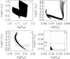 |
Fig. 1 a) All evolutionary tracks in the HR diagram; b) Evolutionary tracks falling in the error boxes from pre-main sequence to main sequence; c) Blow up the evolutionary tracks falling in the error boxes in the main sequence; d) The selected models falling in the error boxes. Error box A (5525 ± 12 K, 0.50 ± 0.006 L⊙) is denoted by crosses, error box B (5264 ± 100 K, 0.52 ± 0.03 L⊙) denoted by triangles, and error box C (5264 ± 100 K, 0.488 ± 0.010 L⊙) denoted by diamonds, respectively. |
The observational frequencies and the theoretical frequencies for model M1 & M2 before and after correction for near-surface offset, respectively.
We calculated many evolutionary tracks using Yale stellar evolution code (YREC; Demarque et al. 2008) by inputting different parameters shown in Table 2.
The mass range are M = 0.770–0.795 M⊙ with the increment value 0.005 M⊙. Initial heavy element abundance range are Zi (0.001–0.008) with the increment value 0.0005 and initial hydrogen abundance Xi (0.70–0.75) with the increment value 0.01. Energy transfer by convection is treated according to the standard mixing-length theory, and the boundaries of the convection zones are determined by the Schwarzschild criterion (see Demarque et al. 2008, for details of the YREC). We set the mixing length parameter α = 0.8–1.8 with the increment value 0.2. Using these parameter space, we created the model array. The initial zero-age main sequence (ZAMS) model used for τ Ceti is created from pre-main-sequence evolution calculations. These models are calculated using the updated OPAL equation-of-state tables EOS2005 (Rogers & Nayfonov 2002). We used OPAL high temperature opacities (Iglesias & Rogers 1996) supplemented with low temperature opacities from Ferguson et al. (2005). The NACRE nuclear reaction rates (Angulo et al. 1999) were used. The Krishna-Swamy Atmosphere T-τ relation is used for solar-like star (Guenther & Demarque 2000). All models included gravitational settling of helium and heavy elements using the formulation of Thoul et al. (1994).
Figure 1a shows that many evolutionary tracks cover all possible evolutionary status of τ Ceti. According to the above four error boxes, we select all the tracks crossing the error boxes shown in Fig. 1b. We only choose to study main-sequence models, which are shown in Fig. 1c. Meanwhile, we use the mass and radius to estimate the large separation according to Eq. (1) (Kjeldsen & Bedding 1995; Miglio et al. 2009a,b). Furthermore, using the temperature, luminosity, radius, and larger separation (refer to the values from Teixeira et al. 2009) as constrainst, we select the models of τ Ceti provided in Fig. 1d as candidates.  (1)We now consider a function that describes the agreement between the observations and the theoretical results
  (2)where C represents the quantities L/L⊙, Teff, R/R⊙, and [Fe/H]s and large frequency separation Δν, Ctheo represents the theoretical values, and Cobs represents the observational values listed in Table 1. The vector
  contain the errors in these observations, which are also given in Table 1. We also decided to adopt a large error (all errors are increased by a factor of 1.5), so that our calibration of the star is only weakly constrained by these values, which is not precisely determined. Figure 2a presents the values
  versus age t of selected models that are shown in Fig. 1d. We find that we cannot select an optimal model from Fig. 2a. From Fig. 2a, we find that it is difficult to select an optimal model depending mainly on the non-seismic constraints and Δν, which was estimated by simply scaling from solar value using Eq. (1). Hence, a detailed pulsation analysis are needed in the next step.
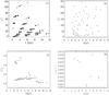 |
Fig. 2 a) |
4. Asteroseismic constraints of fundamental parameters
Using Guenther’s pulsation code (Guenther 1994), we calculate the adiabatic low-lp-mode frequencies, the large- and small- frequency separations (Δνn,l ≡ νn,l − νn−1,l and δνn,l ≡ νn,l − νn−1,l+2, defined by Tassoul 1980) of all the selected models. We compare the theoretical frequencies with the corresponding observational frequencies using the function 
 (3)where, N = 31 is the total number of modes, and
  and
and  are the theoretical and observed frequencies respectively, for each spherical degree l and the radial order n, where σ = 2 μHz (Teixeira et al. 2009) represents the uncertainty in the observed frequencies and values, plotted as function of age, are shown in Fig. 2b.
Since existing stellar models fail to accurately represent the near-surface layers of the solar-like stars, where the turbulent convection take place, the systematic offset between the observed and model frequencies appears. Furthermore, this offset between observed and best model frequencies turns out to be closely fitted by a power law (Christensen-Dalsgaard & Gough 1980; Kjeldsen et al. 2008; Metcalfe et al. 2009; Doǧan et al. 2009, 2010; Bedding et al. 2010; Christensen-Dalsgaard et al. 2010). In other words, this offset increases with increasing frequency shown in Fig. 3. This power law can be expressed using the equation ![Mathematical equation: \begin{equation} \nu_{\rm obs}(n)-r_{l}\nu_{\rm theo}(n)=a_{l}[\nu_{\rm obs}(n_{i})/\nu_{\rm max}]^{b}, \end{equation}](/articles/aa/full_html/2011/02/aa14886-10/aa14886-10-eq78.png) (4)where νobs are the observed frequencies of radial and non-radial order, νbest = rlνtheo(n) are the corresponding calculated frequencies of the best-fit model, and νmax is a constant frequency corresponding to the peak power in the spectrum, which is taken as 4490 μHz for τ Ceti and rl, al, and b are parameters described in detail by Kjeldsen et al. (2008), (for a different spherical degree l, the values of r and a are denoted by rl and al, respectively). For the Sun and a solar-like star, the exponent b = 4.90 is appropriate, as has been proven by many scientists. We use the Kjeldsen et al. (2008) prescription to correct the theoretical frequencies from near surface effects.
(4)where νobs are the observed frequencies of radial and non-radial order, νbest = rlνtheo(n) are the corresponding calculated frequencies of the best-fit model, and νmax is a constant frequency corresponding to the peak power in the spectrum, which is taken as 4490 μHz for τ Ceti and rl, al, and b are parameters described in detail by Kjeldsen et al. (2008), (for a different spherical degree l, the values of r and a are denoted by rl and al, respectively). For the Sun and a solar-like star, the exponent b = 4.90 is appropriate, as has been proven by many scientists. We use the Kjeldsen et al. (2008) prescription to correct the theoretical frequencies from near surface effects.
According to Eq. (4), we can use the following equation to obtain the corrected frequencies of models: ![Mathematical equation: \begin{equation} \nu_{\rm correct}(n)=r_{l}\nu_{\rm theo}(n)+a_{l}[\nu_{\rm obs}(n)/\nu_{\rm max}]^{b}. \end{equation}](/articles/aa/full_html/2011/02/aa14886-10/aa14886-10-eq89.png) (5)We define the function in a similar way to Eq. (3) as
(5)We define the function in a similar way to Eq. (3) as  (6)The values of , plotted as a function of age are shown in Fig. 2c. From Fig. 2c, we can see that the values of are lower than and their lowest values correspond to model ages from 8 to 10 Gyr. We conclude that the optimal model corresponds to the lower values of and r0 − 1. From Figs. 2c and 2d, we infer that only two models M1 and M2 can be accurately described by the observational constraints. The difference between the observed and uncorrected model frequencies of M1 and M2 are shown in Fig. 3. The uncorrected and corrected frequencies of the optimal models M1 and M2 and the observational frequencies are shown in Table 3.
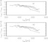 |
Fig. 3 The difference between observed and best-fit model frequencies, according to the left term of Eq. (4). Squares are used for l = 0 modes, diamonds for l = 1 modes, triangles for l = 2 modes, and circles for l = 3. Dotted lines show the power-law function, according to the right term of Eq. (4). |
To clearly compare all of the theoretical frequencies of the models with observational frequencies, we provide echelle diagrams of models M1 and M2 in Fig. 4. An Echelle diagram is a useful tool for comparing stellar models with observations. This diagram presents the mode frequencies along the ordinate axis, and the same frequencies modulo the large separations in abscissae. From Figs. 4a and 4d, it can be seen that the uncorrected theoretical frequencies are not closely in agreement with the observed frequencies. The corrected theoretical frequencies indicated by Eq. (5) fit perfectly the observation shown in Figs. 4b and 4e. Because the observed frequencies of orders n are not consecutive and the values of νobs(n) are very close to those of νtheo(n), we substitute the νtheo(n)/νmax for νobs(n)/νmax. Hence Eq. (5) becomes ![Mathematical equation: \begin{equation} \nu_{\rm correct}(n)=r\nu_{\rm theo}(n)+a[\nu_{\rm theo}(n)/\nu_{\rm max}]^{b}. \end{equation}](/articles/aa/full_html/2011/02/aa14886-10/aa14886-10-eq100.png) (7)From Figs. 4b, 4c, 4e, and 4f, it can be seen that corrected frequencies given by Eqs. (5) and (7) respectively are uniform and reproduce the observed frequencies perfectly. Furthermore, we can use the function to select the fitting model parameters. As we all know, the suitable model parameters correspond to the lowest values of , which can be clearly seen in Fig. 5. From Fig. 5, we can conclude that the mass is in the range 0.775−0.785 M⊙, α is in the range 1.6−1.8, Zi in 0.0065−0.0075, and Xi 0.73−0.75. Hence, the model parameters of τ Ceti can be constrained to within these narrow ranges. Finally, we list the model parameters and characteristics of models M1 and M2 in Table 4.
(7)From Figs. 4b, 4c, 4e, and 4f, it can be seen that corrected frequencies given by Eqs. (5) and (7) respectively are uniform and reproduce the observed frequencies perfectly. Furthermore, we can use the function to select the fitting model parameters. As we all know, the suitable model parameters correspond to the lowest values of , which can be clearly seen in Fig. 5. From Fig. 5, we can conclude that the mass is in the range 0.775−0.785 M⊙, α is in the range 1.6−1.8, Zi in 0.0065−0.0075, and Xi 0.73−0.75. Hence, the model parameters of τ Ceti can be constrained to within these narrow ranges. Finally, we list the model parameters and characteristics of models M1 and M2 in Table 4.
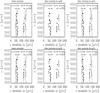 |
Fig. 4 Echelle diagrams for the optimal models M1 (upper panel) and M2 (lower panel). Left panel shows the case before applying near-surface corrections. Middle panel shows the case after applying near-surface corrections, according to Eq. (5). Right panel shows the case after applying near-surface corrections, according to Eq. (7). Open symbols refer to the theoretical frequencies, and filled symbols refer to the observable frequencies. Squares are used for l = 0 modes, diamonds for l = 1 modes, triangles for l = 2 modes, and circles for l = 3. The observable frequencies correspond to the average large separation about 170 μHz (see text for details). |
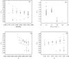 |
Fig. 5 a) |

Final model-fitting results for τ Ceti.
5. Discussion and conclusions
Using the asteroseismic analysis and the empirical frequency correction for the near-surface offset presented by Kjeldsen et al. (2008) to correct our theoretical frequencies, we have derived the optimal model of τ Ceti and now list our main conclusions:
-
1.
Using the latest asteroseismic observations, we have attemptedto construct the optimal model of τ Ceti. We have only considered the models M1 and M2 , which can closely describe the observations, as the optimal models. Furthermore, the model parameters of τ Ceti have been constrained to within narrow intervals by the function
,
where the mass is in the range
M = 0.775−0.785 M⊙, the mixing
length parameter in the range α = 1.6−1.8, the initial
metallicity in the range
Zi = 0.0065−0.0075, the initial
hydrogen abundance in the range
Xi = 0.73−0.75, and the age in the
range t = 8−10 Gyr. -
2.
We have found that the results of the non-asteroseismic observations (effective temperature and luminosity) inferred from spectroscopy are more accurate than those derived from interferometry for τ Ceti, because our optimal models are in the error boxes B and C derived from our spectroscopy results.
Acknowledgments
We are grateful to the anonymous referee for his/her constructive suggestions and valuable remarks that helped us to improve the manuscript. We also thank Professor Shaolan Bi and Dr. Linghuai Li for many useful comments and discussions. This work was supported by the support of Shandong Nature Science Foundation (ZR2009AM021), Dezhou University Foundation(402811), and supported by The Ministry of Science and Technology of the Peoples Republic of China through grant 2007CB815406, and by NSFC grants 10773003, 10933002, and 10978010.
References
- Arentoft, T., Kjeldsen, H., Bedding, T. R., et al. 2008, ApJ, 687, 1080 [NASA ADS] [Google Scholar]
- Angulo, C., Arnould, M., Rayet, M., et al. 1999, Nucl. Phys. A., 656, 3 [NASA ADS] [CrossRef] [Google Scholar]
- Bessell, M. S., Castelli, F., & Plez, B. 1998, A&A, 333, 231 [NASA ADS] [Google Scholar]
- Bedding, T. R., Butler, R. P., Kjeldsen, H., et al. 2001, ApJ, 549, L105 [NASA ADS] [CrossRef] [Google Scholar]
- Bedding, T. R., Kjeldsen, H., Butler, R. P., et al. 2004, ApJ, 614, 380 [NASA ADS] [CrossRef] [Google Scholar]
- Bedding, T. R., Butler, R. P., Carrier, F., et al. 2006, ApJ, 647, 558 [NASA ADS] [CrossRef] [Google Scholar]
- Bedding, T. R., Kjeldsen, H., Arentoft, T., et al. 2007, ApJ, 663, 1315 [NASA ADS] [CrossRef] [Google Scholar]
- Bedding, T. R., Kjeldsen, H., Campante, T. L., et al. 2010, ApJ, 713, 935 [NASA ADS] [CrossRef] [Google Scholar]
- Bouchy, F., & Carrier, F. 2002, A&A, 390, 205 [NASA ADS] [CrossRef] [EDP Sciences] [Google Scholar]
- Bouchy, F., Bazot, M., Santos, N. C., Vauclair, S., & Sosnowska, D. 2005, A&A, 440, 609 [NASA ADS] [CrossRef] [EDP Sciences] [Google Scholar]
- Bruntt, H., Bedding, T. R., Quirion, P.-O., et al. 2010, MNRAS, 405, 1907 [NASA ADS] [Google Scholar]
- Brown, T. M., Gilliland, R. L., Noyes, R. W., & Ramsey, L. W. 1991, A&A, 368, 599 [Google Scholar]
- Carrier, F., & Bourban, G. 2003, A&A, 406, L23 [NASA ADS] [CrossRef] [EDP Sciences] [Google Scholar]
- Carrier, F., & Eggenberger, P. 2006, A&A, 450, 695 [NASA ADS] [CrossRef] [EDP Sciences] [Google Scholar]
- Carrier, F., Bouchy, F., Kienzle, F., et al. 2001, A&A, 378, 142 [NASA ADS] [CrossRef] [EDP Sciences] [Google Scholar]
- Carrier, F., Bouchy, F., & Eggenberger, P. 2003, in Asteroseismology Across the HR Diagram, ed. M. J. Thompson, M. S. Cunha, & M. J. P. F. G. Monteiro (Kluwer), 311 [Google Scholar]
- Carrier, F., Eggenberger, P., D’Alessandro, A., & Weber, L. 2005a, New Astron., 10, 315 [NASA ADS] [CrossRef] [Google Scholar]
- Carrier, F., Eggenberger, P., & Bouchy, F. 2005b, A&A, 434, 1085 [NASA ADS] [CrossRef] [EDP Sciences] [Google Scholar]
- Carrier, F., Kjeldsen, H., Bedding, T. R., et al. 2007, A&A, 470, 1059 [NASA ADS] [CrossRef] [EDP Sciences] [Google Scholar]
- Carrier, F., Morel, T., Miglio, A., et al. 2010, Ap&SS, 328, 83 [NASA ADS] [CrossRef] [Google Scholar]
- Casagrande, L., Portinari, L., & Flynn, C. 2006, MNRAS, 373, 13 [NASA ADS] [CrossRef] [Google Scholar]
- Christensen-Dalsgaard, J., & Gough, D. O. 1980, Nature, 288, 544 [NASA ADS] [CrossRef] [Google Scholar]
- Christensen-Dalsgaard, J., Kjeldsen, H., Brown, T. M., et al. 2010, ApJ, 713, L164 [NASA ADS] [CrossRef] [Google Scholar]
- Chaplin, W. J., Appourchaux, T., Elsworth, Y., et al. 2010, ApJ, 713, L169 [NASA ADS] [CrossRef] [Google Scholar]
- Demarque, P., Guenther, D. B., Li, L. H., et al. 2008, Ap&SS, 316, 31 [NASA ADS] [CrossRef] [Google Scholar]
- De Ridder, J., Barban, C., Carrier, F., et al. 2006, A&A, 448, 689 [NASA ADS] [CrossRef] [EDP Sciences] [Google Scholar]
- Di Folco, E., Thvenin, F., Kervella, P., et al. 2004, A&A, 426, 601 [NASA ADS] [CrossRef] [EDP Sciences] [Google Scholar]
- Di Folco, E., Absil, O., Augereau, J.-C., et al. 2007, A&A, 475, 243 [NASA ADS] [CrossRef] [EDP Sciences] [Google Scholar]
- Doǧan, G., Brandão, I. M., Bedding, T. R., et al. 2009, Ap&SS, 328, 101 [Google Scholar]
- Doǧan, G., Bonanno, A., & Christensen-Dalsgaard, J. 2010, appear in the HELAS IV International Conference proceedings in Astronomische Nachrichten [Google Scholar]
- Eggenberger, P., Carrier, F., Bouchy, F., & Blecha, A. 2004a, A&A, 422, 247 [NASA ADS] [CrossRef] [EDP Sciences] [Google Scholar]
- Eggenberger, P., Charbonnel, C., Talon, S., et al. 2004b, A&A, 417, 235 [NASA ADS] [CrossRef] [EDP Sciences] [Google Scholar]
- Eggenberger, P., Carrier, F., & Bouchy, F. 2005, New Astron., 10, 195 [NASA ADS] [CrossRef] [Google Scholar]
- Eggenberger, P., Miglio, A., Carrier, F., et al. 2008, A&A, 482, 631 [NASA ADS] [CrossRef] [EDP Sciences] [Google Scholar]
- Ferguson, J. W., Alexander, D. R., Allard, F., et al. 2005, ApJ, 623, 585 [NASA ADS] [CrossRef] [Google Scholar]
- Gai, N., Bi, S. L., & Tang, Y. K. 2008, ChJAA, 8, 591 [NASA ADS] [Google Scholar]
- Gray, D. F., & Baliunas, S. L. 1994, ApJ, 427, 1042 [NASA ADS] [CrossRef] [Google Scholar]
- Grevesse, N., & Sauval, A. J. 1998, SSRv, 85, 161 [Google Scholar]
- Guenther, D. B. 1994, ApJ 422, 400 [NASA ADS] [CrossRef] [Google Scholar]
- Guenther, D. B., & Demarque, P. 2000, ApJ, 531, 503 [NASA ADS] [CrossRef] [Google Scholar]
- Guenther, D. B., Demarque, P., Kim, Y.-C., et al. 1992, ApJ, 387, 372 [NASA ADS] [CrossRef] [Google Scholar]
- Iglesias, C. A., & Rogers, F. J. 1996, ApJ, 464, 943 [NASA ADS] [CrossRef] [Google Scholar]
- Judge, P. G., Saar, S. H., Carlsson, M., & Ayres, T. R. 2004, ApJ, 609, 392 [NASA ADS] [CrossRef] [Google Scholar]
- Kallinger, T., Weiss, W. W., Barban, C., et al. 2010, A&A, 509, A77 [NASA ADS] [CrossRef] [EDP Sciences] [Google Scholar]
- Kervella, P., Thévenin, F., Morel, P., et al. 2004, A&A, 413, 251 [NASA ADS] [CrossRef] [EDP Sciences] [Google Scholar]
- Kjeldsen, H., & Bedding, T. R. 1995, A&A, 293, 87 [NASA ADS] [Google Scholar]
- Kjeldsen, H., Bedding, T. R., Baldry, I. K., et al. 2003, AJ, 126, 1483 [NASA ADS] [CrossRef] [Google Scholar]
- Kjeldsen, H., Bedding, T. R., Butler, R. P., et al. 2005, ApJ, 635, 1281 [NASA ADS] [CrossRef] [Google Scholar]
- Kjeldsen, H., Bedding, T. R., & Christensen-Dalsgaard, J. 2008, ApJ, 683, L175 [NASA ADS] [CrossRef] [Google Scholar]
- Li, L. H., Robinson, F. J., Demarque, P., Sofia, S., & Guenther, D. B. 2002. ApJ, 567, 1192 [NASA ADS] [CrossRef] [Google Scholar]
- Martić, M., Lebrun, J.-C., Appourchaux, T., & Korzennik, S. G. 2004a, A&A, 418, 295 [NASA ADS] [CrossRef] [EDP Sciences] [Google Scholar]
- Martić, M., Lebrun, J. C., Appourchaux, T., & Schmitt, J. 2004b, in SOHO 14/GONG 2004 Workshop, Helio- and Asteroseismology: Towards a Golden Future, ed. D. Danesy, ESA SP-559, 563 [Google Scholar]
- Metcalfe, T. S., Creevey, O. L., & Christensen-Dalsgaard, J. 2009, ApJ, 699, 373 [NASA ADS] [CrossRef] [Google Scholar]
- Metcalfe, T. S., Judge, P. G., Basu, S., et al. 2010, AAS Meeting 215, 424.16 [Google Scholar]
- Miglio, A., & Montalbán, J. 2005, A&A, 441, 615 [NASA ADS] [CrossRef] [EDP Sciences] [Google Scholar]
- Miglio, A., Montalbán, J., Eggenberger, P., et al. 2009a, AIP Conf. Proc., 1170, 132 [NASA ADS] [CrossRef] [Google Scholar]
- Miglio, A., Montalbán, J., Baudin, F., et al. 2009b, A&A, 503, L21 [NASA ADS] [CrossRef] [EDP Sciences] [MathSciNet] [Google Scholar]
- Mosser, B., Bouchy, F., Catala, C., et al. 2005, A&A, 431, L13 [NASA ADS] [CrossRef] [EDP Sciences] [Google Scholar]
- Pijpers, F. P. 2003, A&A, 400, 241 [NASA ADS] [CrossRef] [EDP Sciences] [Google Scholar]
- Pijpers, F. P., Teixeira, T. C., Garcia, P. J., et al. 2003, A&A, 406, L15 [NASA ADS] [CrossRef] [EDP Sciences] [Google Scholar]
- Provost, J., Martic, M., & Berthomieu, G. 2004, ESA SP-559, 594 [Google Scholar]
- Provost, J., Berthomieu, G., Martić, M., & Morel, P. 2006, A&A, 460, 759 [NASA ADS] [CrossRef] [EDP Sciences] [Google Scholar]
- Rogers, F. J., & Nayfonov, A. 2002, ApJ, 576, 1064 [Google Scholar]
- Robinson, F. J., Demarque, P., Li, L. H., et al. 2003, MNRAS, 340, 923 [NASA ADS] [CrossRef] [Google Scholar]
- Samadi, R., Georgobiani, D., Trampedach, R., et al. 2007, A&A, 463, 297 [NASA ADS] [CrossRef] [EDP Sciences] [Google Scholar]
- Soubiran, C., Katz, D., & Cayrel, R. 1998, A&AS, 133, 221 [NASA ADS] [CrossRef] [EDP Sciences] [Google Scholar]
- Stello, D., Chaplin, W. J., Basu, S., et al. 2010, MNRAS, 400, L80 [Google Scholar]
- Tang, Y. K., Bi, S. L., Gai, N., et al. 2008a, ChJAA, 8, 421 [NASA ADS] [Google Scholar]
- Tang, Y. K., Bi, S. L., & Gai, N. 2008b, New Astron., 13, 541 [Google Scholar]
- Tassoul, M. 1980, ApJS, 43, 469 [NASA ADS] [CrossRef] [Google Scholar]
- Teixeira, T. C., Kjeldsen, H., Bedding, T. R., et al. 2009, A&A, 494, 237 [NASA ADS] [CrossRef] [EDP Sciences] [Google Scholar]
- Thévenin, F., Provost, J., Morel, P., et al. 2002, A&A, 392, 9 [Google Scholar]
- Thoul, A. A., Bahcall, J. N., & Loeb, A. 1994, ApJ 421, 828 [NASA ADS] [CrossRef] [Google Scholar]
All Tables
The observational frequencies and the theoretical frequencies for model M1 & M2 before and after correction for near-surface offset, respectively.
All Figures
|
Fig. 1 a) All evolutionary tracks in the HR diagram; b) Evolutionary tracks falling in the error boxes from pre-main sequence to main sequence; c) Blow up the evolutionary tracks falling in the error boxes in the main sequence; d) The selected models falling in the error boxes. Error box A (5525 ± 12 K, 0.50 ± 0.006 L⊙) is denoted by crosses, error box B (5264 ± 100 K, 0.52 ± 0.03 L⊙) denoted by triangles, and error box C (5264 ± 100 K, 0.488 ± 0.010 L⊙) denoted by diamonds, respectively. |
| In the text | |
|
Fig. 2 a) |
| In the text | |
|
Fig. 3 The difference between observed and best-fit model frequencies, according to the left term of Eq. (4). Squares are used for l = 0 modes, diamonds for l = 1 modes, triangles for l = 2 modes, and circles for l = 3. Dotted lines show the power-law function, according to the right term of Eq. (4). |
| In the text | |
|
Fig. 4 Echelle diagrams for the optimal models M1 (upper panel) and M2 (lower panel). Left panel shows the case before applying near-surface corrections. Middle panel shows the case after applying near-surface corrections, according to Eq. (5). Right panel shows the case after applying near-surface corrections, according to Eq. (7). Open symbols refer to the theoretical frequencies, and filled symbols refer to the observable frequencies. Squares are used for l = 0 modes, diamonds for l = 1 modes, triangles for l = 2 modes, and circles for l = 3. The observable frequencies correspond to the average large separation about 170 μHz (see text for details). |
| In the text | |
|
Fig. 5 a) |
| In the text | |
Current usage metrics show cumulative count of Article Views (full-text article views including HTML views, PDF and ePub downloads, according to the available data) and Abstracts Views on Vision4Press platform.
Data correspond to usage on the plateform after 2015. The current usage metrics is available 48-96 hours after online publication and is updated daily on week days.
Initial download of the metrics may take a while.