| Issue |
A&A
Volume 526, February 2011
|
|
|---|---|---|
| Article Number | A20 | |
| Number of page(s) | 13 | |
| Section | The Sun | |
| DOI | https://doi.org/10.1051/0004-6361/201014617 | |
| Published online | 15 December 2010 | |
Equatorial coronal holes, solar wind high-speed streams, and their geoeffectiveness⋆
1
Department of GeophysicsFaculty of Science, University of
Zagreb, Horvatovac
95, 10000
Zagreb, Croatia
e-mail: This email address is being protected from spambots. You need JavaScript enabled to view it.
2
Hvar Observatory, Faculty of Geodesy, University of
Zagreb, Kačićeva
26, 10000
Zagreb,
Croatia
3
Institute for Physics, University of Graz, Universitätsplatz
5, 8010
Graz,
Austria
Received: 31 March 2010
Accepted: 9 October 2010
Abstract
Context. Solar wind high-speed streams (HSSs), originating in equatorial coronal holes (CHs), are the main driver of the geomagnetic activity in the late-declining phase of the solar cycle.
Aims. We analyze correlations between CH characteristics, HSSs parameters, and the geomagnetic activity indices, to establish empirical relationships that would provide forecasting of the solar wind characteristics, as well as the effect of HSSs on the geomagnetic activity in periods when the effect of coronal mass ejections is low.
Methods. We apply the cross-correlation analysis to the fractional CH area (CH) measured between central meridian distances ± 10°, solar wind parameters (flow velocity V, proton density n, temperature T, and the magnetic field B), and the geomagnetic indices Dst and Ap.
Results. The cross-correlation analysis reveals a high degree of correlation between all studied parameters. In particular, we show that the Ap index is considerably more sensitive to HSS and CH characteristics than Dst. The Ap and Dst indices are most tightly correlated with the solar wind parameter BV2.
Conclusions. From the point of view of space weather, the most important result is that the established empirical relationships provide a few-days-in-advance forecasting of the HSS characteristics and the related geomagnetic activity at the six-hour resolution.
Key words: Sun: corona / solar-terrestrial relations / solar wind
Appendices, Figs. 9–14, and table 4 are only available in electronic form at http://www.aanda.org
© ESO, 2010
1. Introduction
Solar wind high-speed streams (HSSs), originating from equatorial coronal holes (CHs), and the associated co-rotating interacting regions (CIRs) formed in front of HSSs (e.g., Gosling 1996, and references therein) cause medium-level, long-lasting, recurrent geomagnetic activity (e.g., Nolte et al. 1976; Vršnak et al. 2007b, and references therein). The geomagnetic effects are caused by the southward component of the interplanetary magnetic field (Bs) related to Alfvénic fluctuations within CIR/HSS structures (e.g., Schwenn 1983; Tsurutani & Gonzalez 1987; Tsurutani et al. 2004). Consequently, the most geoeffective region is expected to be the magnetic field compression within the CIR, where the field is strong and fluctuations are amplified.
Thus, forecasting the properties of HSS/CIRs is a central concern of space weather. Two methods are currently applied. The heliospheric MHD numerical codes like ENLIL (e.g., Lee et al. 2009; Odstrcil & Pizzo 2009, and references therein), or empirical/numerical hybrid models (e.g., HHMS; Detman et al. 2006) predict the basic physical parameters of the solar-wind, using synoptic solar magnetic field data as the model input. On the other hand, purely empirical methods provide forecasting of the solar wind characteristics at the Earth by utilizing relationships between the CH characteristics and the properties of HSSs (Nolte et al. 1976; Robbins et al. 2006; Vršnak et al. 2007a; Luo et al. 2008; Abramenko et al. 2009; Obridko et al. 2009). The empirical approach also enables a direct forecasting of the geomagnetic activity (Vršnak et al. 2007b).
In this paper, we built upon the empirical method proposed by Vršnak et al. (2007a,b) by increasing the time “resolution” from one-day to six-hour intervals. In a preliminary analysis, we tested various options, and found that a six-hour resolution is the optimal one, because when shorter intervals are applied the results do not change much but the noise level increases. Furthermore, we extend the study by performing an analysis of various combined solar wind parameters, and beside the geomagnetic Dst index we include also the Ap index.
Thus, there are two goals of the paper. The first is to analyze the correlation of indices Dst and Ap with the HSS/CIR parameters (such as magnetic field B, velocity V, a measure of the convective electric field VB, and the Poynting flux VB2) to learn in more detail how different magnetospheric current systems respond to the HSS/CIR-related solar-wind disturbances. The second is to prepare an empirical tool for predicting the HSS/CIR characteristics and forecasting the related geomagnetic activity.
In Sect. 2, we present the data. The correlations of the solar wind parameters with the geomagnetic indices are analyzed in Sect. 3, whereas in Sect. 4 we present a procedure that can be used for the forecasting of the HSS/CIR characteristics and the level of the geomagnetic activity based on CH measurements. The results are discussed in Sect. 5. Details of the cross-correlation analysis are provided in Appendix A, whereas in Appendix B we present some intriguing aspects of correlations between various solar wind parameters.
2. Data
Our study is based on the following data sets:
-
solar wind parameters (density n, temperature T, velocity V, and the magnetic field strength B);
-
fractional area CH of coronal holes;
-
geomagnetic indices Dst and Ap.
We focus on a period in the declining phase of the solar cycle No. 23, when the coronal mass ejection (CME) activity was very low and the solar wind was modulated primarily by HSSs. As in the papers by Vršnak et al. (2007a,b) and Temmer et al. (2007), we consider the period from 25 January 2005 to 5 May 2005 (day-of-year, DOY = 25−125).
The solar wind data were obtained from the Solar Wind Electron Proton and Alpha Monitor (SWEPAM; McComas et al. 1998) and the magnetometer instrument (MAG; Smith et al. 1998) onboard the Advanced Composition Explorer (ACE; Stone et al. 1998)1.
Solar coronal-hole fractional areas were determined from soft X-ray images acquired by the Soft X-ray Imager (SXI; Hill et al. 2005; Pizzo et al. 2005) onboard the GOES-12 spacecraft2. For our purposes, we used four SXI coronal images per day taken around 0, 6, 12, and 18 UT. In measuring the CH areas, we applied a fixed threshold to the calibrated SXI coronal hole images of 0.15 DN s-1. All pixels below this threshold (identified as coronal hole pixels) within a specified region of the solar disk were summed and divided by the total number of pixels of the considered region to evaluate the fractional area CH covered by coronal holes (for details, see Vršnak et al. 2007a). We determined the fractional area CH in the central-meridian slice, extending from the central meridian distance −10° to + 10°.
Planetary geomagnetic activity index Ap is a measure of the daily level of the mid-latitude magnetic activity. It is derived from a range of geomagnetic field variations over a period of 3 h from measurements provided by 13 geomagnetic observatories between 44° and 60° northern or southern geomagnetic latitudes3.
The storm-time disturbance index Dst, represents the axially symmetric disturbance magnetic field at the dipole equator on the Earth’s surface. Any decrease in Dst is mainly due to the ring current, while positive variations in Dst are caused by the compression of the magnetosphere produced by the increase in solar wind dynamic pressure. The Dst index is derived from hourly scalings of the horizontal magnetic field variations measured at four low-latitude geomagnetic observatories4.
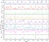 |
Fig. 1 Time series (6-h data resolution) of CH (fractional area), T(K), n(cm-3), B(nT), V(km s-1), BV, Dst(nT), and Ap(nT), from top to bottom, respectively. The time is expressed in the day-of-year form, DOY, for 2005. |
The six-hour running means of Dst are evaluated by averaging hourly values in the range of ± 3 h centered at 0, 6, 12, and 18 UT. We note that Ap index is given as the three-hourly-value, so the time window of of ± 3 h contains only three values for averaging.
Time series of CH, T, n, B, V, Dst, and Ap are shown in Fig. 1. We performed the spectral analysis and found period of 9.1 days for all quantities (see also Crowley et al. 2008; Lei et al. 2008a,b,c), which corresponds to 1/3 of the solar synodic rotation period. The periodicity is a consequence of three long-lived equatorial CHs separated in longitude by ≈ 120° (Vršnak et al. 2007a,b; Temmer et al. 2007).
In the analyzed period, these three coronal holes passed across the central meridian 11 times, resulting in 11 HSS/CIR structures at 1 AU (enumerated in Fig. 1; see also Table 1 of Vršnak et al. 2007a). The CIRs are seen as the density and magnetic field bumps ahead of HSSs.
In Fig. 2, we present a close-up of HSS No. 11 (DOY = 118−125) to illustrate in more detail a typical relationship between the behavior of the geomagnetic activity indices and the HSS/CIR-related solar-wind properties. Figure 2a shows that the Ap peaks and Dst dips appear at the frontal side of HSS (rise of the solar-wind speed), closely related to the CIR magnetic field compression. Moreover, the graph shows that the Ap peak appears during the decreasing phase of Dst, i.e., the Dst dip is delayed with respect to the Ap peak. This is emphasized in Fig. 2b where Ap(t) is compared to the change rate in Dst (ΔDst represents the change of Dst over the 6-h intervals). The graph shows that, within the considered time resolution, the peaks of Ap and ΔDst are contemporaneous (for a similar relationship between Dst and AE activity, see Gonzalez et al. 1994, and references therein). Furthermore, both peaks are contemporaneous with peaks of the product VB. This implies that Ap and VB behave as a derivative of the Dst, or more accurately, that Dst represents a cumulative consequence of VB, whereas Ap is a direct effect of VB. This behavior is more or less repeated in all HSS/CIRs in the analyzed period.
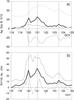 |
Fig. 2 Close-up of the interval DOY = 118−125 (HSS No. 11): a) development of Ap [nT] (bold-black) and Dst [nT] (thin-black) compared to the variation in the solar wind speed V [km s-1/10] (dashed) and the magnetic field B [nT] (bold-gray); b) Ap (bold-black) compared to the change rate of Dst (ΔDst, thin-black) and the product BV (bold-gray). |
3. Cross-correlations
In the following, we investigate the relationship between various solar wind parameters (n, B, T, V), fractional CH area CH, and the geomagnetic indices Ap and Dst, by applying the cross-correlation analysis. All cross-correlation functions (presented in graphs given in Appendix A) are derived up to a time lag of ±10 days, with a step of 6 h (data resolution) in all investigated cases. The time lags are always expressed in days. Negative lag between two quantities, e.g., V and Ap, hereinafter denoted as the V − Ap correlation, means that V is delayed with respect to Ap.
3.1. Cross-correlation between solar wind parameters and geomagnetic indices
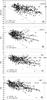 |
Fig. 3 Correlations V–Dst, B–Dst, BV − Dst,and BV2 − Dst. In panels b) − d) we separated the data points characterized by v > 450 km s-1 (circles), from those having v < 450 km s-1 (black dots). The linear least squares fit parameters, the correlation coefficient R, and the applied time lag Δt are shown in the insets; in panels b) − d) the fit parameters are shown only for the v > 450 km s-1 data (bold lines); dashed lines represent the fits for the v < 450 km s-1 data, dotted lines represent the results from Richardson & Cane (2010). |
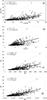 |
Fig. 4 Correlations V–Ap, B–Ap, BV–Ap, and BV2 − Ap. In panels b) − d) we separated the data points characterized by v > 450 km s-1 (circles), from those having v < 450 km s-1 (black dots). The linear least squares fit parameters, the correlation coefficient R, and the applied time lag Δt are presented in the insets; in panels b) − d), the fit parameters are for the v > 450 km s-1 data (bold line). Dashed lines are fits for the v < 450 km s-1 data; dotted lines represent an estimate of the upper limit. |
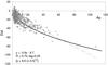 |
Fig. 5 Correlation between Dst and Ap, where Dst is delayed by 0.25 days. Parameters of the linear least square fit (dashed line) are given in the inset. Bold curve represents the function |
We calculated the cross-correlation functions for all combinations of solar-wind parameters and the geomagnetic indices Dst and Ap. The cross-correlation functions showing the highest correlation coefficients are presented in Appendix A.
In Figs. 3 and 4, the corresponding scatter plots for the highest-correlation time-lag are presented for the most tightly correlated parameters. The most relevant correlations are listed in Table 1 where the time lags Δt, the corresponding linear least squares fit parameters a and b, and the correlation coefficient R are presented. A given “X − Y” correlation corresponds to the linear form Y(t) = aX(t∗) + b, where X(t∗) represents the value of X that occurred Δt days before the true value of Y(t), i.e., t∗ is the “retarded time”, t∗ = t − Δt.
Inspecting Table 1 one finds that in the case of the Dst index, the highest correlation coefficient (R = 0.58) is found between Dst and BV2, which are anti-correlated, with the time delay of Δt = 0.25 d. Similar, but slightly lower, correlation coefficients are obtained for V − Dst and BV − Dst relationships. We note that the Dst dip is contemporaneous with the V peak, whereas it is delayed with respect to all other solar wind parameters.
The data presented in Fig. 3 can be straightforwardly compared with the results presented by Richardson & Cane (2010). We considered the total magnetic field, while they considered the southward component of the magnetic field, Bs. They analyzed a set of geomagnetic storms caused by magnetic clouds and found a high degree of correlation between Dst and solar wind parameters Bs, V, and BsV (R = 0.89, 0.54, and 0.90, respectively; the corresponding regression lines are drawn by dotted lines)5. The slopes of Dst(Bs) and Dst(BsV) found by Richardson & Cane (2010) are steeper than our Dst(B) and Dst(BV) slopes, which is to be expected, since Bs < B: the regression lines from Richardson & Cane (2010) are close to the lower limit edge of our Dst(B) and Dst(BV) data scatter. On the other hand, the steeper Dst(V) slope in Richardson & Cane (2010) cannot be explained in this manner; it indicates that CIRs affect the geomagnetic field in a somewhat different manner than CMEs: at the same flow speed, CMEs are far more effective.
In addition, our CIR Dst–V correlation can be compared with the Dst − V correlations of MCs and non-MCs as reported by Gopalswamy (2010). He studied the major storms of solar cycle 23 and found that the CMEs resulting in MCs exibit a strong Dst − V correlation (R = −0.72), while CMEs that cause non-MCs exibit a very weak correlation (R = −0.14). For CIR storms analysed in our study, the Dst − V correlation (R = 0.54) is weaker than for MCs, but much stronger than for non-MCs.
Interestingly, for the intense CIR storms within the cycle 23, Gopalswamy (2008) found a much weaker correlation between both V and BV, and Dst (R < 0.3).
The data-point distribution in Fig. 3b shows that the moderate storm level (Dst below −50 nT) can be achieved only if magnetic field is strong enough, i.e., it has to be stronger than 5 nT. A storm can become intense (Dst < −100 nT) only if B > 10 nT. These values are consistent with previous estimates of the lower limit to the southward component of the magnetic field Bs (see Gonzalez et al. 1994, and references therein).
When comparing the magnetic content of CIRs with the MC and non-MC magnetic content, Gopalswamy (2008) found that the total magnetic field strength for CIRs, MCs and non-cloud ICMEs is as high as 19 nT, 23 nT and 20 nT, respectively (see Fig. 12 in his work). The magnetic content of CIRs in our study reaches the maximum value of 16 nT.
For the Ap index, the strongest correlation is found is between Ap and BV2, where Δt = 0 and the correlation coefficient R = 0.77. The peak of Ap is also contemporaneous with the peak of BV and B2V. Finally, we fitted the Ap(V) dependence using a quadratic function of the form Ap = aV2 + b (see, Crooker et al. 1977), and we got Ap = 7 × 10⁻⁵V2 − 5.4, which is quite close to the relationship found by Crooker et al. (1977) for the yearly-averaged values. We note that the difference between the correlation coefficients of the linear and quadratic fit is not significant (there being R = 0.66 and R = 0.67, respectively).
The data in panels a) − c) of Figs. 3 and 4 are presented separately for v > 450 km s-1 (circles) and v < 450 km s-1 (black dots). Comparing the correlations for the case v > 450 km s-1 (check the inset in Figs. 3 and 4) with those obtained for the complete sample (Table 1), one finds that the correlation coefficients remain at more or less the same level. However, the slopes of regression lines become steeper. On the other hand, for v < 450 km s-1 data, the correlation coefficients become significantly lower and the slope of regression lines are less steep. This clearly indicates that high speed streams are more geoeffective than either fluctuations within the slow solar wind or frontal parts of corotating interacting regions where the wind speed is still low. In other words, magnetic field compressions and higher wind speed are both needed to enhance the geomagnetic activity.
Indices Ap and Dst are anti-correlated with R = 0.75 for the delay of Dst after Ap of Δt = 0.25 (Fig. 5 and the last row of Table 1). Although the correlation-coefficient is high, we note that these two indices show considerable differences. For example, Dst can attain values as low as −40 nT, without practically any signal in Ap index.
The explanation can be found in the different behavior of the Ap and Dst variations (see, Fig. 2), namely that the Dst variation is characterized by the recovery phase whose duration is longer than the duration of the Ap peak. Thus, although the Ap index already attains low values, the Dst is still quite far from Dst = 0.
The difference can also be seen by comparing Figs. 3 and 4, which have a different types of data scatter. Inspecting graphs in Fig. 4, we find that the distribution of data-points exibit a triangular pattern, where the lower limit of Ap is approximately aligned with Ap = 0 for a wide range of values characterizing the solar-wind parameters (x-axis). On the other hand, the upper limit of Ap is clearly dependent on the solar-wind parameters. For example, the upper limits can be expressed approximately as Ap ≈ 0.3(V − 300), Ap ≈ 12(B − 2), Ap ≈ 6(BV − 500), and Ap ≈ 3(BV2 − 0.2), where V is expressed in km s-1 and B in nT.
The described “triangular distribution” of data points in Fig. 4 means that large values of V, B, BV, or BV2 do not necessarily imply that a high level of geomagnetic activity is beeing measured by Ap. On the other hand, high values of Ap cannot correspond to low values of the afore mentioned solar-wind parameters. In contrast to Ap, the Dst-related correlations presented in Fig. 3 do not show such a pronounced “triangular” shape, i.e., the upper limit (Dst = 0) is not so sharply defined.
Finally, the distribution of data points in Fig. 5 indicates that the relationship Dst(Ap) might not be linear. Thus, we also tried a quadratic fit to the Ap(Dst) data, and the correlation coefficient increased to R = 0.83, with Ap = 0.015Dst2 + 0.078Dst + 4. The same correlation coefficient was found for the reduced quadratic fit, Ap = 0.013Dst2 + 3.5 (corresponding to 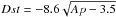 , shown in Fig. 5). This implies that Ap can be represented as a quadratic function of Dst.
Relationships between geomagnetic indices and solar wind parameters.
3.2. The relationship to coronal holes
 |
Fig. 6 Correlations CH–V, CH–n, CH–B, and CH–T. The linear least squares fit parameters, correlation coefficient R, and the applied time lag Δt are presented in the insets. |
The cross-correlation functions for the relationships between coronal hole fractional area, CH, and the solar wind parameters are shown in Appendix A.
The corresponding scatter plots are shown in Fig. 6, and the relationships are summarized in Table 2, where we show the linear least squares fit parameters, the correlation coefficients R, and time lags Δt. The coronal hole fractional area is more tightly correlated with the solar wind velocity (R = 0.59 and Δt = 3.75 days).
This result agrees with earlier findings of Krieger et al. (1973), Neupert & Pizzo (1974), Nolte et al. (1976). In the study by Nolte et al. (1976), a very high correlation (0.96) between coronal hole area and maximal velocity in the associated stream was obtained. The larger scatter in the data presented in our Fig. 6 (top panel), is due to: (a) usage of the fractional coronal hole area in the central meridian slice, not the entire CH area; (b) solar wind speed depends not only on the coronal hole size, but also on the magnetic field strength and the magnetic flux expansion rate (Fujiki et al. 2005).
Inspecting Table 2, we find that the average delay between the CH(t) signal and the CIR-related n(t) variation is only 0.75 days (consistent with the results presented by Vršnak et al. 2007a). At first sight, this might be surprising since the solar-wind transit time is expected to be at least 2−3 days. A similar result is found for the estimated delay of B(t), where Δt = 1.75 d. To explain such short delays we have to take into account the spatial extent of coronal holes as well as the CIR-compression having formed at the frontal side of the HSS (Gosling 1996), i.e., it maps on to the leading edge of the coronal hole. From Fig. 1, one can see that the rise in the CH(t) signal from the beginning to the peak lasts from 1 to 3 days. In other words, the leading edge of the CH has passed over the central meridian 1−3 days earlier than its central regions, which is a result of the large spatial extent of CHs. Thus, for the largest CHs, at the moment when the “center” of CH passes over the central meridian, the CH leading edge is already quite far to the west. In these cases, the bump in n can be almost contemporaneous with the peak of CH (e.g., CIR No. 6 around DOY = 73; see also Fig. 1 in Vršnak et al. 2007a). In the case of a small CH, the delay tends to be longer, generally around 2−3 days. Thus, we examined the delays of n bumps relative to the onset of the rise in the CH signal, and found out that the delays range between 2 and 4 days, with the average value of 3.6 ± 1.1 days.
Relationships between solar wind parameters and CH.
In this respect, we note that sometimes, depending on the shape of the CH area, the CH(t) signal displays a complex structure (see e.g., the double-peaked CH bump related to HSS No. 10, DOY = 107−110). This probably results in a complex evolution of the HSS/CIR structure in the interplanetary space, which may result in an apparently unexpected, early appearance of the CIR-related density compression.
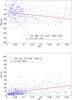 |
Fig. 7 Correlations CH–Dst and CH–Ap; the linear least squares fit parameters, the correlation coefficient R, and the applied time lag Δt are presented in the insets. |
Figure 7 shows the correlations CH–Dst and CH–Ap (the corresponding cross-correlation functions are shown in Appendix A). The time lags and the linear least squares fit parameters are given in Table 3. We note that the correlation between Ap and CH is much tighter than between Dst and CH (R = 0.43 and R = −0.27, with Δt = 3.0 and Δt = 3.75, respectively).
4. Forecasting the solar wind parameters and geomagnetic indices
Linear regression coefficients a and b given in Table 3 can be employed to predict the solar wind parameters from the CH data in periods of low CME activity. In this respect, we note that since the linear regression analysis is based on the least squares procedure, its application leads to an underestimate of the predicted variation-amplitudes (see thin black line in Fig. 8). The main cause of this effect is the timing mismatch of some of the peaks in the two curves (for details see Vršnak et al. 2007a).
Thus, since we are mainly interested in reproducing the real amplitudes (peak values), we subjectively “corrected” the linear regression coefficients to fit more closely the amplitudes themselves. In this procedure, it is necessary to decrease the value of parameter b, so that the “background” slow solar wind comes closer to the observed values, as well to increase parameter a in order to stretch the amplitudes (see Figs. 8a−d).
Relationship between CH and geomagnetic indices.
Thus, we did not directly apply the relationships based on the linear least squares fit (parameters a and b as given in Table 2), but used them as a starting point for finding the most appropriate values of these parameters. After trying different combinations, we determined the optimal parameters/relationships that more properly reproduce the amplitudes. These parameters are given in Table 3 and are denoted as acorr and bcorr. Curves obtained with these coefficients are shown as a thick black curve in Figs. 8a−d.
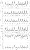 |
Fig. 8 a)–d) Comparison of the observed solar wind parameters with the calculated values. The observed data are inicated by the thick gray line, calculated values (using linear regression parameters a and b as given in Table 2) are drawn by thin black line, and the amplitude-optimized “predicted” values (using linear regression parameters acorr and bcorr as given in Table 2) are drawn by thick black line. e) − f) Comparison of the measured values of the geomagnetic indices Dst and Ap with the calculated values. The observed data are delineate by the thick gray line, values calculated for the N-polarity CHs are drawn by thick-dashed line, and S-polarity CHs are indicated by thick-black line. See text for details. |
The empirical relationship between the CH fractional areas and indices Dst and Ap also opens the possibility of predicting the level of the HSS-related geomagnetic activity a few days in advance. In Figs. 8e−f, we present the observed values of Dst and Ap (bold-gray line) and the values calculated using the relationships ![Mathematical equation: \begin{equation} Dst =( -80 \pm 30\times \cos \lambda) \times [CH(t^*)]^{1/2} \end{equation}](/articles/aa/full_html/2011/02/aa14617-10/aa14617-10-eq139.png) (1)and
(1)and ![Mathematical equation: \begin{equation} Ap = (120 \pm 60\times \cos \lambda) \times [CH(t^*)] \end{equation}](/articles/aa/full_html/2011/02/aa14617-10/aa14617-10-eq140.png) (2)(for details regarding Dst predictions see, Vršnak et al. 2007b), where, λ is the ecliptic longitude and ± applies as plus for CHs of positive magnetic polarity and as minus for negative polarity CHs. For forecasting purposes, λ can be estimated using λ = 2π(t − 81) / 365, where the time t is expressed as DOY (for details see, Vršnak et al. 2007b). The “predicted” values of geomagnetic indices are based on the CH areas measured at the retarded time t∗ = t − Δt, where Δt = 3.75 and Δt = 3 are assumed for Dst and Ap, respectively.
(2)(for details regarding Dst predictions see, Vršnak et al. 2007b), where, λ is the ecliptic longitude and ± applies as plus for CHs of positive magnetic polarity and as minus for negative polarity CHs. For forecasting purposes, λ can be estimated using λ = 2π(t − 81) / 365, where the time t is expressed as DOY (for details see, Vršnak et al. 2007b). The “predicted” values of geomagnetic indices are based on the CH areas measured at the retarded time t∗ = t − Δt, where Δt = 3.75 and Δt = 3 are assumed for Dst and Ap, respectively.
The employed “forecast” relationships differ from those proposed by Vršnak et al. (2007a,b) because of the higher amplitude values found in our 6-h data resolution, which are smoothed in 24-h data used in their study.
5. Discussion and conclusions
We have analyzed the relationship between solar wind parameters, coronal hole areas CH, and geomagnetic Dst and Ap indices for the period of low CME activity. The results are summarized as follows:
-
1.
With 6-h (1/4 day) data resolution, we obtained good correlations between all studied parameters. This allows us to evaluate average time delays Δt more accurately than in Vršnak et al. (2007a). A higher time resolution results in too large amounts of noise, so we consider the 6-h resolution as the optimal one.
-
2.
Ap and Dst are most tightly correlated with the solar-wind parameter-combination BV2 (R = 0.77 and R = −0.58, respectively). The corresponding delays are Δt = 0 days and Δt = 0.25. The indices Ap and Dst are correlated with R = −0.75, Dst being delayed for Δt = 0.25 days.
-
3.
The relationship Ap(Dst) can be represented by a quadratic dependence, with Dst being delayed on average for 0.25 days. The peaks of Ap are contemporaneous with the peaks of the product BV, whereas at the same time Dst displays the most sharpest decrease towards minimum.
-
4.
Values of Ap are more strongly correlated with CH then Dst (R = 0.43 and −0.27, respectively). The Dst dip lags after the CH peak for 3.75 days, while the Ap peak appears three days after the CH peak.
-
5.
We have developed a procedure that allows a several-days-in-advance prediction of the solar wind parameters near the Earth, as well as the level of the HSS/CIR-related geomagnetic activity, from the CH observations, at a six-hour resolution.
The tightest correlation between both considered geomagnetic indices, Ap and Dst, is found with BV2. The Ap(BV2) relationship is quite similar to the relationship found by Crooker et al. (1977) for the yearly-averaged data. This behavior shows that the combination of the solar-wind speed and magnetic field is essential to the process of energy transfer from the solar wind to the magnetosphere.
The physical mechanism behind the Ap(BV2) relationship is not entirely clear. For example, Ahluwalia (2000) noted that the physical unit for BV corresponds to the force per unit charge and that of BV2 to the power per unit charge. However, this does not explain the physical background of processes that lead to the situation where the geomagnetic activity indices have the tightest correlation with the product BV2.
According to the basic consideration of the energy transfer from the solar wind to the magnetosphere, the geomagnetic activity is forced by the magnetic reconnection near the nose of the magnetosphere (Siscoe & Crooker 1974). Thus, it is clear that the product BV related to the electric field in the current sheet, as well as the Poynting flux VB2, both play an important role in determining the level of the geomagnetic activity (e.g., Perreault & Akasofu 1978; Kan & Lee 1979, and references therein).
In this respect, we note that Kan & Lee (1979) have shown that the power delivered by the “solar wind dynamo” is proportional to B2V2. Our data indeed show that the Ap(BV) relationship, when expressed in the form Ap = a(BV)2 + b, has the correlation coefficient of R = 0.72 at Δt = 0 (Table 2). For the analogous relationship with Dst, we get R = 0.51 at Δt = +0.5.
However, this still does not explain the dominant correlation of geomagnetic indices with the parameter BV2, which obviously requires an additional explanation. One possibility is that this parameter represents the product of the induced electric field BV and the merging velocity V. The first term determines the electric field in the current sheet that accelerates particles, whereas the V term is related to the flow of particles entering into the current sheet.
The Ap index has a stronger correlation with all studied parameters than Dst does, i.e., it reacts to HSSs more directly than Dst (see also Verbanac et al. 2010). This implies that Ap is more sensitive to Alfvénic fluctuations in the solar wind high-speed streams (Tsurutani et al. 1995) than the Dst index.
Finally, we note that as a side result of our analysis we found two empirical invariants in the solar wind parameters. The value of V2, multiplied by the density n measured one day earlier, is approximately constant. Similarly, the solar wind speed V, multiplied by the magnetic field B measured 2.25 days earlier, is also approximately constant. Although at the moment we cannot offer a physical explanation, we consider this finding as potentially very important for understanding of the time/spatial structure of the high-speed streams.
Online material
Appendix A: Cross–correlation functions
In Figs. 9 − 13, we present the cross-correlation functions between different parameters, which we used to perform the correlation scatter plots presented in the paper. All cross-correlation functions are derived up to a time lag of ±10 days, with a step of 6 h (data resolution) in all investigated cases. The time lags are always expressed in days. Negative lag between two quantities, e.g., V and Ap, hereinafter denoted as the V − Ap correlation, means that V is delayed with respect to Ap.
Appendix B: Correlation between solar-wind parameters
We calculated the cross-correlation functions for all combinations of V, T, n, and B. In Figs. 9 and 14, the cross-correlation functions and the scatter plots for the highest-correlation-coefficient time-lag are presented for the most tightly correlated combinations. All considered correlations are listed in Table 4 where the time lags Δt, the corresponding linear least squares fit parameters a and b, and the correlation coefficient R are presented. A given “X − Y” correlation corresponds to the linear form Y(t) = aX(t∗) + b, where X(t∗) represents the value of X that occurred Δt days before the actual value of Y(t), i.e., t∗ is the “retarded time”, t∗ = t − Δt.
Table 4 shows that the most tightly correlated parameters are V and T, having the correlation coefficient R = 0.8, when V is delayed after T for Δt = 0.25 days. Furthermore, Fig. 9 shows that in the V − n and V − B case, the correlation coefficients are higher when the parameters are anti-correlated (the negative correlation coefficient in Table 4). This reflects the main physical property of HSSs, which is a depleted density and magnetic field in the stream itself. The anti-correlations are most significant for the time lags Δt = 0.75 d and Δt = 2.25 d, respectively, meaning that the dips of B and n are delayed with respect to the peak of V. The positive correlations of both the V − B and V − n relationships and their negative time lags (peaks of n and B preceding the peak of V by 2.5 d and 1.75 d), are related to the magnetic field and density compression in the “interacting region” at the frontal edge of HSSs. We note that the time lag in the n − B correlation is Δt = + 0.5 d, meaning that the peak of B is delayed with respect to the peak in n.
The distribution of data points in V–n and V–B graphs in Figs. 14b and c shows two “branches”, one almost horizontal and another almost vertical. The vertical one corresponds to the slow solar wind (V ≈ 300−400 km s-1), and the horizontal one to the fast solar wind (V > 400 km s-1 and low values of n and B). If fitted by the power-law, the relationships are given by n = 1.4 × 10⁶ × V−2.0 ± 0.1, and B = 4710 × V−1.1 ± 0.1, with the correlation coefficients R = 0.69 and R = 0.58, respectively. Although the applied power-law fit is obviously more appropriate than the linear fit, it still shows a large deviation from the data in the slow-wind velocity range (v < 400 km s-1). Thus, the obtained power-law relationships can be applied only to the fast solar wind.
Relationships T(V), n(V), B(V), T(B), B(n), and T(n).
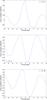 |
Fig. 9 Cross-correlation functions describing relationships between solar wind parameters (V − T, V − n, and V − B). |
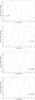 |
Fig. 10 Cross-correlation functions describing the relationship between the solar wind parameters and Dst index (V − Dst, B − Dst, BV–Dst, and BV2 − Dst). |
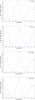 |
Fig. 11 Cross-correlation functions describing relationships between the solar wind parameters and Ap index (V–Ap, B–Ap, BV–Ap, and BV2 − Ap). |
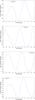 |
Fig. 12 Cross-correlation functions describing relationships between the coronal hole fractional areas CH and the solar wind parameters. |
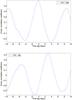 |
Fig. 13 Cross-correlation functions for CH–Dst and CH–Ap relationships. |
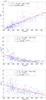 |
Fig. 14 Correlations V–T, V–n, and V–B. The linear least squares fits are shown by full lines and the power-law fits by dashed lines. The fit parameters, the correlation coefficient R, and the applied time lag Δt are shown in the insets. |
We note that the first relationship, which can be expressed as nV2 = const., resembles that of kinetic energy conservation. Similarly, the latter correlation (approximately BV = const.) resembles to the magnetic flux conservation. However, we emphasize that these relationships cannot be interpreted in this way, since there is time lag between the adopted values of V and n, as well as V and B. These empirical forms reflect a complex/dynamical time-space relationship in the solar wind, that nevertheless produce a quite simple quantitative relationship. Although their meaning is not clear, they are certainly interesting, and deserve further analysis/interpretation from the theoretical point of view.
In particular, we used the merged hourly-averaged level-2 ACE data given at http://www.srl.caltech.edu/ACE/ASC/level2/
In particular, we used the SXI coronal hole image product (level-2 files; see http://sxi.ngdc.noaa.gov/)
More details and data can be found at http://wdc.kugi.kyoto-u.ac.jp/cgi-bin/kp-cgi
Explanations and data are available at http://swdcwww.kugi.kyoto-u.ac.jp/dstdir/
Note that the unit for the product BV used in our graphs, nT × km s-1, corresponds to 0.001 mV m-1.
Acknowledgments
The research leading to the results presented in this paper has received funding from European Community’s Seventh Framework Programme (FP7/2007-2013) under grant agreement No. 218816. We are grateful to GOES-SXI and ACE teams for their open data policies. We are thankful to the referee whose constructive comments led to significant improvement of the paper.
References
- Abramenko, V., Yurchyshyn, V., & Watanabe, H. 2009, Sol. Phys., 260, 43 [NASA ADS] [CrossRef] [Google Scholar]
- Ahluwalia, H. S. 2000, J. Geophys. Res., 105, 27481 [NASA ADS] [CrossRef] [Google Scholar]
- Crooker, N. U., Feynman, J., & Gosling, J. T. 1977, J. Geophys. Res., 82, 1933 [NASA ADS] [CrossRef] [Google Scholar]
- Crowley, G., Reynolds, A., Thayer, J. P., et al. 2008, Geophys. Res. Lett., 35, 21106 [Google Scholar]
- Detman, T., Smith, Z., Dryer, M., et al. 2006, J.Geophys. Res., 111, A07102 [Google Scholar]
- Fujiki, K., Hirano, M., Kojima, M., et al. 2005, Adv. Space Res., 35, 2185 [Google Scholar]
- Gonzalez, W. D., Joselyn, J. A., Kamide, Y., et al. 1994, J. Geophys. Res., 99, 5771 [Google Scholar]
- Gopalswamy, N. 2008, J. Atmos. Solar-Terrestr. Phys., 70, 2078 [Google Scholar]
- Gopalswamy, N. 2010, in IAU Symp., 264, 326 [Google Scholar]
- Gosling, J. T. 1996, ARA&A, 34, 35 [NASA ADS] [CrossRef] [Google Scholar]
- Hill, S. M., Pizzo, V. J., Balch, C. C., et al. 2005, Sol. Phys., 226, 255 [Google Scholar]
- Kan, J. R., & Lee, L. C. 1979, Geophys. Res. Lett., 6, 577 [NASA ADS] [CrossRef] [Google Scholar]
- Krieger, A. S., Timothy, A. F., & Roelof, E. C. 1973, Sol. Phys., 29, 505 [NASA ADS] [CrossRef] [Google Scholar]
- Lee, C. O., Luhmann, J. G., Odstrcil, D., et al. 2009, Sol. Phys., 254, 155 [Google Scholar]
- Lei, J., Thayer, J. P., Forbes, J. M., Sutton, E. K., & Nerem, R. S. 2008a, Geophys. Res. Lett., 35, 10109 [Google Scholar]
- Lei, J., Thayer, J. P., Forbes, J. M., et al. 2008b, J. Geophys. Res., 113, A12, A11303 [Google Scholar]
- Lei, J., Thayer, J. P., Forbes, J. M., et al. 2008c, Geophys. Res. Lett., 35, L19105 [NASA ADS] [CrossRef] [Google Scholar]
- Luo, B., Zhong, Q., Liu, S., & Gong, J. 2008, Sol. Phys., 250, 159 [NASA ADS] [CrossRef] [Google Scholar]
- McComas, D., Bame, S. J., Barker, P., et al. 1998, Space Sci. Rev., 86, 563 [NASA ADS] [CrossRef] [Google Scholar]
- Neupert, W. M., & Pizzo, V. 1974, in BAAS, 6, 292 [Google Scholar]
- Nolte, J. T., Krieger, A. S., Timothy, A. F., et al. 1976, Sol. Phys., 46, 303 [NASA ADS] [CrossRef] [Google Scholar]
- Obridko, V. N., Shelting, B. D., Livshits, I. M., & Asgarov, A. B. 2009, Sol. Phys., 260, 191 [NASA ADS] [CrossRef] [Google Scholar]
- Odstrcil, D., & Pizzo, V. J. 2009, Sol. Phys., 250, 297 [NASA ADS] [CrossRef] [Google Scholar]
- Perreault, P., & Akasofu, S. 1978, Geophys. J. R. Astron. Soc., 54, 547 [Google Scholar]
- Pizzo, V. J., Hill, S. M., Balch, C. C., et al. 2005, Sol. Phys., 226, 283 [NASA ADS] [CrossRef] [Google Scholar]
- Richardson, I. G., & Cane, H. V. 2010, Sol. Phys., 264, 189 [NASA ADS] [CrossRef] [Google Scholar]
- Robbins, S., Henney, C. J., & Harvey, J. W. 2006, Sol. Phys., 233, 265 [Google Scholar]
- Schwenn, R. 1983, Space Sci. Rev., 34, 85 [NASA ADS] [CrossRef] [Google Scholar]
- Siscoe, G., & Crooker, N. 1974, Geophys. Res. Lett., 1, 17 [NASA ADS] [CrossRef] [Google Scholar]
- Smith, C. W., L’Heureux, J., Ness, N. F., et al. 1998, Space Sci. Rev., 86, 613 [NASA ADS] [CrossRef] [Google Scholar]
- Stone, E. C., Frandsen, A. M., Mewaldt, R. A., et al. 1998, Space Sci. Rev., 86, 1 [Google Scholar]
- Temmer, M., Vršnak, B., & Veronig, A. M. 2007, Sol. Phys., 241, 371 [NASA ADS] [CrossRef] [Google Scholar]
- Tsurutani, B. T., & Gonzalez, W. D. 1987, Planet. Space Sci., 35, 405 [NASA ADS] [CrossRef] [Google Scholar]
- Tsurutani, B. T., Gonzalez, W. D., Gonzalez, A. L. C., et al. 1995, J. Geophys. Res., 100, 21717 [Google Scholar]
- Tsurutani, B. T., Gonzalez, W. D., Guarnieri, F., et al. 2004, J. Atmos. Solar-Terrestr. Phys., 66, 167 [Google Scholar]
- Verbanac, G., Vršnak, B., Temmer, M., Mandea, M., & Korte, M. 2010, J. Atmos. Solar-Terrestr. Phys., 72, 607 [NASA ADS] [CrossRef] [Google Scholar]
- Vršnak, B., Temmer, M., & Veronig, A. 2007a, Sol. Phys., 240, 315 [Google Scholar]
- Vršnak, B., Temmer, M., & Veronig, A. 2007b, Sol. Phys., 240, 331 [Google Scholar]
All Tables
All Figures
|
Fig. 1 Time series (6-h data resolution) of CH (fractional area), T(K), n(cm-3), B(nT), V(km s-1), BV, Dst(nT), and Ap(nT), from top to bottom, respectively. The time is expressed in the day-of-year form, DOY, for 2005. |
| In the text | |
|
Fig. 2 Close-up of the interval DOY = 118−125 (HSS No. 11): a) development of Ap [nT] (bold-black) and Dst [nT] (thin-black) compared to the variation in the solar wind speed V [km s-1/10] (dashed) and the magnetic field B [nT] (bold-gray); b) Ap (bold-black) compared to the change rate of Dst (ΔDst, thin-black) and the product BV (bold-gray). |
| In the text | |
|
Fig. 3 Correlations V–Dst, B–Dst, BV − Dst,and BV2 − Dst. In panels b) − d) we separated the data points characterized by v > 450 km s-1 (circles), from those having v < 450 km s-1 (black dots). The linear least squares fit parameters, the correlation coefficient R, and the applied time lag Δt are shown in the insets; in panels b) − d) the fit parameters are shown only for the v > 450 km s-1 data (bold lines); dashed lines represent the fits for the v < 450 km s-1 data, dotted lines represent the results from Richardson & Cane (2010). |
| In the text | |
|
Fig. 4 Correlations V–Ap, B–Ap, BV–Ap, and BV2 − Ap. In panels b) − d) we separated the data points characterized by v > 450 km s-1 (circles), from those having v < 450 km s-1 (black dots). The linear least squares fit parameters, the correlation coefficient R, and the applied time lag Δt are presented in the insets; in panels b) − d), the fit parameters are for the v > 450 km s-1 data (bold line). Dashed lines are fits for the v < 450 km s-1 data; dotted lines represent an estimate of the upper limit. |
| In the text | |
|
Fig. 5 Correlation between Dst and Ap, where Dst is delayed by 0.25 days. Parameters of the linear least square fit (dashed line) are given in the inset. Bold curve represents the function |
| In the text | |
|
Fig. 6 Correlations CH–V, CH–n, CH–B, and CH–T. The linear least squares fit parameters, correlation coefficient R, and the applied time lag Δt are presented in the insets. |
| In the text | |
|
Fig. 7 Correlations CH–Dst and CH–Ap; the linear least squares fit parameters, the correlation coefficient R, and the applied time lag Δt are presented in the insets. |
| In the text | |
|
Fig. 8 a)–d) Comparison of the observed solar wind parameters with the calculated values. The observed data are inicated by the thick gray line, calculated values (using linear regression parameters a and b as given in Table 2) are drawn by thin black line, and the amplitude-optimized “predicted” values (using linear regression parameters acorr and bcorr as given in Table 2) are drawn by thick black line. e) − f) Comparison of the measured values of the geomagnetic indices Dst and Ap with the calculated values. The observed data are delineate by the thick gray line, values calculated for the N-polarity CHs are drawn by thick-dashed line, and S-polarity CHs are indicated by thick-black line. See text for details. |
| In the text | |
|
Fig. 9 Cross-correlation functions describing relationships between solar wind parameters (V − T, V − n, and V − B). |
| In the text | |
|
Fig. 10 Cross-correlation functions describing the relationship between the solar wind parameters and Dst index (V − Dst, B − Dst, BV–Dst, and BV2 − Dst). |
| In the text | |
|
Fig. 11 Cross-correlation functions describing relationships between the solar wind parameters and Ap index (V–Ap, B–Ap, BV–Ap, and BV2 − Ap). |
| In the text | |
|
Fig. 12 Cross-correlation functions describing relationships between the coronal hole fractional areas CH and the solar wind parameters. |
| In the text | |
|
Fig. 13 Cross-correlation functions for CH–Dst and CH–Ap relationships. |
| In the text | |
|
Fig. 14 Correlations V–T, V–n, and V–B. The linear least squares fits are shown by full lines and the power-law fits by dashed lines. The fit parameters, the correlation coefficient R, and the applied time lag Δt are shown in the insets. |
| In the text | |
Current usage metrics show cumulative count of Article Views (full-text article views including HTML views, PDF and ePub downloads, according to the available data) and Abstracts Views on Vision4Press platform.
Data correspond to usage on the plateform after 2015. The current usage metrics is available 48-96 hours after online publication and is updated daily on week days.
Initial download of the metrics may take a while.