| Issue |
A&A
Volume 526, February 2011
|
|
|---|---|---|
| Article Number | A20 | |
| Number of page(s) | 13 | |
| Section | The Sun | |
| DOI | https://doi.org/10.1051/0004-6361/201014617 | |
| Published online | 15 December 2010 | |
Online material
Appendix A: Cross–correlation functions
In Figs. 9 − 13, we present the cross-correlation functions between different parameters, which we used to perform the correlation scatter plots presented in the paper. All cross-correlation functions are derived up to a time lag of ±10 days, with a step of 6 h (data resolution) in all investigated cases. The time lags are always expressed in days. Negative lag between two quantities, e.g., V and Ap, hereinafter denoted as the V − Ap correlation, means that V is delayed with respect to Ap.
Appendix B: Correlation between solar-wind parameters
We calculated the cross-correlation functions for all combinations of V, T, n, and B. In Figs. 9 and 14, the cross-correlation functions and the scatter plots for the highest-correlation-coefficient time-lag are presented for the most tightly correlated combinations. All considered correlations are listed in Table 4 where the time lags Δt, the corresponding linear least squares fit parameters a and b, and the correlation coefficient R are presented. A given “X − Y” correlation corresponds to the linear form Y(t) = aX(t∗) + b, where X(t∗) represents the value of X that occurred Δt days before the actual value of Y(t), i.e., t∗ is the “retarded time”, t∗ = t − Δt.
Table 4 shows that the most tightly correlated parameters are V and T, having the correlation coefficient R = 0.8, when V is delayed after T for Δt = 0.25 days. Furthermore, Fig. 9 shows that in the V − n and V − B case, the correlation coefficients are higher when the parameters are anti-correlated (the negative correlation coefficient in Table 4). This reflects the main physical property of HSSs, which is a depleted density and magnetic field in the stream itself. The anti-correlations are most significant for the time lags Δt = 0.75 d and Δt = 2.25 d, respectively, meaning that the dips of B and n are delayed with respect to the peak of V. The positive correlations of both the V − B and V − n relationships and their negative time lags (peaks of n and B preceding the peak of V by 2.5 d and 1.75 d), are related to the magnetic field and density compression in the “interacting region” at the frontal edge of HSSs. We note that the time lag in the n − B correlation is Δt = + 0.5 d, meaning that the peak of B is delayed with respect to the peak in n.
The distribution of data points in V–n and V–B graphs in Figs. 14b and c shows two “branches”, one almost horizontal and another almost vertical. The vertical one corresponds to the slow solar wind (V ≈ 300−400 km s-1), and the horizontal one to the fast solar wind (V > 400 km s-1 and low values of n and B). If fitted by the power-law, the relationships are given by n = 1.4 × 10⁶ × V−2.0 ± 0.1, and B = 4710 × V−1.1 ± 0.1, with the correlation coefficients R = 0.69 and R = 0.58, respectively. Although the applied power-law fit is obviously more appropriate than the linear fit, it still shows a large deviation from the data in the slow-wind velocity range (v < 400 km s-1). Thus, the obtained power-law relationships can be applied only to the fast solar wind.
Relationships T(V), n(V), B(V), T(B), B(n), and T(n).
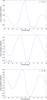 |
Fig. 9
Cross-correlation functions describing relationships between solar wind parameters (V − T, V − n, and V − B). |
| Open with DEXTER | |
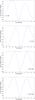 |
Fig. 10
Cross-correlation functions describing the relationship between the solar wind parameters and Dst index (V − Dst, B − Dst, BV–Dst, and BV2 − Dst). |
| Open with DEXTER | |
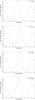 |
Fig. 11
Cross-correlation functions describing relationships between the solar wind parameters and Ap index (V–Ap, B–Ap, BV–Ap, and BV2 − Ap). |
| Open with DEXTER | |
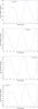 |
Fig. 12
Cross-correlation functions describing relationships between the coronal hole fractional areas CH and the solar wind parameters. |
| Open with DEXTER | |
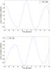 |
Fig. 13
Cross-correlation functions for CH–Dst and CH–Ap relationships. |
| Open with DEXTER | |
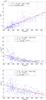 |
Fig. 14
Correlations V–T, V–n, and V–B. The linear least squares fits are shown by full lines and the power-law fits by dashed lines. The fit parameters, the correlation coefficient R, and the applied time lag Δt are shown in the insets. |
| Open with DEXTER | |
We note that the first relationship, which can be expressed as nV2 = const., resembles that of kinetic energy conservation. Similarly, the latter correlation (approximately BV = const.) resembles to the magnetic flux conservation. However, we emphasize that these relationships cannot be interpreted in this way, since there is time lag between the adopted values of V and n, as well as V and B. These empirical forms reflect a complex/dynamical time-space relationship in the solar wind, that nevertheless produce a quite simple quantitative relationship. Although their meaning is not clear, they are certainly interesting, and deserve further analysis/interpretation from the theoretical point of view.
© ESO, 2010
Current usage metrics show cumulative count of Article Views (full-text article views including HTML views, PDF and ePub downloads, according to the available data) and Abstracts Views on Vision4Press platform.
Data correspond to usage on the plateform after 2015. The current usage metrics is available 48-96 hours after online publication and is updated daily on week days.
Initial download of the metrics may take a while.