© ESO, 2011

1. Introduction

Ultra-luminous X-ray sources (ULXs) are point-like sources with luminosities greater than 10³⁹   erg   s^-1 in the 0.3−10 keV band. This high luminosity is greater than is expected from stellar mass black holes (M_BH < 20   M_⊙) accreting at the Eddington limit. Because they are usually located away from the nucleus of the galaxies, they are unlikely to be associated with super massive black holes (SMBH, M_BH > 10⁵   M_⊙), typically observed at the centre of active galactic nuclei (AGN). Their high luminosities can be explained if we assume that they host a black hole (BH) with an “intermediate mass”, around 100−10 000 M_⊙ (IMBHs, Colbert & Mushotzky 1999). However, the true nature of these sources is still unclear, and other mechanisms such as anisotropic emission (King et al. 2001) or accretion onto the BH in excess of the expected Eddington limit (Begelman 2002) could also explain them (see Roberts 2007, for a recent review). The question of what powers ULXs will be conclusively answered by a direct mass measurement based on determination of the binary orbit. However, their extragalactic nature has made the study of the ULX counterparts in other bands difficult.

In the meantime, both spectral and timing methods have been used over the past few years in an attempt to constrain the mass of the compact object in ULXs (Miller et al. 2004). A common spectral method uses the temperature and luminosity of the accretion disc emission to determine the BH mass (assuming the standard Shakura-Sunyaev models). For the timing methods, one can either use the M^cHardy et al. (2006) and Körding et al. (2007) scaling relationships of the characteristic time scales in Galactic black hole binaries (GBHs) and SMBHs with BH mass and accretion rate, or the timing-spectral scaling for the QPOs in GBHs (e.g. Shaposhnikov & Titarchuk 2007, 2009). The results from the application of this method to ULXs have been inconclusive. Some studies suggest that ULXs are stellar mass BHs (e.g. Gladstone et al. 2009; Roberts 2007; Zezas et al. 2007; Dewangan et al. 2006), while others imply that they host IMBHs (e.g. Casella et al. 2008; Miller et al. 2004).

In this paper we investigate the relationship between the X-ray variability amplitude and luminosity for a sample of 14 bright ULX sources using XMM-Newton/EPIC data. Our first aim is to measure the 2−10 keV normalised excess variance, ${\mathit{\sigma }}_{\mathrm{NXS}}^{\mathrm{2}}$, for these objects and investigate whether it correlates with the source luminosity. The normalised excess variance is a simple-to-calculate quantity that measures the intrinsic variability amplitude of a source. It can be a useful complementary tool to the full-blown power-spectrum density (PSD) analysis, and its advantage is that it can be applied to a larger number of objects as it does not require high-quality data (i.e. long, high signal-to-noise light curves).

It is well established that ${\mathit{\sigma }}_{\mathrm{NXS}}^{\mathrm{2}}$ is anti-correlated with luminosity in AGN (Nandra et al. 1997; Leighly 1999; Turner et al. 1999). Moreover, the excess variance anti-correlates with BH mass (Lu & Yu 2001; Bian & Zhao 2003; O’Neill et al. 2005; Miniutti et al. 2009; Zhou et al. 2010). Furthermore, Papadakis (2004) shows that the “variability-mass” relationship is probably the physically fundamental relationship rather than the “variability-luminosity” relationship in these objects. Our second aim is to compare the “variability-luminosity” relationship for ULXs with that of AGN with known BH mass. Following Papadakis (2004), if we assume a universal PSD shape for AGN, which scales appropriately with BH mass and accretion rate, we can then make predictions for the expected AGN “variability-luminosity” relationship at low luminosities. We want to investigate whether the ULX “variability-luminosity” data are consistent with various model “variability-luminosity” relationships for AGN, and if they are, what the implications would be for the ULX PSD shape, BH mass, and accretion rate.

In Sect. 2 we present the sample selection. In Sect. 3 we describe the data reduction, and in Sect. 4 we discuss the data analysis and present our results. We present a short discussion of their implications and our conclusions in Sects. 5 and 6, respectively.

2. The sample

We considered all bright ULXs reported in the literature, and in particular the objects studied by Heil et al. (2009) and Gladstone et al. (2009). The Heil et al. (2009) sample includes all bright ULXs that have been observed with XMM-Newton for more than 25 ks and their 0.2−10 keV flux is greater than 5 × 10^-13   erg   cm^-2   s^-1. The Gladstone et al. (2009) sample includes all ULXs observed with EPIC/XMM-Newton with more than 10 000 net counts in the 0.3−12 keV EPIC band.

One of our main aims is to compare the 2−10 keV variability amplitude of ULXs with the variability amplitude of the nearby AGN studied mainly by O’Neill et al. (2005). The length T and the bin size Δt of a light curve determine the lower and higher frequency sampled, since ν_min = 1/T and ν_max = 1/(2Δt) Hz. The excess variance of the light curve depends on the intrinsic power spectrum and also on the minimum and maximum frequencies (see Sect. 4.5). For that reason we used the same length for the light curves as those of O’Neill et al. (2005). Thus, we considered light curve segments with a length of 30−40 ks. Regarding Δt, due to the low count rate of all objects in the sample, we used bins of size 1000 s in order to increase the signal-to-noise of their light curves.

Consequently, from the Heil et al. (2009) and Gladstone et al. (2009) samples we chose those sources that were observed by XMM-Newton with a net exposure, T_net, larger than 30 ks. For this reason we did not consider the XMM-Newton data of M 33 X–8, IC 342 X−1, NGC 4395 X−1, and M 83 ULX. We did not consider NGC 4395 X−1 either because it was located on a gap of the PN detector during its XMM-Newton observation with T_net > 30 ks.

Our final sample comprises 14 ULXs. Table 1 lists their coordinates, distance, and the XMM-Newton observation details. Coordinates and distances were taken from the NASA/NED¹ database. Distances correspond to the average redshift-independent estimate for each object. For four sources (namely NGC 253 PSX-2, NGC 1313 X−1, NGC 1313 X−2, and NGC 5408 X–1) we were able to retrieve two observations from the archive with T_net larger than 30 ks. The starburst galaxy M 82 contains two ULXs, X41.4+60 and X42.3+59, which are unresolved by XMM-Newton, and they both contribute to the M 82 X−1 light curve. During the 2004 April observation that we considered in this work, approximately 84% of the observed count rate originates from X41.4+60 (Feng & Kaaret 2007).

To extend the O’Neill et al. (2005) sample to include AGN with low BH masses, we also considered the XMM-Newton observation of POX 52, which hosts an AGN with a low BH mass (M_BH = 1.6 × 10⁵   M_⊙, Barth et al. 2004). The coordinates, distance, and the XMM-Newton observation details for this source are also listed in Table 1. The distance in this case corresponds to the “luminosity distance” estimate of NASA/NED.

3. Data reduction

Data were retrieved from the XMM-Newton public data archive². We used the XMM-Newton Science Analysis System SAS³ software version 9.0.0 and followed standard procedures to extract science products from the Observation Data Files (ODFs). We used data from the EPIC-pn camera only due to its superior statistical quality. Source counts in each case were accumulated from a circular region of radius 400 pixels, centred on the source’s RA and Dec. In the case of NGC 253 PSX-2 (ObsID 152020101), we used a radius of 300 pixels to avoid contamination from a nearby source and the detector gap. Background data were extracted from a source free circular region on the same CCD chip than the source (background region radii are listed in Col. 8 of Table 1). We selected only single and double pixel events (i.e. patterns of 0−4). Bad pixels and events too close to the edges of the CCD chips were rejected using “FLAG=0.” Given the observed count rate, photon pile-up is negligible for the PN detector in all cases.

Source and background light curves in the 2−10 keV band were extracted using evselect task on SAS with a 1000-s bin. They were screened for high background (usually at the end and/or the beginning of the individual observations) and flaring activity. After rejection of the respective time intervals, the total useful observation time for each observation is usually less than the original PN exposure time. We chose to study only those light curves with at least one “clean” segment longer than 30 ks.

As an example, in the top panel of Fig. 1 we show the light curve of NGC 5408 X−1, which is typical of the light curves of all sources in the sample. The background light curve corresponds to the full PN exposure length while the source light curve is only plotted for those parts of the observation when the background activity was “low”. In general, as background “loud” we identified the observation parts where i) the background light curve showed “flare”-like events and/or prominent decreasing/increasing trends (usually at the start/end of an observation); and ii) the “net” source count rate was less than twice the background count rate. Clearly, the background light curve is stable, and of much less intensity than the “net” light curve count rate. This was the case for almost all of the light curve segments we used in this work. We also extracted the EPIC-pn spectra, after rejectioning of the time intervals affected by high background, using single and double events (PATTERN  < = 4). Response and auxiliary matrices were created with SAS tools rmfgen and arfgen, respectively.

The POX 52 XMM-Newton data were reduced in the same way. Its 2−10 keV (background subtracted) source and background light curves are also plotted in Fig. 1 (bottom panel). The observation is affected by high background flaring activity during the first  ~20 ks, and after  ~40 ks since the start of the observation, which lasted for almost 10 ks (note that this observation shows the worst background “flaring” activity among all the light curves we studied in this work).

Fig. 1 Light curves of NGC 5408 X1/ObsID 302900101 (top panel) and POX 52 (bottom panel). Stars indicate the background light curves and filled dots indicate the background-subtracted light curves, plotted only for the observation period for which the background activity is “low” (see text for details). The brackets on top of the light curves indicate the segments that were used to estimate the excess variance in each case.

4. Data analysis and results

4.1. The variability amplitude estimation

As a measure of the intrinsic variability amplitude of the light curves we computed their normalised excess variance, ${\mathit{\sigma }}_{\mathrm{NXS}}^{\mathrm{2}}$. Its square root is a measure of the average variability amplitude of a source as a fraction of the light curve mean. We used the prescription given by Vaughan et al. (2003) to estimate ${\mathit{\sigma }}_{\mathrm{NXS}}^{\mathrm{2}}$ and its error, $\mathrm{err}\mathrm{\left(}{\mathit{\sigma }}_{\mathrm{NXS}}^{\mathrm{2}}\mathrm{\right)}$⁴, as follows: ${\mathit{\sigma }}_{\mathrm{NXS}}^{\mathrm{2}}\mathrm{=}\frac{{\mathit{S}}^{\mathrm{2}}\mathrm{-}\mathrm{⟨}{\mathit{\sigma }}_{\mathrm{err}}^{\mathrm{2}}\mathrm{⟩}}{\mathrm{⟨}\mathit{x}{\mathrm{⟩}}^{\mathrm{2}}}\mathit{,}$(1)$\mathrm{err}\mathrm{\left(}{\mathit{\sigma }}_{\mathrm{NXS}}^{\mathrm{2}}\mathrm{\right)}\mathrm{=}\sqrt{\frac{\mathrm{2}}{\mathit{N}}\mathrm{(}\frac{\mathrm{⟨}{\mathit{\sigma }}_{\mathrm{err}}^{\mathrm{2}}\mathrm{⟩}}{\mathrm{⟨}\mathit{x}{\mathrm{⟩}}^{\mathrm{2}}}{\mathrm{)}}^{\mathrm{2}}\mathrm{+}\frac{\mathrm{⟨}{\mathit{\sigma }}_{\mathrm{err}}^{\mathrm{2}}\mathrm{⟩}}{\mathit{N}}\frac{\mathrm{4}{\mathit{\sigma }}_{\mathrm{NXS}}^{\mathrm{2}}}{\mathrm{⟨}\mathit{x}{\mathrm{⟩}}^{\mathrm{2}}}}\mathit{,}$(2)where x, σ_err, and N are the count rate, its error, and the number of points in the light curve, respectively and S² is the variance of the light curve, i.e.,

${\mathit{S}}^{\mathrm{2}}\mathrm{=}\frac{\mathrm{1}}{\mathit{N}\mathrm{-}\mathrm{1}}\sum _{\mathit{i}\mathrm{=}\mathrm{1}}^{\mathit{N}}\mathrm{(}{\mathit{x}}_{\mathit{i}}\mathrm{-}\mathrm{⟨}\mathit{x}\mathrm{⟩}{\mathrm{)}}^{\mathrm{2}}\mathit{.}$(3)

Following O’Neill et al. (2005), we computed ${\mathit{\sigma }}_{\mathrm{NXS}}^{\mathrm{2}}$ for each continuous light curve segment with 30 ≤ T_net ≤ 40 ks. For light curves longer than 40 ks we only considered the first 40 ks. If there were more than one segment of duration T_net longer than 30–40 ks we computed ${\mathit{\sigma }}_{\mathrm{NXS}}^{\mathrm{2}}$ for each one of them. The number of light curve segments in each observation and their T_net are listed in Table 1 (Col. 9). A few “missing” points within each segment, due to the presence of background flaring activity, appear in one of the light curve segments of NGC 4559 X−1, NGC 4945 X−2, NGC 253 PSX-2 (ObsID 152020101), and HoII X−1. Missing points are typically less than 10–15% of the total number of points. The first segment of the POX 52 light curve shows most of “missing” points (20% of the total). The presence of missing points in these segments should increase the uncertainty of the resulting ${\mathit{\sigma }}_{\mathrm{NXS}}^{\mathrm{2}}$ estimates.

Our ${\mathit{\sigma }}_{\mathrm{NXS}}^{\mathrm{2}}$ estimates for each light curve segment are listed in Table 2 (Col. 3). The numbers in parenthesis in Table 2 indicate the weighted mean ${\mathit{\sigma }}_{\mathrm{NXS}}^{\mathrm{2}}$ and its error in the case where we had more than one excess variance estimate for the same source.

The ${\mathit{\sigma }}_{\mathrm{NXS}}^{\mathrm{2}}$ measurement was negative for two sources. In these cases, we estimated the 90% upper limits of the intrinsic ${\mathit{\sigma }}_{\mathrm{NXS}}^{\mathrm{2}}$ values using the 90% upper limits on the source variance, as listed by Vaughan et al. (2003) in their Table 1. To constrain the “variability-luminosity” ULXs correlation as much as possible (see Sect. 4.3 below), we assumed a PSD slope of −1 and the upper limit from the Vaughan et al. (2003) simulations with the longest light curves (any other choice would result in an even higher 90% limit). To take the uncertainty on ${\mathit{\sigma }}_{\mathrm{NXS}}^{\mathrm{2}}$ due to the experimental Poisson fluctuations into account as well, we added the value of 1.282 err(${\mathit{\sigma }}_{\mathrm{NXS}}^{\mathrm{2}}$) to these limits. Our final estimates of the 90% confidence limits for these two sources are listed in parenthesis in Table 2.

Regarding M 82 X−1, Feng & Kaaret (2007) estimate that X41.4+60 contributes more than 80% of the observed count rate during the 2004 April XMM-Newton observation of M 82. X42.3+59 is a highly variable source, but on time scales of years (see Fig. 5 in Feng & Kaaret 2007). On shorter time scales, the same authors show that the PSD of X41.4+60 has a significantly higher amplitude than the PSD of X42.3+59.

4.2. The hard band X-ray luminosity estimation

To estimate the X-ray luminosity for each source, we fitted their spectra with an absorbed power-law model in the 2−10 keV band. For the Galactic absorption, we fixed the N_H values at the values derived from the HI maps of (Dickey & Lockman 1990). The spectral fitting was performed using XSPEC version 12.5.1. Using the best-fit results we estimated the source flux in the 2−10 keV band, hence the source luminosity, L_{2−10   keV}, adopting the distance estimates listed in Table 1. The unabsorbed L_{2−10   keV} estimates are listed in Table 2 (Col. 4)⁵. The values in parenthesis correspond to the mean L_{2−10   keV} estimates, when there were more than one spectrum for an object.

In half of the cases, the best-fit ${\mathit{\chi }}_{\mathrm{red}}^{\mathrm{2}}$ values were higher than  ~1.2. This mainly comes from the additional complexity in those spectra that the simple power-law model cannot account for (e.g. the presence of “breaks” in the high-energy spectra of these sources, Gladstone et al. 2009). Nevertheless, the power-law model adequately describes the broad shape of the source spectra in all cases, and the resulting best-fit flux measurements should accurately estimate the source X-ray continuum flux. To investigate this issue further, we used the 2−10 keV band best-fit results of Stobbart et al. (2006) to estimate the 2−10 keV luminosity for the nine sources in common. We found that L_ours = L_literature in all cases except for the NGC 55 ULX, Ho II X−1, and Ho IX X−1 sources where L_ours/L_literature = 1.1, L_ours/L_literature = 0.8, and L_ours/L_literature = 0.8, respectively. We are thus confident that our luminosity estimates are reliable. Regarding M 82 X−1, Feng & Kaaret (2007) estimate a 2−10 keV luminosity of 1.7 × 10⁴⁰ erg s^-1 for X41.4+60 during the April 2004 XMM-Newton observation of the source. This is lower than our estimate of 2.5 × 10⁴⁰ erg s^-1, but this is expected given the presence of the other ULX, which also contributes to the flux we measure from this source.

Fig. 2 Normalised excess variance versus log(L2−10   keV) for the ULXs. Arrows indicate the 90% confidence upper limits on ${\mathit{\sigma }}_{\mathrm{NXS}}^{\mathrm{2}}$ for the sources with negative excess variance estimates. The point plotted with an empty square indicates the M 82 X−1 measurement when corrected for the contribution of X42.3+59 to the observed count rate (see text for details). The shift of M 82 X−1 is shown as a dotted line. The solid line indicates the best fit to the data (excluding NGC 55 ULX).

4.3. The “variability-luminosity” relation of ULXs

Figure 2 shows ${\mathit{\sigma }}_{\mathrm{NXS}}^{\mathrm{2}}$ as function of log(L_{2−10   keV}) for the ULXs in the sample. The arrows indicate the 90% confidence upper limits on the (intrinsic) excess variance of the two sources with negative ${\mathit{\sigma }}_{\mathrm{NXS}}^{\mathrm{2}}$ estimates. The X-ray variability amplitude appears to decrease with increasing X-ray luminosity. To a large extent, this trend is driven by the NGC 55 ULX data. However, this source shows “dipping” episodes in its variability, which enhance its variability amplitude (Stobbart et al. 2004). Similar events have not been observed in other ULXs.

To investigate the significance of the apparent “variability-luminosity” relation in Fig. 2 we fitted the [log(${\mathit{\sigma }}_{\mathrm{NXS}}^{\mathrm{2}}$), log(L_{2−10   keV})] data with a straight line of the form log(${\mathit{\sigma }}_{\mathrm{NXS}}^{\mathrm{2}}\mathrm{)}\mathrm{=}\mathit{a}\mathrm{+}\mathit{b}\mathrm{\times }\log \mathrm{(}{\mathit{L}}_{\mathrm{2}\mathrm{-}\mathrm{10} \mathrm{keV}}$). Given there are oupper limits in two objects, we used the Buckley-James regression method as implemented in the software package ASURV (Isobe et al. 1986). Since the NGC 55 ULX variability properties may be somewhat “anomalous” among ULXs, we excluded this source from the fit.

The best-fit slope value is a = −1.0 ± 0.4 and is significantly different from zero at the 2.5σ level (Fig. 2). Another point in Fig. 2 indicates the M 82 X−1 measurements, when “corrected” for the contribution of X42.3+59 to the observed count rate. We have adopted the 2−10 keV luminosity measurement of Feng & Kaaret (2007) for X41.4+60. Furthermore, we increased our excess variance measurement by a factor of 1.5. This is based on the fact that “area A” and “area A+B” PSDs of Feng & Kaaret (2007) show a flat PSD at low frequencies, where the normalisation is higher by  ~1.5 for “area A” PSD. In the following figures we only indicate the “corrected” data for M 82 X−1, albeit with a different symbol than the rest of the ULX data.

4.4. Comparison with AGN

The top panel in Fig. 3 shows the “variability-luminosity” plot for the ULXs (except for the M 82 X−1 data which indicate 90% confidence upper limits), AGN using the data of O’Neill et al. (2005), data for the 4 AGN with IMBHs from Miniutti et al. (2009), and POX 52 data. The variability amplitude of this source is comparable to the amplitude of the two lowest luminosity objects in the O’Neill et al. (2005) sample and with the amplitude of the lowest luminosity object in the Miniutti et al. (2009) sample. In fact, the addition of the POX 52 and the four IMBHs data in the plot strengthens the possibility that the AGN “variability-luminosity” relation may flatten at luminosities lower than  ~10⁴²   erg   s^-1.

The solid line in the top panel of Fig. 3 indicates the best-fit line for the ULXs data while the dashed line indicates the same line shifted by Δlog (L_{2−10   keV}) = 4. The shifted line describes the AGN “variability-luminosity” relation rather well. In fact, we used the “ordinary least squares bisector” method of Isobe et al. (1990) to fit the AGN data (in the log–log space) with a straight line. The best-fit slope was −1.22 ± 0.16, which is consistent with the best-fit slope for ULXs (b_AGN − b_ULXs = 0.2 ± 0.4). Therefore, the variability amplitude may indeed decrease with increasing luminosity in a similar way for AGN and ULXs.

Despite this similarity, Fig. 3 also indicates that the ULX data are not consistent with the AGN data. For a given luminosity, even if the AGN “variability – luminosity” relation flattens below  ~10⁴²   erg   s^-1, the ULX variability amplitude is at least 10 times lower than expected when we extrapolate the AGN “variability-luminosity” relation to lower luminosities. Only NGC 55 ULX appears to be consistent with the AGN data.

4.5. Determination of model “variability-luminosity” relations

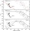Fig. 3 Normalised excess variance versus log(L2−10   keV) for ULXs (black squares, and open square for the M 82 X−1 data) and AGN (open triangles). IMBHs reported by Miniutti et al. (2009) are included as black stars and POX 52 (reported here) as an open circle. Top panel: the solid line indicates the best fit to the ULX data, and the dashed line indicates the same line shifted by +4 along the x-axis. Middle panel: the lines indicate the case A model “variability-luminosity” relation for ṁEdd = 0.03 (dotted line), 0.1 (dashed line), and 0.3 (continuous line). The short solid lines between the model curves indicate black hole masses of 5 × 106,   5 × 107, and 5 × 108   M⊙, from left to right. Bottom panel: the lines indicate the case B model “variability-luminosity” relation, for the same accretion rates. As above, the short solid lines within the model curves indicate black hole masses of 103,   104,   5 × 105,   5 × 106,   5 × 107, and 5 × 108   M⊙from left to right.

To quantitatively compare the ULXs and AGN “variability-luminosity” relationship it is necessary to derive the “excess variance – luminosity” relationship for AGN at low luminosities, and then compare it with the observed relationship for the ULXs. In this way we will be able to investigate if and for which physical parameters (i.e. M_BH, and accretion rate in units of the Eddington limit, ṁ_Edd) the ULXs data will agree with the “model” AGN “variability-luminosity” relationships.

The bolometric luminosity emitted by an AGN is ${\mathit{L}}_{\mathrm{bol}}\mathrm{=}\mathit{ṁ}{}_{\mathrm{Edd}}\mathit{L}_{\mathrm{Edd}}\mathrm{=}\mathrm{1.3}\mathit{ṁ}{}_{\mathrm{Edd}}{\mathrm{10}}^{\mathrm{38}}\mathrm{\left(}{\mathit{M}}_{\mathrm{BH}}\mathit{/}{\mathit{M}}_{\mathrm{\odot }} \mathrm{erg} {\mathrm{s}}^{-1}\mathrm{\right)}$. If k_bol is the X-ray to L_bol conversion factor, then ${\mathit{L}}_{\mathrm{2}\mathrm{-}\mathrm{10} \mathrm{keV}}\mathrm{=}{\mathit{k}}_{\mathrm{bol}}\mathrm{1.3}\mathit{ṁ}\mathrm{Edd}{\mathrm{10}}^{\mathrm{38}}\mathrm{\left(}{\mathit{M}}_{\mathrm{BH}}\mathit{/}{\mathit{M}}_{\mathrm{\odot }}\mathrm{\right)}\mathrm{erg} {\mathrm{s}}^{-1}\mathit{.}$(4)

(In all the calculations below, we adopted the k_bol − L_Edd relationship given by Lusso et al. 2010). On the other hand, the observed excess variance, estimated from a light curve of length T and bin size Δt, is an approximate measure of the integral:

${\mathit{\sigma }}_{\mathrm{NXS}}^{\mathrm{2}}\mathrm{=}{\mathrm{\int }}_{{\mathit{\nu }}_{\min }}^{{\mathit{\nu }}_{\max }}\mathit{P}\mathrm{\left(}\mathit{\nu }\mathrm{\right)}\mathrm{d}\mathit{\nu ,}$(5)

where P(ν) is the intrinsic power spectrum normalised to the square of the light curve mean, ν_min = 1/T and ν_max = 1/(2Δt). Equation (5) results from Parseval’s theorem for Fourier series and from the fact that the mean value of the periodogram (i.e. the square of the discrete Fourier transform of the light curve) is (approximately) equal to P(ν) (e.g. see discussion given in Sect. 2.2 of Vaughan et al. 2003).

The excess variance can be associated with the BH mass and accretion rate if one assumes a PSD shape and certain scaling relations between the PSD characteristic frequencies with M_BH and ṁ_Edd. Below we present model “variability-luminosity” relations for AGN, assuming two rather simple scenarios for their PSD shapes, which are based on recent power spectral studies of AGN and GBHs.

Case A: Analyses based on high-quality RXTE and XMM-Newton light curves have shown that the AGN PSDs can be approximated by a broken power law, with P(ν) = A(ν/ν_br)^-1 and P(ν) = A(ν/ν_br)^-2 at frequencies below and above a characteristic frequency break, ν_br (e.g. Markowitz et al. 2003; M^cHardy et al. 2004). M^cHardy et al. (2006) demonstrate that ν_br depends on both M_BH and ṁ_Edd as

$\begin{array}{ccc}{\mathit{\nu }}_{\mathrm{br}}\mathrm{=}\mathrm{0.003}\mathit{ṁ}\mathrm{Edd}\mathrm{(}{\mathit{M}}_{\mathrm{BH}}\mathit{/}{\mathrm{10}}^{\mathrm{6}} {\mathit{M}}_{\mathrm{\odot }}{\mathrm{)}}^{-1}\mathit{.}& & \end{array}$(6)

In this case (case A model hereafter), it is straightforward to show that

$\begin{array}{ccc}{\mathit{\sigma }}_{\mathrm{NXS}}^{\mathrm{2}}\mathrm{=}\{\begin{array}{c}\\ & \\ & \\ & \end{array}& & \end{array}$(7)

where C₁ = Aν_br. Following Papadakis (2004) we assumed that C₁ = 0.02. The solid line in Fig. 4 indicates the case A PSD model, when ν_br = 10^-3 and A = 20 Hz^-1 (values chosen arbitrarily). The area below the case A PSD curve, and between ν_min and ν_max values, according to Eq. (5) should be (approximately) equal to ${\mathit{\sigma }}_{\mathrm{NXS}}^{\mathrm{2}}$.

Fig. 4 The assumed PSD shape in case A (continuous line) and case B (dashed line) scenarios discussed in Sect. 4.5. νbr and νbr,2 are the characteristic “frequency breaks”, at which the PSD slope changes, while νmin and νmax are the minimum and maximum frequencies sampled by the light curve segments used in this work. We assume a second break frequency which is 10 times smaller than νbr. The regions filled with diagonal-dotted lines (vertical-continuous lines) indicate the area below the PSD shape in case A (case B) scenario which should be approximately equal to the excess variance of the light curves. This area (hence ${\mathit{\sigma }}_{\mathrm{NXS}}^{\mathrm{2}}$ as well) depends on the location of the break frequencies (determined by black hole mass and accretion rate) with respect to νmax and νmin (which are fixed according to the values T and Δt of the light curves used in this work).

Case B: A second frequency break, ν_br,2, below which the PSD is roughly flat (i.e. P(ν) ∝ ν⁰), has also been observed in at least one AGN (i.e. Ark 564, Papadakis et al. 2002; M^cHardy et al. 2007) and in GBHs in “low/hard” and “very high” states (see discussion in Sect. 5.1 below). The PSDs in the latter case are quite complex, usually described by a series of Lorentzians (e.g. Pottschmidt et al. 2003). However, the entire spectral shape roughly resembles a (doubly) broken power law of the form: P(ν) = A(ν/ν_br)^-2, for ν > ν_br, P(ν) = A(ν/ν_br)^-1, for ν_br,2 < ν < nu_br and P(ν) = A(ν_br,2/ν_br)^-1 = const., for ν < ν_br,2. In this case (case B model hereafter), the excess variance of the light curves should be ${\mathit{\sigma }}_{\mathrm{NXS}}^{\mathrm{2}}\mathrm{=}\{\begin{array}{c}\\ {\mathit{C}}_{\mathrm{1}}{\mathit{\nu }}_{\mathrm{br}}\mathrm{(}{\mathit{\nu }}_{\min }^{-1}\mathrm{-}{\mathit{\nu }}_{\max }^{-1}\mathrm{)}\mathit{,}& \mathrm{(}\mathrm{if} {\mathit{\nu }}_{\mathrm{br}\mathit{,}\mathrm{2}}\mathit{,}{\mathit{\nu }}_{\mathrm{br}}\mathit{<}{\mathit{\nu }}_{\min }\mathrm{)}& \\ {\mathit{C}}_{\mathrm{1}}\mathrm{\left[}\ln \mathrm{\right(}\frac{{\mathit{\nu }}_{\mathrm{br}}}{{\mathit{\nu }}_{\min }}\mathrm{)}\mathrm{-}\frac{{\mathit{\nu }}_{\mathrm{br}}}{{\mathit{\nu }}_{\max }}\mathrm{+}\mathrm{1}\mathrm{]}\mathit{,}& \mathrm{(}\mathrm{if} {\mathit{\nu }}_{\min }\mathit{<}{\mathit{\nu }}_{\mathrm{br}}\mathit{<}{\mathit{\nu }}_{\max } \mathrm{and} {\mathit{\nu }}_{\mathrm{br}\mathit{,}\mathrm{2}}\mathit{<}{\mathit{\nu }}_{\min }\mathrm{)}& \\ {\mathit{C}}_{\mathrm{1}}\ln \mathrm{\left(}\frac{{\mathit{\nu }}_{\max }}{{\mathit{\nu }}_{\min }}\mathrm{\right)}\mathit{,}& \mathrm{(}\mathrm{if} {\mathit{\nu }}_{\mathrm{br}}\mathit{>}{\mathit{\nu }}_{\max } \mathrm{and} {\mathit{\nu }}_{\mathrm{br}\mathit{,}\mathrm{2}}\mathit{<}{\mathit{\nu }}_{\min }\mathrm{)}& \\ {\mathit{C}}_{\mathrm{1}}\mathrm{\left[}\ln \mathrm{\right(}\frac{{\mathit{\nu }}_{\mathrm{br}}}{{\mathit{\nu }}_{\mathrm{br}\mathit{,}\mathrm{2}}}\mathrm{)}\mathrm{+}\mathrm{2}\mathrm{-}\frac{{\mathit{\nu }}_{\min }}{{\mathit{\nu }}_{\mathrm{br}\mathit{,}\mathrm{2}}}\mathrm{-}\frac{{\mathit{\nu }}_{\mathrm{br}}}{{\mathit{\nu }}_{\max }}\mathrm{]}\mathit{,}& \mathrm{\left(}\mathrm{if} {\mathit{\nu }}_{\min }\mathit{<}{\mathit{\nu }}_{\mathrm{br}\mathit{,}\mathrm{2}}\mathit{<}{\mathit{\nu }}_{\mathrm{br}}\mathit{<}{\mathit{\nu }}_{\max }\mathrm{\right)}& \\ {\mathit{C}}_{\mathrm{1}}\mathrm{\left[}\ln \mathrm{\right(}\frac{{\mathit{\nu }}_{\max }}{{\mathit{\nu }}_{\mathrm{br}\mathit{,}\mathrm{2}}}\mathrm{)}\mathrm{+}\mathrm{1}\mathrm{-}\frac{{\mathit{\nu }}_{\min }}{{\mathit{\nu }}_{\mathrm{br}\mathit{,}\mathrm{2}}}\mathrm{]}\mathit{,}& \mathrm{\left(}\mathrm{if} {\mathit{\nu }}_{\min }\mathit{<}{\mathit{\nu }}_{\mathrm{br}\mathit{,}\mathrm{2}}\mathit{<}{\mathit{\nu }}_{\max } \mathrm{and} {\mathit{\nu }}_{\mathrm{br}}\mathit{>}{\mathit{\nu }}_{\max }\mathrm{\right)}& \\ {\mathit{C}}_{\mathrm{1}}\mathrm{(}{\mathit{\nu }}_{\max }\mathrm{-}{\mathit{\nu }}_{\min }\mathrm{)}\mathit{/}{\mathit{\nu }}_{\mathrm{br}\mathit{,}\mathrm{2}}\mathit{,}& \mathrm{\left(}\mathrm{if} {\mathit{\nu }}_{\mathrm{br}\mathit{,}\mathrm{2}}\mathit{,} {\mathit{\nu }}_{\mathrm{br}}\mathit{>}{\mathit{\nu }}_{\max }\mathrm{\right)}\mathit{.}& \end{array}$(8)

The ratio ν_br/ν_br,2 is usually  ~10 in GBHs. We adopted the Axelsson et al. (2006) relation between the two break frequencies in Cyg X−1⁶:

${\mathit{\nu }}_{\mathrm{br}\mathit{,}\mathrm{2}}\mathrm{=}\mathrm{0.15}{\mathit{\nu }}_{\mathrm{br}}^{\mathrm{1.2}}\mathit{.}$(9)

The area below the the case B PSD curve between ν_min and ν_max is approximately equal to ${\mathit{\sigma }}_{\mathrm{NXS}}^{\mathrm{2}}$. We can now use the equations above to construct AGN model “variability-luminosity” relations as follows.

4.6. The AGN model “variability-luminosity” relations

We considered BH mass values in the range 10³−10⁹   M_⊙, and three accretion rate values, namely 0.03, 0.1 and 0.3 of the Eddington limit. For any given M_BH and ṁ_Edd values, we used Eq. (4) to compute the 2−10 keV luminosity of the source, and Eqs. (6) and (9) to compute ν_br and ν_br,2, respectively. We then used Eqs. (7) and (8) to compute the model ${\mathit{\sigma }}_{\mathrm{NXS}}^{\mathrm{2}}$ values in case A and case B scenarios, respectively. The minimum and maximum sampled frequencies in our case are ν_max = 1/(2 × 1000) Hz and ν_min = 1/T_mean Hz, where T_mean = 37 ks, i.e. the average length of all the segments listed in Col. (9) of Table  1. The resulting model “variability-luminosity” relations are plotted in Fig. 3 (middle and bottom panels).

The agreement between the expected case A “variability-luminosity” relations for ṁ_Edd = 0.03, 0.1, and 0.3 (see Fig. 3, middle panel) and the AGN data is reasonably good, indicating that both the shape and the scatter in the observed “variability-luminosity” relation for AGN can be explained if the nearby, bright type-1 Seyferts accrete at  ~3−30% of the Eddington limit. The flattening of the relation at low luminosities results when Eq. (6) is valid, then ν_br > ν_max for objects with BH mass (luminosity) less than  ~2−6 × 10⁵   M_⊙ [(0.6−4.0) × 10⁴¹   erg   s^-1]. Consequently, the excess variance should remain constant (see bottom relationship in the set of Eqs. (7)) for all objects with lower M_BH (and therefore source luminosity).

The bottom panel of Fig. 3 indicate the case B “variability-luminosity” predictions (as before, we considered the values of ṁ_Edd = 0.03, 0.1, and 0.3). If there is indeed a second PSD frequency break, and Eqs. (6) and (9) are valid, then we expect ν_br,2 > ν_min for sources with BH mass (luminosity) less than  ~6 × 10⁵   M_⊙ (~4 × 10⁴¹   erg   s^-1). Since the low-frequency flat part of the PSD does not contribute to the integral defined by Eq. (1) as much as the ν^-1 part does (see Fig. 4), the excess variance is expected to decrease with decreasing luminosity when L_{2−10   keV} < 4 × 10⁴¹   erg   s^-1.

Fig. 5 Normalised excess variance versus log(L2−10   keV) for the ULXs. The dotted-filled region indicates the area with BH mass of (2.5−30) × 103   M⊙ and accretion rates of ṁEdd = (0.01−0.8). Dashed lines indicate the case B model for AGN-like objects with a BH mass of (2.5−30) × 103   M⊙ (from left to right along each line), and for accretion rates of ṁEdd =  [0.01, 0.05, 0.1, 0.2, 0.5, 0.8] (from top to bottom).

4.7. The comparison between ULXs and AGN revisited

It is clear from the middle panel of Fig. 3 that, apart from NGC 55 ULX, the ULXs data are not consistent with the case A AGN model predictions. On the other hand, the bottom panel in Fig. 3 shows that most of the ULXs data are consistent with the case B model “variability-luminosity” relations.

In Fig. 5 we again plot the ${\mathit{\sigma }}_{\mathrm{NXS}}^{\mathrm{2}}\mathrm{-}\log \mathrm{\left(}{\mathit{L}}_{\mathrm{2}\mathrm{-}\mathrm{10} \mathrm{keV}}\mathrm{\right)}$ data for the ULXs. The fact that most of the ULXs data are located within the boundaries of the diagonally dashed region of the plot implies that these objects may operate like AGN, with a BH mass in the range (2.5−30) × 10³   M_⊙, and an accretion rate in the range  [0.01−0.8] . Regarding NGC 2403 X−1 and NGC 4945 X−2 (the upper limits), their low variability amplitude can be explained if they host a BH with a mass close to or even lower than 2.5 × 10³   M_⊙.

Furthermore, the same figure can also explain the apparent ULX “variability-luminosity” anti-correlation. If the higher-luminosity objects in the sample have systematically larger BH  mass and accretion rate than the lower-luminosity objects, then their variability amplitude should also be systematically smaller, hence the “smaller variability amplitude with increasing luminosity” trend we detected.

Finally, it is clear from Fig. 3 that NGC 55 ULX is not consistent with the case B model predictions. One could assume that this source is more consistent with the case A model predictions; however, the high amplitude dipping episodes seen in the light curve of this source are not commonly seen in AGN light curves. Furthermore, if that were the case, we would expect that ν_br > ν_max for this object and that its PSD has a −1 slope in the frequency range  ~10^-4−10^-3 Hz. However, Heil et al. (2009) find an average PSD slope of −1.96 ± 0.04 in this frequency range. Therefore, the agreement of the NGC 55 ULX data with the case A “excess variance-luminosity” relation must be coincidental.

5. Discussion

We present the results of a variability analysis of a sample of 14 bright ULXs using 19 observations with XMM-Newton/EPIC. We calculated their normalised excess variance using light curves of 40 ks length. Our main aim was to compare their “variability-luminosity” relationship with the same relationship for AGN. Our main results can be summarised as

• the variability amplitude of ULXs is significantly smaller thanexpected from a simple extrapolation of the AGN“variability-luminosity” relationship to lower luminosities;

• we found evidence that the variability amplitude in ULXs decreases with increasing 2−10 keV source luminosity. This “variability-luminosity” anti-correlation is similar (in slope) to what is observed in nearby type 1 Seyferts.

We discuss in some detail some implications of our results below.

5.1. Are most ULXs AGN-like objects?

This ULXs show a significantly smaller variability amplitude (when compared to the amplitude expected from an extrapolation of the AGN “variability-luminosity” relation to low luminosities) is consistent with the hypothesis that ULXs are “scaled-down” versions of the nearby AGN, but only if a) there two break frequencies in their PSDs, b) ν_br scales with BH mass and accretion rate as in Eq. (6), c) ν_br/ν_br,2 ~ 5−50, and d) ν_br,2 (i.e. the frequency where the PSD shape changes from a slope of 0 to  ~−1) is higher than 3 × 10^-5 Hz.

This band-limited noise PSD shape is commonly observed in GBHs in their “low/hard" and “very high” states (VHS; see for example Figs. 4e and c in Klein-Wolt & van der Klis 2008). In this case the variability is mostly limited to  ~1−2 decades of temporal frequency. In most AGN though, the PSDs resemble the GBHs in their “high state”, because the 1/ν part of the power spectrum extends over many decades of frequency below ν_br (M^cHardy et al. 2006). The only exception is Ark 564, where a second PSD break (to a slope flatter than −1) is observed, and most of the variability is indeed limited in less than two decades of frequency. Interestingly, Ark 564 is the only high accretion rate AGN for which a good quality PSD is available at the moment. M^cHardy et al. (2007) suggest that this object is the AGN analogue of GBHs in VHS. Perhaps then, just like Ark 564, ULXs are also similar to GBHs in VHS.

Are there any indications that ULXs power spectra have a shape consistent with the PSD model outlined above? Recently, Heil et al. (2009) has presented the results from a detailed PSD analysis of archival ULX light curves. They detected “0 to –1” PSD breaks at frequencies higher than 3 × 10^-5 Hz in NGC 5408 X−1 and M 82 X−1. In NGC 1313 X−1 they detected a “0 to –2” break, however the best-fit high-frequency slope has a large uncertainty (−2.35 ± 1). The possibility of a –1 slope cannot be excluded, as it is just 1.35σ away from the best-fit value. The “0 to –2” PSD slope breaks are unusual in GBHs.

On the other hand, the same authors find that the PSD of Ho IX X−1, NGC 1313 X−2, and NGC 55 ULX were best-fitted by a simple power-law model. The −2 PSD slope in NGC 55 ULX is not consistent with the case A or case B scenarios either (see also Sect. 4.7). The best-fit slope for NGC 1313 X−2 is also steep (~−2), but it is based on just one point (see e.g. the top left panel in Fig. 1 of Heil et al. 2009), while the best-fit slope of Ho IX X−1 is flat, close to  ~−0.5. This may indicate of a ν_br,2 break just below the lowest frequency of 10^-4 Hz that Heil et al. (2009) considered. We therefore believe that the results of Heil et al. (2009) do agree with the case B PSD shape we outlined in the previous section.

5.2. Constrains on the BH mass and accretion rate of ULXs

If most of the ULXs in the sample indeed operate like AGN and their PSDs are consistent with the case B scenario outlined in Sect. 4.5, then they must host a black hole with a mass of M_BH ~ 2500−3 × 10⁴ M_⊙, which accretes at  ~1−80% of the Eddington limit. Lower BH masses with a higher accretion rate or higher BH masses with a lower accretion rate cannot be consistent with most of the ULX data shown in Fig. 3. To illustrate this point, we notice the line for 10³   M_⊙ in the bottom panel of Fig. 3, which indicates the expected $\mathrm{\left[}{\mathit{\sigma }}_{\mathrm{rms}}^{\mathrm{2}}\mathit{,}\log \mathrm{(}{\mathit{L}}_{\mathrm{2}\mathrm{-}\mathrm{10} \mathrm{keV}}\mathrm{\right)}\mathrm{]}$ relationship in the case B model for objects with M_BH = 10³M_⊙ and $\mathrm{0.03}\mathit{<}\mathit{ṁ}{\mathrm{Edd}}_{}\mathit{<}\mathrm{0.3}$. Clearly, this line is inconsistent with the ULX data. An increase of k_bol by a factor of  ~10 would be required shifting this line along the x-axis by the same factor, hence to be roughly consistent with the ULX data. This difference in k_bol would imply a significant difference between the ULX and AGN spectral energy distributions. Thus, if most of the ULXs in our sample indeed host a BH mass that is significantly lower than (1−10) × 10³   M_⊙, then they are not exactly like AGN.

Wu & Gu (2008) also address the questions “do ULXs operate like-AGN?”, and, “if yes, what should their BH mass be”? They studied the relationship between Γ and X-ray luminosity in seven ULXs (four of them included in our sample). They find that it is similar to what is observed in GBHs and AGN and that the ULX central BH mass should be  ~10⁴   M_⊙, in agreement with our results. Strohmayer & Mushotzky (2009) show that the pattern of spectral and temporal correlations in NGC 5408 X–1 is analogous to what is seen in GBHs,and argue that the BH mass range for this system is from (2−9) × 10³   M_⊙. The position of the NGC 5408 X−1 data in Fig. 2 is consistent with an object with a BH mass of  ~6 × 10³   M_⊙ which accretes at  ~4% of the Eddington limit, in agreement with the BH mass range of Strohmayer & Mushotzky (2009). As for the M 82 X−1 data in the same figure, they suggested a BH mass of 1.8 × 10⁴   M_⊙ in the system. This is 2−3 times larger than the most likely BH mass range of “one to a few thousand solar masses” for this source, as estimated by Kaaret et al. (2009). This is not a significant discrepancy, because we would need many observations to estimate the average variability amplitude and X-ray luminosity of the source to compare it with the models, and therefore accurately predict the BH mass and accretion rate for an individual object.

5.3. Do all ULXs in our sample operate in the “same” way?

Obviously, NGC 55 ULX does not operate in the same way as the other objects in the sample. Its large variability amplitude can be explained with neither the case A nor the case B possibilities. This is not surprising, given the “dipping” episodes that have been observed in its light curve, and not in other ULXs (or AGN). Due to the presence of these “dips”, the source light curves have a large variability amplitude for its luminosity.

Heil et al. (2009) notice that the strength of the intrinsic variability in ULXs like NGC 4559 X−1, NGC 5204 X−1, and Ho II X−1 is substantially lower than the observed variability amplitude seen in other sources. These objects are also included in our sample, but we found that their excess variance (i.e. their X-ray variability amplitude) is consistent with the one observed in the other ULXs. It could be due to the technical difficulty of the estimation of the PSD fit for faint sources like ULXs. On the other hand, we found that ${\mathit{\sigma }}_{\mathrm{NXS}}^{\mathrm{2}}$ is not constrained in two other ULXs, namely NGC 4945 X−2 and NGC 2403 X−1. Given the large error on the ${\mathit{\sigma }}_{\mathrm{NXS}}^{\mathrm{2}}$ measurement for these two objects, it is not clear whether their intrinsic variability amplitude is indeed “significantly smaller” than the amplitude of the other sources. In any case, if the BH mass and accretion rate of the objects in the sample are in the range of (2.5−30) × 10³   M_⊙ and  ~1−80%, we do expect their intrinsic excess variance to differ by a factor of  ~100 (see Fig. 5). In other words, significant differences among the variability amplitude of ULXs do not necessarily imply that there are any fundamental differences in their emission mechanism, but they could be due to differences in their BH mass and/or accretion rate.

5.4. The “variability-luminosity” anti-correlation in ULXs

We found evidence for an anti-correlation between the variability amplitude and the X-ray luminosity of the ULXs we studied. We estimated the significance of this correlation at the 2.5σ level. To the best of our knowledge, this is the first time that a “variability-luminosity” anti-correlation has been detected in ULXs. A similar anti-correlation has also been pointed out by Heil et al. (2009) (see right panel in their Fig. 4). They parametrised the variability amplitude by means of the power-spectrum amplitude at a given frequency, which is significantly more difficult to measure than the excess variance. As a result, they could measure only upper limits on the variability amplitude of many sources. Consequently, when excluding the NGC 55 ULX data and the points with upper limits, the significance of the “variability-luminosity” anti-correlation was substantially decreased.

The similarity between the slope of the “variability-luminosity” relationship for AGN and ULXs argues in favour of the reliability of this anti-correlation in ULXs. However, the amplitude of these two relationships is significantly different. Under the case B scenario discussed above, this anti-correlation could be explained if the high-luminosity objects in the sample have higher BH masses and a higher accretion rate. In this case they should also have smaller variability amplitudes, as observed.

However, there are reasons for which the correlation shown in Fig. 2 may be misleading. Firstly, the luminosity of the sources in the sample covers a rather limited range of values between (2.5−30) × 10³⁹   erg   s^-1. In this case, even a small error in the luminosity estimation (due to an inaccurate distance and/or flux measurement for example) may shift the position of data points in this plot, and hence affect our results. We performed a numerical experiment to investigate this effect. We used the present $\mathrm{(}{\mathit{\sigma }}_{\mathrm{NXS}}^{\mathrm{2}}\mathrm{-}{\mathit{L}}_{\mathrm{2}\mathrm{-}\mathrm{10} \mathrm{keV}}\mathrm{)}$ data set (excluding NGC 55 ULX) to create 100 new sets. In each run, we randomly decreased and/or increased the luminosity of all points by a factor of 2. We then fitted the new data set (in the log-log space) using ASURV (to take the upper limits into account on the data points with negative excess variance measurements, exactly as we did with the real data points) and recorded the best-fit slope value. In all cases, the best-ft slope was different from zero at the (2.2−2.5)σ level. The results from this experiment indicate that, most probably, “luminosity-induced” uncertainties cannot seriously affect the observed anti-correlation.

However, the most “serious” reason against the reliability of this anti-correlation is the small size of our sample. A larger number of ULXs would be necessary to confirm it. Furthermore, a conclusive test of the “variability-amplitude” anti-correlation in ULXs will be possible when future observations of ULXs will allow us to determine their average excess variance and average X-ray luminosity, and examine whether they are anti-correlated. If this correlation is confirmed, it would indicate that ULXs show a fundamental physical link between BH mass (i.e. luminosity) and accretion rate. If this correlation is not confirmed, then what we observe in this work can only be a coincidence due to incompleteness of the sample.

6. Conclusions

The main result of this work is that the variability amplitude of ULXs is significantly smaller than the amplitude predicted by a simple extrapolation to low luminosities of the well established “variability-amplitude” relationship for the nearby bright AGN. This discrepancy can be consistent with the hypothesis that most ULXs operate like AGN, but only if (i) they host an IMBH of  ~(2.5−30) × 10³   M_⊙; (ii) their accretion rate is 1−80%

of the Eddington limit; and (iii) their PSDs have the band-limited noise shape shown by GBHs in their “low-hard” and “very-high” state.

We also found evidence of an anti-correlation between the normalised excess variance and the luminosity for ULXs. The slope is consistent with the one found in AGN but with an offset in luminosity of around four orders of magnitudes. A larger sample of ULXs and determination of their average X-ray luminosity and variability amplitude, is needed to confirm its significance.

Acknowledgments

We thank the referee for helpful comments and suggestions. We acknowledge support by the EU FP7-REGPOT 206469 and ToK 39965 grants. This work is based on observations with XMM-Newton, an ESA science mission with instruments and contributions directly funded by ESA Member States and the USA (NASA).

References

All Tables

All Figures

Fig. 1 Light curves of NGC 5408 X1/ObsID 302900101 (top panel) and POX 52 (bottom panel). Stars indicate the background light curves and filled dots indicate the background-subtracted light curves, plotted only for the observation period for which the background activity is “low” (see text for details). The brackets on top of the light curves indicate the segments that were used to estimate the excess variance in each case.

In the text

Fig. 2 Normalised excess variance versus log(L2−10   keV) for the ULXs. Arrows indicate the 90% confidence upper limits on ${\mathit{\sigma }}_{\mathrm{NXS}}^{\mathrm{2}}$ for the sources with negative excess variance estimates. The point plotted with an empty square indicates the M 82 X−1 measurement when corrected for the contribution of X42.3+59 to the observed count rate (see text for details). The shift of M 82 X−1 is shown as a dotted line. The solid line indicates the best fit to the data (excluding NGC 55 ULX).

In the text

Fig. 3 Normalised excess variance versus log(L2−10   keV) for ULXs (black squares, and open square for the M 82 X−1 data) and AGN (open triangles). IMBHs reported by Miniutti et al. (2009) are included as black stars and POX 52 (reported here) as an open circle. Top panel: the solid line indicates the best fit to the ULX data, and the dashed line indicates the same line shifted by +4 along the x-axis. Middle panel: the lines indicate the case A model “variability-luminosity” relation for ṁEdd = 0.03 (dotted line), 0.1 (dashed line), and 0.3 (continuous line). The short solid lines between the model curves indicate black hole masses of 5 × 106,   5 × 107, and 5 × 108   M⊙, from left to right. Bottom panel: the lines indicate the case B model “variability-luminosity” relation, for the same accretion rates. As above, the short solid lines within the model curves indicate black hole masses of 103,   104,   5 × 105,   5 × 106,   5 × 107, and 5 × 108   M⊙from left to right.

In the text

Fig. 4 The assumed PSD shape in case A (continuous line) and case B (dashed line) scenarios discussed in Sect. 4.5. νbr and νbr,2 are the characteristic “frequency breaks”, at which the PSD slope changes, while νmin and νmax are the minimum and maximum frequencies sampled by the light curve segments used in this work. We assume a second break frequency which is 10 times smaller than νbr. The regions filled with diagonal-dotted lines (vertical-continuous lines) indicate the area below the PSD shape in case A (case B) scenario which should be approximately equal to the excess variance of the light curves. This area (hence ${\mathit{\sigma }}_{\mathrm{NXS}}^{\mathrm{2}}$ as well) depends on the location of the break frequencies (determined by black hole mass and accretion rate) with respect to νmax and νmin (which are fixed according to the values T and Δt of the light curves used in this work).

In the text

Fig. 5 Normalised excess variance versus log(L2−10   keV) for the ULXs. The dotted-filled region indicates the area with BH mass of (2.5−30) × 103   M⊙ and accretion rates of ṁEdd = (0.01−0.8). Dashed lines indicate the case B model for AGN-like objects with a BH mass of (2.5−30) × 103   M⊙ (from left to right along each line), and for accretion rates of ṁEdd =  [0.01, 0.05, 0.1, 0.2, 0.5, 0.8] (from top to bottom).

In the text

References

- Axelsson, M., Borgonovo, L., & Larsson, S. 2006, A&A, 452, 975 [NASA ADS] [CrossRef] [EDP Sciences] [Google Scholar]
- Barth, A. J., Ho, L. C., Rutledge, R. E., & Sargent, W. L. W. 2004, ApJ, 607, 90 [NASA ADS] [CrossRef] [Google Scholar]
- Barnard, R. 2010, MNRAS, 231 [Google Scholar]
- Begelman, M. C. 2002, ApJ, 568, L97 [NASA ADS] [CrossRef] [Google Scholar]
- Bian, W., & Zhao, Y. 2003, ApJ, 591, 733 [NASA ADS] [CrossRef] [Google Scholar]
- Casella, P., Ponti, G., Patruno, A., et al. 2008, MNRAS, 387, 1707 [NASA ADS] [CrossRef] [Google Scholar]
- Dewangan, G. C., Titarchuk, L., & Griffiths, R. E. 2006, ApJ, 637, L21 [NASA ADS] [CrossRef] [Google Scholar]
- Colbert, E. J. M., & Mushotzky, R. F. 1999, ApJ, 519, 89 [NASA ADS] [CrossRef] [Google Scholar]
- Dewangan, G. C., Mathur, S., Griffiths, R. E., & Rao, A. R. 2008, ApJ, 689, 762 [NASA ADS] [CrossRef] [Google Scholar]
- Dickey, J. M., & Lockman, F. J. 1990, ARA&A, 28, 215 [NASA ADS] [CrossRef] [MathSciNet] [Google Scholar]
- Feng, H., & Kaaret, P. 2007, ApJ, 668, 941 [NASA ADS] [CrossRef] [Google Scholar]
- Gladstone, J. C., Roberts, T. P., & Done, C. 2009, MNRAS, 397, 1836 [NASA ADS] [CrossRef] [Google Scholar]
- Heil, L. M., Vaughan, S., & Roberts, T. P. 2009, MNRAS, 397, 1061 [NASA ADS] [CrossRef] [Google Scholar]
- Isobe, T., Feigelson, E. D., & Nelson, P. I. 1986, ApJ, 306, 490 [NASA ADS] [CrossRef] [Google Scholar]
- Isobe, T., Feigelson, E. D., Akritas, M. G., & Babu, G. J. 1990, ApJ, 364, 104 [NASA ADS] [CrossRef] [EDP Sciences] [Google Scholar]
- Kaaret, P., Prestwich, A. H., Zezas, A., et al. 2001, MNRAS, 321, L29 [Google Scholar]
- Kaaret, P., Feng, H., & Gorski, M. 2009, ApJ, 692, 653 [NASA ADS] [CrossRef] [Google Scholar]
- King, A. R., Davies, M. B., Ward, M. J., Fabbiano, G., & Elvis, M. 2001, ApJ, 552, L109 [NASA ADS] [CrossRef] [Google Scholar]
- Klein-Wolt, M., & van der Klis, M. 2008, ApJ, 675, 1407 [NASA ADS] [CrossRef] [Google Scholar]
- Körding, E. G., Migliari, S., Fender, R., et al. 2007, MNRAS, 380, 301 [NASA ADS] [CrossRef] [Google Scholar]
- Leighly, K. M. 1999, ApJS, 125, 317 [NASA ADS] [CrossRef] [Google Scholar]
- Lu, Y., & Yu, Q. 2001, ApJ, 561, 660 [NASA ADS] [CrossRef] [Google Scholar]
- Lusso, E., Comastri, A., Vignali, C., et al. 2010, A&A, 512, A34 [NASA ADS] [CrossRef] [EDP Sciences] [Google Scholar]
- Markowitz, A., Edelson, R., Vaughan, J., et al. 2003, ApJ, 593, 96 [NASA ADS] [CrossRef] [Google Scholar]
- Martocchia, A., Matt, G., Belloni, T., et al. 2006, A&A, 448, 677 [NASA ADS] [CrossRef] [EDP Sciences] [Google Scholar]
- Matsumoto, H., Tsuru, T. G., Koyama, K., et al. 2001, ApJ, 547, L25 [NASA ADS] [CrossRef] [Google Scholar]
- Mc Hardy, I. M., Papadakis, I. E., Uttley, P., et al. 2004, MNRAS, 348, 783 [NASA ADS] [CrossRef] [Google Scholar]
- Mc Hardy, I. M., Koerding, E., Knigge, C., Uttley, P., & Fender, R. P. 2006, Nature, 444, 730 [NASA ADS] [CrossRef] [PubMed] [Google Scholar]
- Mc Hardy, I. M., Arévalo, P., Uttley, P., et al. 2007, MNRAS, 382, 985 [NASA ADS] [CrossRef] [Google Scholar]
- Miller, J. M., Fabian, A. C., & Miller, M. C. 2004, ApJ, 614, L117 [NASA ADS] [CrossRef] [Google Scholar]
- Miniutti, G., Ponti, G., Greene, J. E., et al. 2009, MNRAS, 394, 443 [NASA ADS] [CrossRef] [Google Scholar]
- Nandra, K., George, I. M., Mushotzky, R. F., Turner, T. J., & Yaqoob, T. 1997, ApJ, 476, 70 [NASA ADS] [CrossRef] [Google Scholar]
- O’Neill, P. M., Nandra, K., Papadakis, I. E., & Turner, T. J. 2005, MNRAS, 358, 1405 [NASA ADS] [CrossRef] [Google Scholar]
- Papadakis, I. E. 2004, MNRAS, 348, 207 [NASA ADS] [CrossRef] [Google Scholar]
- Papadakis, I. E., Brinkmann, W., Negoro, H., & Gliozzi, M. 2002, A&A, 382, L1 [NASA ADS] [CrossRef] [EDP Sciences] [Google Scholar]
- Pottschmidt, K., Wilms, J., Nowak, M. A., et al. 2003, A&A, 407, 1039 [NASA ADS] [CrossRef] [EDP Sciences] [Google Scholar]
- Roberts, T. P. 2007, Ap&SS, 311, 203 [NASA ADS] [CrossRef] [Google Scholar]
- Shaposhnikov, N., & Titarchuk, L. 2007, ApJ, 663, 445 [NASA ADS] [CrossRef] [Google Scholar]
- Shaposhnikov, N., & Titarchuk, L. 2009, ApJ, 699, 453 [NASA ADS] [CrossRef] [Google Scholar]
- Stobbart, A.-M., Roberts, T. P., & Warwick, R. S. 2004, MNRAS, 351, 1063 [NASA ADS] [CrossRef] [Google Scholar]
- Stobbart, A.-M., Roberts, T. P., & Wilms, J. 2006, MNRAS, 368, 397 [NASA ADS] [CrossRef] [Google Scholar]
- Strohmayer, T. E., & Mushotzky, R. F. 2009, ApJ, 703, 1386 [NASA ADS] [CrossRef] [Google Scholar]
- Turner, T. J., George, I. M., Nandra, K., & Turcan, D. 1999, ApJ, 524, 667 [NASA ADS] [CrossRef] [Google Scholar]
- Vaughan, S., Edelson, R., Warwick, R. S., & Uttley, P. 2003, MNRAS, 345, 1271 [NASA ADS] [CrossRef] [Google Scholar]
- Wu, Q., & Gu, M. 2008, ApJ, 682, 212 [NASA ADS] [CrossRef] [Google Scholar]
- Zezas, A., Fabbiano, G., Baldi, A., et al. 2007, ApJ, 661, 135 [NASA ADS] [CrossRef] [Google Scholar]
- Zhou, X.-L., Zhang, S.-N., Wang, D.-X., & Zhu, L. 2010, ApJ, 710, 16 [NASA ADS] [CrossRef] [Google Scholar]
All Tables
The excess variance () and
2−10 keV intrinsic luminosity (L2−10 keV) in
logarithmic scale.