| Issue |
A&A
Volume 525, January 2011
|
|
|---|---|---|
| Article Number | A156 | |
| Number of page(s) | 7 | |
| Section | The Sun | |
| DOI | https://doi.org/10.1051/0004-6361/201015726 | |
| Published online | 10 December 2010 | |
A current sheet traced from the Sun to interplanetary space
1
Key Laboratory of Solar Activity, National Astronomical Observatories,
Chinese Academy of Sciences, Beijing
100012, PR
China
e-mail: This email address is being protected from spambots. You need JavaScript enabled to view it.
; This email address is being protected from spambots. You need JavaScript enabled to view it.
2
School of Physics, Peking University,
Beijing
100871, PR
China
e-mail: This email address is being protected from spambots. You need JavaScript enabled to view it.
3
Sydney Institute for Astronomy, School of Physics, University of
Sydney, Australia
e-mail: This email address is being protected from spambots. You need JavaScript enabled to view it.
4
National Tsing Hua University, Taiwan
30013, PR
China
e-mail: This email address is being protected from spambots. You need JavaScript enabled to view it.
Received:
9
September
2010
Accepted:
9
October
2010
Abstract
Context. Magnetic reconnection is a central concept for understanding solar activity, including filament eruptions, flares, and coronal mass ejections (CMEs). The existence of transverse and vertical current sheets, sites where reconnection takes place in the solar atmosphere, is frequently proposed as a precondition for flare/CME models, but is rarely identified in observations.
Aims. We aim at identifying a transverse current sheet that existed in the pre-CME structure and persisted from the CME solar source to interplanetary space.
Methods. STEREO A/B provide us a unique opportunity to calculate the interplanetary current sheets for the magnetic cloud. We analyze such a structure related to the fast halo CME of 2006 December 13 with assembled observations. A current sheet at the front of the magnetic cloud is analyzed to its origin in a transverse current sheet in the CME solar source, which can be revealed in the magnetic field extrapolations, XRT, and LASCO observations.
Results. An interplanetary current sheet is identified as coming from the CME solar source by carefully mapping and examining multiple observations from the Sun to interplanetary space, along with nonlinear force-free magnetic field extrapolations of the active region NOAA 10930.
Conclusions. The structure identified in the pre-flare state is a global transverse current sheet, which plays a role in the CME initiation, and propagates from the corona to interplanetary space.
Key words: Sun: activity / Sun: coronal mass ejections / Sun: surface magnetism
© ESO, 2010
1. Introduction
Coronal mass ejections (CMEs) consist of large-scale ejections of mass and magnetic flux from the lower corona into the interplanetary medium (Forbes 2000). They are believed to be the main source of strong interplanetary disturbances that may cause intense geomagnetic storms (Gosling 1997); however, there are many unsolved problems in CME modeling and observations, among which their initiation and acceleration from the low corona to interplanetary space is a key issue. Many models have been constructed to explain the details of flare/CME initiation, in which magnetic energy is suddenly released, and a pre-existing magnetic topology is impulsively changed. In most CME models magnetic reconnection is the basic physical mechanism, and a current sheet (CS) is needed to initiate the flare/CME.
Two types of popular flare/CME models may be categorized according to the background magnetic topology. Models involving a bipolar magnetic configuration are exemplified by the classical “CSHKP” reconnection picture named after the authors of the studies by Carmichael (1964), Sturrock (1966), Hirayama (1974), and Kopp & Pneuman (1976), i.e., the “standard flare model”. Models involving a multipolar configuration include the “magnetic breakout model” (Antiochos et al. 1999). The CSHKP model for a two-ribbon flare was subsequently developed by many authors(see, e.g., Heyvaerts et al. 1977; Sturrock et al. 1984; Shibata et al. 1995; Tsuneta 1997; Shibata 1999; Chen & Shibata 2000; Lin & Forbes 2000; Moore et al. 2001). In this model oppositely directed magnetic field lines are stretched above a bipolar arcade to form a vertical CS where reconnection occurs. In the multipolar topology category, represented by the magnetic breakout model or shearing arcade models (Mikić 1994), external magnetic reconnection occurs at the top of a sheared arcade. This type of model was further developed by Zhang et al. (2005, 2006), and Zhang & Wang (2007b) to include two CSs, namely transverse and vertical ones. In one case, reconnection or topology collapse occurs on the transverse CS, and the vertical CS acts to sustain the acceleration of a CME with a core-like structure. In both types of flare/CME models, the evolution of a CS is believed to play a key role. It is hence important to establish the existence of a CS during CME initiation.
Evidence of a CS has been reported in post-CME events. Based on ultraviolet coronagraph spectrometer (UVCS) data from the Solar and Heliospheric Observatory (SOHO, Domingo et al. 1995) spacecraft, the existence of a CS was inferred from emission by unusually high temperature ions (Kohl et al. 1995; Raymond et al. 2003; Lin et al. 2007). CSs are also shown by raylike bright structures observed in white-light images seen by the Large Angle and Spectrometric Coronagraph (LASCO/SOHO, Brueckner et al. 1995) on SOHO(e.g., Ciaravella et al. 2002; Ko et al. 2003; Raymond et al. 2003), and by similar raylike features for CME-associated “disconnection events” in Solar Maximum Mission data (Webb et al. 2003). Estimates of the thicknesses of observed post-event CSs vary from ≈8000 km in a large solar flare (Moore et al. 1995) to an upper-limit width of ≈105 km (e.g., Ciaravella et al. 2002; Ko et al. 2003; Webb et al. 2003) in post-CME events (Bemporad et al. 2006). The observations are suggestive, but many questions remain concerning the formation and evolution of the CS and its role in CME initiation.
Transverse CSs (TCSs) in pre-CME are often indicated in CME models, e.g., Antiochos et al. (1999), Zhang et al. (2006), Zhang & Wang (2007b). A good diagnostic for the existence of a CS is spectrum observations, but they are often absent during a CME eruption. Thus, quantitatively identifying a TCS in solar observations becomes difficult. We wondered whether the TCSs can be observed from morphology or not, e.g., if it behaved as an increase in brightness at the CME front. Simultaneously, the CME-associated TCSs may be identified by carefully mapping to the related interplanetary CSs, which could be diagnosed by in-situ observations. Foullon et al. (2007) qualitatively identified a tilted discontinuity, i.e., a current sheet substructure ahead of a magnetic cloud-like structure in an event. They hypothesize that this interplanetary CS may come from the Sun, but provide no corresponding observational evidence.
An extreme solar eruption happened unexpectedly in NOAA AR 10930 on 2006 December 13, at a time close to solar minimum. This powerful eruptive event revealed many facets of this powerful eruptive event, including an extremely fast rotation of sunspots (Zhang et al. 2007a), a powerful X3.4-class soft X-ray flare (Imada et al. 2008) with associated changes in the photospheric magnetic field (Kubo et al. 2007; Guo & Ding 2008; Jing et al. 2008a; Jing et al. 2008b), two kinds of blue-shifted phenomenon associated with the X3.4 flare (Asai et al. 2008), a powerful radio burst indicating coronal structure changes (Yan et al. 2007), and complicated processes of acceleration of low- and high-energy electrons (Ning 2008). The CME-related interplanetary shocks, interplanetary ejecta that identified as magnetic cloud structures, and related solar wind structures have also been studied (e.g., Liu et al. 2008; Kataoka et al. 2009). These results provide important information for understanding the physical mechanism of the CME initiation and propagation. However, by re-examining the event, we wonder whether a TCS existed in the CME initiation on 2006 December 13, which is indicated by the two kinds of blue-shifted phenomena related to the CME initiation (Asai et al. 2008) and by a long-lasting brightness increase at the CME front. Though there is no corresponding spectrum observations to diagnose the CS in the solar source, the in-situ magnetic-field observations from two close spacecraft, STEREO A/B, provide a good opportunity to calculate the current density and thickness for the CME-related interplanetary counterparts. The purpose of this work is to scrutinize and diagnose the TCS from the Sun far into interplanetary space by combining XRT, Hα, coronagraph, in-situ observations, and nonlinear forcefree extrapolations with modeling efforts, mapping the CME source structures to the related interplanetary counterparts one by one.
In this paper, we analyze and calculate the in-situ magnetic field data in Sect. 2. In Sect. 3, we demonstrate the solar surface source of the CS by combining different data and using nonlinear forcefree extrapolations. The results are summarized and discussed in Sect. 5.
2. Diagnosis of the transverse current sheet in interplanetary space
As reported by Liu et al. (2008), the CME-related interplanetary counterpart had many of the typical characteristics of a magnetic cloud (MC) (Burlaga et al. 1981). The MC was detected by multiple spacecraft observations, e.g. STEREO A/B and ACE, as well as WIND and Ulysses. The different passage times of the MC crossed by STEREO and ACE are listed in Table 1. The magnetic helicity of the MC is supposedly negative (Liu et al. 2008), consistent with the predominant sense of the current helicity of AR 10930 deduced from Huairou vector magnetograms.
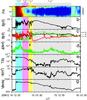 |
Fig. 1 Observations from the ACE and STEREO spacecrafts showing interplanetary structures associated with the event on 2006 December 13. The passage of different structures is indicated by the different colored intervals, i.e., the shock sheath (blue interval “1”), the interplanetary magnetic arcades (pink interval “2”), and the interplanetary CS (yellow interval “3”), as well as the MC (gray interval “4”). Panel a) shows the distribution of electron pitch angles detected by ACE. Panels b) and c) show the magnetic field magnitude and the field components Bx (black line), By (green line), and Bz (red line), in GSM coordinates. The current density calculated from the STEREO A and B magnetic field data is presented in Panel d), in which the current concentrations as denoted by the arrow are believed to originate in the transverse CS during the CME initiation. Panels e) to g) show the corresponding plasma temperature, density, and velocity from ACE observations. |
Figure 1 presents observations from ACE, together with data from STEREO A and B (discussed later in this section). The signed intervals labeled “1–4” and colored by blue, pink, yellow, and gray indicate the passage of the different interplanetary structures of interest, each of which is discussed below.
Panel (a) of Fig. 1 shows the distribution of electron pitch angles at 246 eV, in which the shock and sheath can be easily identified to begin at about 14:00 UT on 2006 December 14 by the isotropic electron pitch angles behaved like the red area in the blue interval “1”. Bidirectional streaming electrons (BDEs) are revealed in the following interplanetary structures (intervals “2–4”). It is well known that the appearance of BDEs along magnetic field lines indicates that both footpoints of the observed magnetic structures connect back to the Sun (e.g., Zwickl et al. 1983; Gosling et al. 1987). Panels (b) and (c) of Fig. 1 show the magnitude of the magnetic field and the three components Bx, By, and Bz, in Geocentric Solar Magnetospheric, or GSM, coordinates. Combined Panels (a), (b) and (c), the CME-related MC (gray interval “4”) are said to have begun at about 22:40 UT on December 14 and connected to the Sun as indicated by BDEs (see also Liu et al. 2008; Rosenvinge et al. 2009). The magnetic structures between the shock sheath and the MC that also connected to the Sun as indicated by the BDEs were interpreted as signatures of nested magnetic loops overlying the MC flux rope by Gosling et al. (1987). Similar to the magnetic arcades overlying the filament system in the Sun, we call the structure after the shock and before the MC as “interplanetary arcades” in this work. From Panel (c), the main magnetic component of the structure between the shock sheath and the MC is directed in the y-direction; i.e., By is the largest component of the field, while the magnetic field of the MC is directed along the z-direction, and Bz dominates in the MC. A CS may often be considered as a boundary between magnetic structures with sheared magnetic fields. In this event, a CS is analyzed to exist ahead of the MC.
It is fortunate that during the time of these observations, the separation of STEREO A and
B is ≈7500 km, which is close enough to permit a calculation of the current density
between the spacecraft based on the magnetic field components from STEREO A/B and an
application of Ampere’s law:  (1)Specifically, we have
 (2)where
BA and
BB are the magnetic fields from STEREO A and B,
and
rA = (xA,yA,zA)
and
rB = (xB,yB,zB)
are the spacecraft locations at the given time.
(2)where
BA and
BB are the magnetic fields from STEREO A and B,
and
rA = (xA,yA,zA)
and
rB = (xB,yB,zB)
are the spacecraft locations at the given time.
The calculated current density profile based on the STEREO A/B satellites is shown in panel (d) of Fig. 1. To compare the observations with the data from the ACE satellite, we shift the STEREO observation 24 min ahead. Panel (d) reveals several peaks in the current. The strongest current density appears in the shock sheath region (interval “1”). At ~21:44 UT, there is a current concentration located just ahead of the MC. According to the calculation results, the structures between the shock sheath and the MC may belong to two parts with one the interplanetary arcades (interval “2”) that correspond to the nested magnetic loops said by Gosling et al. (1987), and the other a CS structure regarded as the interplanetary transverse current sheet (ITCS, interval “3”) in this work. The ITCS is traversed by STEREO A at the location rA = (29.3, −43.0,10.0) RE in GSM coordinates at 21:44 UT on 2006 December 14, and lasts about 10 min (interval “3”). Panels (e)–(g) of Fig. 1 presented the distributions of plasma temperature, density, and velocity detected by ACE. The maximum current density is ≈10-8 A m-2. The speed, hence the thickness of the current sheet, may be calculated based on the average value of the plasma velocity data detected by ACE during this interval. We estimate a thickness ≈5 × 10⁵ km, based on an average velocity ≈841 km s-1 over the interval of ≈10 min. The ITCS thickness is very close to that of a tilted current sheet substructure ahead of a magnetic cloud-like structure, i.e., ~1−4 × 10⁶ km as estimated by Foullon et al. (2007) in the other event. We also notice that there is another current concentration at ~04:30 UT on 2006 December 15 close the center of the MC structure, which may be formed as a result of a clouds kinematic propagation from the Sun to the Earth, without any external forces or influences, as simulated by Owens (2009).
Based on the observations and the results of the previous work (e.g., Zhang et al. 2007a; Liu et al. 2009), the CME on 2006 December 13 is related to a filament system and its overlying multiple magnetic arcades, which may correspond to the relate MC (gray interval “4”) and its ahead interplanetary arcades (pink interval “2”). If so, a natural question is whether the interplanetary current sheet can be found in the CME initiation as pointed by the CME models.
3. Solar surface source of transverse current sheet
 |
Fig. 2 Eruptive event on 2006 December 13 observed on the Solar disk. Panel a) is an MDI image at 01:39 UT showing AR 10930, with a white box indicating the size of the five other panels. Panel b) is a BBSO Hα image at 01:57 UT to show a dark filament (white arrow). The contours on panels b), c), and d) show values of the line-of-sight magnetic field taken from the MDI magnetogram at the closest time with levels of ± (50,100,300,500,1000) G, which also serve to locate the AR neutral line. Panel c) shows an EIT EUV image at 02:12 UT, in which the filament is also visible (white arrow). Panel d) is an EIT EUV image at 03:36, taken after the X3.4 class flare, showing a bright region in post-flare loops (white arrow) where the flare occurred. Panels e) and f) are soft X-ray images from Hinode/XRT, which show an MHD shock wave (white arrow in panel e)) at 02:24 UT, and a plasmoid ejection (white arrow in panel f)) at 02:26 UT, prior to the flare peak. |
The solar source of the CME on 2006 December 13 is observed by multiple wavelengths from the Sun, e.g., the Extreme-Ultraviolet Imaging Telescope (EIT, Delaboudinière et al. 1995) onboard SOHO, the Michelson Doppler Imager (MDI/SOHO, Scherrer et al. 1995), the LASCO/SOHO, and X-Ray Telescope (XRT, Golub et al. 2007) onboard Hinode (Kosugi et al. 2007), as well as Hα/BBSO. Figure 2 presents the on-disk features of the event on 2006 December 13 at four wavelengths. The complex magnetic configurations of the AR/flare is shown in Fig. 2a, an MDI image at 01:39 UT. An AR long filament can be observed along the AR magnetic neutral line in a BBSO Hα image at 01:57 UT (Fig. 2b) and an EIT EUV image at 02:12 UT (Fig. 2c). Post-flare loops appear along the AR neutral line in Fig. 2d of an EIT EUV image at 03:36 UT as indicated by the classic flare model. Above the filament system, there are multiple-layer overlying magnetic arcades whose magnetic fields are perpendicular to that of the filament system. The eruption of the AR filament during the CME launch process can be learned from the bright core of the related CME, which can be observed since 03:06 (Fig. 4c) and may represent erupted filament material (Illing & Hundhausen 1985; Dere et al. 1999). Combined with Fig. 1, the MC in interplanetary space should correspond to the erupted CME-related filament flux rope system (e.g., Wang et al. 2006). The interplanetary arcades (interval “2” in Fig. 1) correspond to the magnetic arcades overlying the filament system on the Sun. Therefore, the ITCS (interval “3” in Fig. 1) should correspond to a CS in the CME solar source, which exists between the related filament system and its overlying magnetic arcades and is tentatively called as a transverse current sheet (TCS). The evidence of the TCS would be found in the XRT observations and the nonlinear force-free extrapolations.
In Figs. 2e and f, there are two interesting Hinode/XRT eruptions in rapid succession during the flare process, which reveal two kinds of blueshifted phenomenon corresponding to an MHD fast-mode shock wave and a plasmoid ejection (Asai et al. 2008 labels the features as “BS2” and “BS1”), and cannot be explained by the simple flare model. The MHD fast-mode shock wave (Fig. 2e) is seen in Hinode/XRT data for the interval 02:22:18–02:26:18, and the plasmoid ejection (Fig. 2f) is seen for the interval 02:24:18-02:28:18. The plasma associated with the MHD shock is heated to more than 2 MK (Asai et al. 2008), which indicates that the physical process generating the MHD shock wave seen as BS2 happened in the higher corona and then the following XRT eruption behaved as BS1. This observational scenario is generally consistent with the picture of double-current sheet reconnection model of Zhang et al. (2006), in which reconnection first takes place at a transverse CS above an active region, and then the reconnection episode occurs at a vertical CS and drives the plasmoid ejection. The existence of a vertical CS is commonly accepted in the current flare/CME initiation model or observations. However, the transverse CS is rarely referred to in the observations though it is often indicated in the CME model (e.g., Antiochos et al. 1999; Zhang et al. 2005; Zhang 2006; Zhang & Wang 2007b). Based on the nonlinear force-free field (NLFFF) models, we constructed the coronal magnetic field in AR 10930 and continue to scrutinize and diagnose the CSs.
A recent workshop (Schrijver et al. 2008) used
photospheric vector magnetic field values obtained with the Solar Optical Telescope (SOT) on
Hinode to construct the coronal magnetic field in AR 10930 based on different NLFFF models.
Here we examine the magnetic field models constructed using the current-field iteration
method of Wheatland (2007), which was judged to
provide the most successful reconstructions at the workshop based on a variety of
criteria (see Schrijver et al. 2008). Two models are
available, providing magnetic field models at 20:30 UT on 2006 December 12 (before the
X3.4 flare) and at 04:30 UT on December 13 (after the flare). The model constructed before
the flare is referred to in Schrijver et al. (2008)
as the  model. Using
these two models, we calculated the current density profile around the AR before and after
the flare to investigate the existing current structures.
model. Using
these two models, we calculated the current density profile around the AR before and after
the flare to investigate the existing current structures.
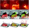 |
Fig. 3 Comparisons between the extrapolation structures and the XRT observations. The first row: the XRT observation at 20:30 on 2006 December 12 before the X3.4 flare (panels a), b)) and at 04:30 UT on 2006 December 13 after the flare (panel c)). The white rectangle in panel a) shows the field of view of the seven other panels. Second row: visualizations of the sample closed field lines (red) and the iso-surface of the current density at the level of 6.96 mA m-2 (green) within the NLFFF model volume (Wheatland 2007) at 20:30 UT on December 12 and at 04:30 UT on December 13, shown against the corresponding map of Hinode/SP Bz at the photosphere (panel d)) and at a height of z = 1371 km (panels e) and f)). The last row shows the 3D images of the middle row. The transverse CS (yellow arrows) and the vertical one (white arrows) can be clearly identified in panel h). |
Figure 3 presents the XRT observations (top row) in comparison with the extrapolations (bottom two rows) before [left two columns] and after the flare (right column). The white rectangle in panel (a) denotes the field of view of the other eight panels. The second row shows the sample’s closed field lines within the NLFFF model volume, together with the iso-surfaces of the inferred current density at the magnitude of 6.96 mA m-2, against the corresponding maps of Hinode/SP Bz at the photosphere (panel (d)) and at the height of z = 1371 km (panels (e) and (f)). The sample’s closed field lines are similar to the simultaneous XRT loops in morphology. The 3D view of the middle row is shown at the bottom row, in which a transverse CS and a vertical one are revealed above the AR neutral line before the X3.4 flare. It is interesting that the transverse CS from the NLFFF model just corresponds to the XRT brightness increase in panel (b), and they are located in the same coronal height range that can reach ~35 Mm. After the flare, the top sample field lines and the transverse CS leave the NLFFF mode volume, and the bottom field lines ascend to new heights, as well as the vertical CS became short in the projection at the photosphere (cf. panels (h) and (i)). The AR magnetic configurations was reconstructed and showed more potential, suggesting the release of magnetic energy associated with reconnection.
The vertical and transverse CSs are indicated in the XRT eruptions and are reconstructed based on NLFFF mode. Just like the vertical CS in the post-CME, CS behaved like the bright ray-like features (e.g., Lin et al. 2007, 2009), so we wonder whether the TCS can show white-light evidence in SOHO/LASCO observations. Figure 4 are the base-difference images of the LASCO CME, in each of which a pre-event image at 02:06 UT is subtracted. The CME first appeared at 02:30 UT (Fig. 4a), and had been a nearly complete halo since 02:54 UT (see also Liu et al. 2008). According to the LASCO CME catalog1, the X3.4 flare-associated CME has a projection speed of ≈1774 km s-1 and a deceleration of ≈61 m s-2. From 02:54 to 04:42 UT, a brightness increase at the CME front remains compact and undispersed during its propagation from ≈4 R⊙ to >10 R⊙. Figure 4i combines the LASCO observations at different moments to show the sequence propagations of the brightness increase.
The X3.4 flare-associated CME first appeared very weak in the LASCO field of view at 02:30 UT and can be identified in a very restricted range of [–5, 5] (see Fig. 4a). The CME presented clear white-light coronal loop structures, which may correspond to the overlying magnetic arcades above the filament system. Since 02:54 UT, a brightness increase have been observed at the CME bright front. At 03:06 UT, the CME’s bright core (Fig. 4c) first appeared and represent the erupted filament system. Therefore, the brightness increase propagating at the CME front is located above the filament and under the top magnetic arcades overlying the filament, i.e., have a consistent position with the TCS deduced by the related ITCS. As shown in the middle panel of Fig. 1 in Liu et al. (2008), the CS-like brightness increase is situated behind the surrounding CME faint front, which is said to be density enhancements induced by the fast-mode MHD shock (e.g., Vourlidas et al. 2003; Liu et al. 2008). Lugaz et al. (2005) simulated a streamer-associated CME eruption, in which two features, i.e., a concave-outward indentation and a brightness increase in the line-of-sight images that are caused by the front shock and the related behind reverse shocks, can be observed, but appear only in front-side CMEs. While for the CME on 2006 December 13, it is earth-directed, and the concave-outward indentation did not appear in LASCO/C3 images. Therefore, we find that the brightness increase in the LASCO observations might correspond to a TCS during the CME initiation.
 |
Fig. 4 CME base-difference images from SOHO/LASCO at different moments. A pre-event image at 02:06 UT has been subtracted in each case. The solid arrows denote a brightness increase at the CME front. The CME bright core (dashed arrow) appeared at 03:06 UT in panel c). Panels a)–h) have the same size of windows. Panel i) combined the CME difference images from 02:54 to 04:42 UT, during which a bright increase at the CME front can be traced (see the solid lines). The white circle denotes the Sun. |
Table 1 summarizes the timing of the various observations presented here, which proves that the TCS exists. The table distinguishes between the direct observations and the interpretations we gave them.
Timing of observations and their interpretation.
 |
Fig. 5 CME eruption and propagation from the solar source to interplanetary space. Panels a) and b): two cartoons with extrapolation field lines by the method of Wang (2001), shown against MDI magnetograms, illustrating the the field evolutions before and after the flare. The field configurations of AR 10930 include the top magnetic arcades (red), the transverse CS (top green), the filament system (light and thick blue), and the AR neutral line (yellow dashed), as well as the vertical CS (green rectangle in panel b)) to be elongated. Panel c): a cartoon illustrates the CME related interplanetary structures, which are shock (black dashed), shock sheath, the interplanetary arcades (red), and the interplanetary transverse CS (ITCS, green), and the MC (blue). The long black arrow denotes the direction along which STEREO or ACE traversed the shock and the MC. |
The CME eruption and propagation from the solar source to interplanetary space can be explained in the cartoon of Fig. 5. The field lines in panel (a) are from the NLFFF extrapolation by the model of Wang et al. (2001) based on the MDI magnetogram at 01:39 on December 13, which can provide a larger field of view than in the method of Wheatland (2007). As shown in panel (a), the CME related initial reconnection occurs at the transverse CS, which is located between the top arcade system and the bottom flux rope system with its embedded filament. Accompanying the first reconnection, the existing AR loop system is reconfigured, producing the fast-mode MHD shock observed in the XRT data (e.g. Asai et al. 2008), and the filament system loses its equilibrium. The filament lifts off due to the action of magnetic buoyancy. The field lines and the vertical CS panel (b) below the filament flux system become elongated. At the vertical CS, the other reconnection or topology collapses, producing profound changes in the geometry and topology of the AR flux systems and explosive energy release, namely the X3.4 class flare. The post-flare loops quickly appear and expand above the AR neutral line, manifesting the continuous localized energy release in this interval. Panel (c) of Fig. 5 illustrates the passage of the CME through interplanetary space, which shows the various interplanetary structures, namely the shock, the following shock sheath, the interplanetary arcades, and the interplanetary transverse CS (ITCS) between the interplanetary arcades and the MC. STEREO or ACE traversed the shock and the MC in the direction indicated. The interplanetary arcades and the MC, of which the magnetic fields present almost perpendicular in the ACE observations, have good correspondence to the top magnetic arcades and the bottom flux rope system with the embedded filament in the CME solar source.
4. Conclusion and discussion
Tracing current sheets from the solar atmosphere to interplanetary space during a solar eruptive event is a difficult task. Even a CS identified in interplanetary space, it could not exclude its formation due to the interaction between the ICME, the other trailing ICME, and the ambient solar wind plasma, etc. (Foullon et al. 2007; Owens 2009). This paper presents evidence of the current sheets for the extreme flare/CME event of 2006 December 13. We prove that a transverse CS can be identified and traced from the Sun to the inner heliosphere for this event in the following direct and/or indirect ways.
First, the in-situ STEREO observations confirm a current concentration at 21:44 UT, which is situated at the boundary between the interplanetary magnetic arcades and the magnetic cloud. It is argued that this interplanetary CS corresponds to the transverse CS identified in the CME source, and said that the interplanetary magnetic arcades are the interplanetary counterpart of the overall loops above the active region, while the magnetic cloud is the expanded flux rope associated to the filament in the active region.
Second, in the pre-flare state, observations by Hinode/XRT showing a shock and ejecta
indicate magnetic reconnections at the site of two current sheets – a transverse CS lying
above the AR and a vertical current sheet above the AR magnetic neutral line, respectively.
In support of these identifications, transverse and vertical current structures are found in
3D nonlinear force-free vector, magnetic field models constructed from Hinode/SOT vector
magnetograms (in particular, using the model described by
Schrijver et al. (2008). It is noted that the recent
nonlinear force-free extrapolations constructed by other researchers also show the same
features to support the reality of the inferred current sheets (e.g., Kataoka et al. 2009).
Third, the brightness increase in the CME front may be evidence of CS in LASCO observations.
Fourth, the timing of the various identifications and indications of the TCS and of its propagation provide a consistent picture of overall physical processes occurring in this Sun-Earth connection event. In the LASCO images, the CS-like brightness increase is observed without dispersion to accompany the CME appearance from 02:54 to 04:42 UT, after which the CME front propagates almost out of the LASCO field of view. The reason the TCS survives may be that the basic topology in the large-scale magnetic fields do not change, though reconnection may take place in small and narrow diffusion regions. The flare/CME current sheet is too thick as far as we know, e.g., 104−105 km from (Lin et al. 2009), which could not be totally destroyed in a short time in fact. According to Lin et al. (2009), we can estimate the time intervals for CME-related CSs’ diffusing away in the other two events on 2003 November 18 and on 2002 January 8, in which the electric resistivity ηe and the thickness of the related current sheet d are provided. The diffusing time can be approximately calculated as τ = d2/η, where the magnetic diffusivity η = ηe/μ0. The results show that the CME-related CSs would be diffused away after 3 days. This may be why the solar CS can be observed in interplanetary space.
The identification and evolution of the two current sheets in this paper may provide new observational information for understanding CME mechanisms. However, more careful CS diagnosis based on well-designed multi-domain observations is required to confirm the results and interpretations presented here, and it is desirable to repeat the investigation with more CME events. In addition, it is important to make closer comparison with CME models regarding the reconnection processes. Additional observational studies and further comparison with models may lead to progress in understanding solar eruptive events.
Acknowledgments
We are grateful to all members of the SOHO EIT, LASCO, and MDI teams, to the STEREO, ACE, Wind, and Hinode teams, as well as to the BBSO staff for providing the wonderful data. The authors are also thankful to J. Luhmann at UCB/SSL and CDAWeb. SOHO is a project of international cooperation between ESA and NASA. Hinode is a Japanese mission developed and launched by ISAS/JAXA, with NAOJ as a domestic partner and NASA and STFC (UK) as international partners. The work is supported by National Natural Science Foundation of China (10603008, 10973019, 40636031, 40974104, 40731056, 40974112, 10873020, 40674081, 40890161, 10703007, 10733020, 11003024, and 11003026), Doctoral Fund of Ministry of Education of China (20090001110012), National Science Fund for Distinguished Young Scholars (11025315), and National Key Basic Research Science Foundation (2011CB811400).
References
- Antiochos, S. K., Devore, C. R., & Klimchuk, J. A. 1999, ApJ, 510, 485 [Google Scholar]
- Asai, A., Hara, H., Watanabe, T., et al. 2008, ApJ, 685, 622 [NASA ADS] [CrossRef] [Google Scholar]
- Bemporad, A., Poletto, G., Suess, S. T., et al. 2006, ApJ, 638, 1110 [Google Scholar]
- Burlaga, L., Sittler, E., Mariani, F., & Schwenn, R. 1981, J. Geophys. Res., 86(A8), 6673 [Google Scholar]
- Brueckner, G. E., Howard, R. A., Koomen, M. J., et al. 1995, Sol. Phys., 162, 357 [NASA ADS] [CrossRef] [Google Scholar]
- Carmichael, H. 1964, in The Physics of Solar Flares, ed. W. N. Hess (Washington, DC: NASA), 451 [Google Scholar]
- Ciaravella, A., Raymond, J. C., Li, J., et al. 2002, ApJ, 575, 1116 [NASA ADS] [CrossRef] [Google Scholar]
- Chen, P. F., & Shibata, K. 2000, ApJ, 545, 524 [Google Scholar]
- Dere, K. P., Brueckner, G. E., Howard, R. A., Michels, D. J., & Delaboudiniére, J.-P. 1999, ApJ, 516, 465 [NASA ADS] [CrossRef] [Google Scholar]
- Delaboudinière, J.-P., Artzner, G. E., Brunaud, J., et al. 1995, Sol. Phys., 162, 291 [NASA ADS] [CrossRef] [Google Scholar]
- Domingo, V., Fleck, B., & Poland, A. I. 1995, Sol. Phys., 162, 1 [NASA ADS] [CrossRef] [Google Scholar]
- Foullon, C., Owen, C. J., Dasso, S., et al. 2007, Sol. Phys., 244, 139 [NASA ADS] [CrossRef] [Google Scholar]
- Forbes, T. G. 2000, J. Geophys. Res., 105, A10, 23153 [Google Scholar]
- Golub, L., Deluca, E., Austin, G., et al. 2007, Sol. Phys.., 243, 63 [NASA ADS] [CrossRef] [Google Scholar]
- Gosling, J. T. 1997, Coronal mass ejections: an overview, in Coronal Mass Ejections, ed. N. Crooker, J. A. Joselyn, & J. Feynman, AGU Geophys. Monog., 99, 9 [Google Scholar]
- Gosling, J. T., Baker, D. N., Bame, S. J., et al. 1987, J. Geophys. Res., 92, 8519 [Google Scholar]
- Guo, Y., & Ding, M. D. 2008, ApJ, 679, 1629 [NASA ADS] [CrossRef] [Google Scholar]
- Harris, E. G. 1962, Nuovo Cimento, 23, 115 [Google Scholar]
- Heyvaerts, J., Priest, E. R., & Rust, D. M. 1977, ApJ, 216, 123 [NASA ADS] [CrossRef] [Google Scholar]
- Hirayama, T. 1974, Sol. Phys., 34, 323 [NASA ADS] [CrossRef] [Google Scholar]
- Illing, R. M. E., & Hundhausen, A. J. 1985, J. Geophys. Res., 90, 275 [Google Scholar]
- Imada, S., Hara, H., Watanabe, T., et al. 2008, ApJ, 679, L155 [NASA ADS] [CrossRef] [Google Scholar]
- Jing, J., Wiegelmann, T., Suematsu, Y., Kubo, M., & Wang, H. M. 2008a, ApJ, 676, L81 [NASA ADS] [CrossRef] [Google Scholar]
- Jing, J., Chae, J., & Wang, H. M. 2008b, ApJ, 672, L73 [NASA ADS] [CrossRef] [Google Scholar]
- Kataoka, R., Ebisuzaki, T., Kusano, K., et al. 2003, J. Geophys. Res., 114, 10102 [CrossRef] [Google Scholar]
- Ko, Y.-K., Raymond, J. C., Lin, J., et al. 2003, ApJ, 594, 1068 [NASA ADS] [CrossRef] [Google Scholar]
- Kohl, J. L., Esser, R., Gardner, L. D., et al. 1995, Sol. Phys., 162, 313 [NASA ADS] [CrossRef] [Google Scholar]
- Kopp, R. A., & Pneuman, G. W. 1976, Sol. Phys., 50, 85 [NASA ADS] [CrossRef] [Google Scholar]
- Kosugi, T., Matsuzaki, K., Sakao, T., et al. 2007, Sol. Phys., 243, 3 [NASA ADS] [CrossRef] [Google Scholar]
- Kubo, M., Yokoyama, T., Katsukawa, Y., et al. 2007, PASJ, 59, S779 [NASA ADS] [Google Scholar]
- Lin, J., & Forbes, T. G. 2000, J. Geophys. Res., 105, 2375 [NASA ADS] [CrossRef] [Google Scholar]
- Lin, J., Li, J., Forbes, T. G., et al. 2007, ApJ, 658, L123 [Google Scholar]
- Lin, J., Li, J., Ko, Y.-K., & Raymond, J. C. 2009, ApJ, 693, 1666 [NASA ADS] [CrossRef] [Google Scholar]
- Liu, Y., Luhmann, J. G., Müller-Mellin, R., et al. 2008, ApJ, 689, 563 [NASA ADS] [CrossRef] [Google Scholar]
- Lugaz, N., Manchester IV, W. B., & Gombosi, T. I. 2005, ApJ, 627, 1019 [Google Scholar]
- Mikić, Z., & Linker, J. 1994, ApJ, 430, 898 [Google Scholar]
- Moore, R. L., LaRosa, T. N., & Orwig, L. E. 1995, ApJ, 438, 985 [NASA ADS] [CrossRef] [Google Scholar]
- Moore, R. L., Sterling, A. C., Hudson, H. S., & Lemen, J. R. 2001, ApJ, 552, 833 [NASA ADS] [CrossRef] [Google Scholar]
- Ning, Z. J. 2008, Sol. Phys., 247, 53 [NASA ADS] [CrossRef] [Google Scholar]
- Owens, M. J. 2009, Sol. Phys., 260, 207 [NASA ADS] [CrossRef] [Google Scholar]
- Raymond, J. C., Ciaravella, A., Dobrzycka, D., et al. 2003, ApJ, 597, 1106 [NASA ADS] [CrossRef] [Google Scholar]
- Scherrer, P. H., Bogart, R. S., Bush, R. I., et al. 1995, Sol. Phys., 162, 129 [Google Scholar]
- Schrijver, C. J., DeRosa, M. L., Metcalf, T., et al. 2008, ApJ, 675, 1637 [Google Scholar]
- Shibata, K. 1999, Ap&SS, 264, 129 [NASA ADS] [CrossRef] [Google Scholar]
- Shibata, K., Masuda, S., Shimojo, M., et al. 1995, ApJ, 451, L83 [NASA ADS] [CrossRef] [Google Scholar]
- Sturrock, P. A. 1966, Nature, 221, 695 [NASA ADS] [CrossRef] [Google Scholar]
- Sturrock, P. A., Kaufman, P., Moore, R. L., & Smith, D. F. 1984, Sol. Phys., 94, 341 [NASA ADS] [CrossRef] [Google Scholar]
- Tsuneta, S. 1997, ApJ, 483, 507 [NASA ADS] [CrossRef] [Google Scholar]
- von Rosenvinge, T. T., Richardson, I. G., Reames, D. V., et al. 2009, Sol. Phys., 256, 443 [NASA ADS] [CrossRef] [Google Scholar]
- Vourlidas, A., Wu, S. T., Wang, A. H., Subramanian, P., & Howard, R. A. 2003, ApJ, 598, 1392 [NASA ADS] [CrossRef] [Google Scholar]
- Wang, H., Yan, H., & Sakurai, T. 2001, Sol. Phys., 201, 323 [NASA ADS] [CrossRef] [Google Scholar]
- Wang, Y. M., Zhou, G. P., Ye, P. Z., Wang, S., & Wang, J. X. 2006, ApJ, 651, 1245 [NASA ADS] [CrossRef] [Google Scholar]
- Webb, D. F., Burkepile, J., Forbes, T. G., & Riley, P. 2003, J. Geophys. Res., 108 (A12), 1440 [Google Scholar]
- Wheatland, M. S. 2007, Sol. Phys., 245, 251 [NASA ADS] [CrossRef] [Google Scholar]
- Yan, Y., Huang, J., & Chen, B. 2007, PASJ, 59, S815 [NASA ADS] [Google Scholar]
- Zhang, J., Li, L. P., & Song, Q. 2007a, ApJ, 662, L35 [NASA ADS] [CrossRef] [Google Scholar]
- Zhang, Y.-Z., Hu, Y.-Q., & Wang, J.-X. 2005, ApJ, 626, 1096 [NASA ADS] [CrossRef] [Google Scholar]
- Zhang, Y.-Z., Wang, J.-X., & Hu, Y.-Q. 2006, ApJ, 641, 572 [NASA ADS] [CrossRef] [Google Scholar]
- Zhang, Y.-Z., & Wang, J.-X. 2007b, ApJ, 663, 592 [NASA ADS] [CrossRef] [Google Scholar]
- Zwickl, R. D., Asbridge, J. R., Bame, S. J., et al. 1983, in Solar Wind Five; NASA ed. M. Eugebauer, (Washington, DC: NASA), Conf. Proc. 2280, 711 [Google Scholar]
All Tables
All Figures
|
Fig. 1 Observations from the ACE and STEREO spacecrafts showing interplanetary structures associated with the event on 2006 December 13. The passage of different structures is indicated by the different colored intervals, i.e., the shock sheath (blue interval “1”), the interplanetary magnetic arcades (pink interval “2”), and the interplanetary CS (yellow interval “3”), as well as the MC (gray interval “4”). Panel a) shows the distribution of electron pitch angles detected by ACE. Panels b) and c) show the magnetic field magnitude and the field components Bx (black line), By (green line), and Bz (red line), in GSM coordinates. The current density calculated from the STEREO A and B magnetic field data is presented in Panel d), in which the current concentrations as denoted by the arrow are believed to originate in the transverse CS during the CME initiation. Panels e) to g) show the corresponding plasma temperature, density, and velocity from ACE observations. |
| In the text | |
|
Fig. 2 Eruptive event on 2006 December 13 observed on the Solar disk. Panel a) is an MDI image at 01:39 UT showing AR 10930, with a white box indicating the size of the five other panels. Panel b) is a BBSO Hα image at 01:57 UT to show a dark filament (white arrow). The contours on panels b), c), and d) show values of the line-of-sight magnetic field taken from the MDI magnetogram at the closest time with levels of ± (50,100,300,500,1000) G, which also serve to locate the AR neutral line. Panel c) shows an EIT EUV image at 02:12 UT, in which the filament is also visible (white arrow). Panel d) is an EIT EUV image at 03:36, taken after the X3.4 class flare, showing a bright region in post-flare loops (white arrow) where the flare occurred. Panels e) and f) are soft X-ray images from Hinode/XRT, which show an MHD shock wave (white arrow in panel e)) at 02:24 UT, and a plasmoid ejection (white arrow in panel f)) at 02:26 UT, prior to the flare peak. |
| In the text | |
|
Fig. 3 Comparisons between the extrapolation structures and the XRT observations. The first row: the XRT observation at 20:30 on 2006 December 12 before the X3.4 flare (panels a), b)) and at 04:30 UT on 2006 December 13 after the flare (panel c)). The white rectangle in panel a) shows the field of view of the seven other panels. Second row: visualizations of the sample closed field lines (red) and the iso-surface of the current density at the level of 6.96 mA m-2 (green) within the NLFFF model volume (Wheatland 2007) at 20:30 UT on December 12 and at 04:30 UT on December 13, shown against the corresponding map of Hinode/SP Bz at the photosphere (panel d)) and at a height of z = 1371 km (panels e) and f)). The last row shows the 3D images of the middle row. The transverse CS (yellow arrows) and the vertical one (white arrows) can be clearly identified in panel h). |
| In the text | |
|
Fig. 4 CME base-difference images from SOHO/LASCO at different moments. A pre-event image at 02:06 UT has been subtracted in each case. The solid arrows denote a brightness increase at the CME front. The CME bright core (dashed arrow) appeared at 03:06 UT in panel c). Panels a)–h) have the same size of windows. Panel i) combined the CME difference images from 02:54 to 04:42 UT, during which a bright increase at the CME front can be traced (see the solid lines). The white circle denotes the Sun. |
| In the text | |
|
Fig. 5 CME eruption and propagation from the solar source to interplanetary space. Panels a) and b): two cartoons with extrapolation field lines by the method of Wang (2001), shown against MDI magnetograms, illustrating the the field evolutions before and after the flare. The field configurations of AR 10930 include the top magnetic arcades (red), the transverse CS (top green), the filament system (light and thick blue), and the AR neutral line (yellow dashed), as well as the vertical CS (green rectangle in panel b)) to be elongated. Panel c): a cartoon illustrates the CME related interplanetary structures, which are shock (black dashed), shock sheath, the interplanetary arcades (red), and the interplanetary transverse CS (ITCS, green), and the MC (blue). The long black arrow denotes the direction along which STEREO or ACE traversed the shock and the MC. |
| In the text | |
Current usage metrics show cumulative count of Article Views (full-text article views including HTML views, PDF and ePub downloads, according to the available data) and Abstracts Views on Vision4Press platform.
Data correspond to usage on the plateform after 2015. The current usage metrics is available 48-96 hours after online publication and is updated daily on week days.
Initial download of the metrics may take a while.