© ESO, 2010

1. Introduction

A fundamental test of cosmological models is provided by the distribution of nonlinear virialized objects, such as galaxies or clusters of galaxies. First, this allows to check that nonlinear objects form through the amplification by gravitational instability of small (nearly Gaussian) primordial density fluctuations (Peebles 1980). Second, quantitative comparisons between theoretical predictions and observations allow to derive constraints on cosmological parameters (Zheng & Weinberg 2007). Indeed, observations show that galaxies and clusters do not follow a Poisson distribution but show significant large-scale correlations (e.g., McCracken et al. 2008; Padilla et al. 2004). In particular, at large scales their two-point correlation function is roughly proportional to the underlying matter correlation, with a multiplicative factor b², called the bias, that is greater for more massive objects.

Following the spirit of the Press-Schechter picture (Press & Schechter 1974), where nonlinear virialized objects are identified with high-density fluctuations in the initial (linear) density field, Kaiser (1984) showed how such a behavior for the halo correlation naturally arises. Similar results are obtained for the clustering of density peaks instead of overdensities above a given threshold (Bardeen et al. 1986). Indeed, distant high-density regions are correlated through their common longwavelength modes of the linear density field, and the effect is greater for more massive and extreme objects. A somewhat simpler derivation can be obtained through the peak-background split argument (Cole & Kaiser 1989; Bond et al. 1991). This rests on the same physics, which is that within a large region characterized by a positive mean density contrast local density peaks beyond a given density threshold are more frequent than in the mean, which yields a positive correlation between rare massive halos and the larger-scale matter density field.

Along these lines, a simple analytical model that compares reasonably well with numerical simulations was presented by Mo & White (1996), while a better agreement was obtained by Sheth & Tormen (1999), at the cost of adding a few parameters fitted to the simulations (through the halo mass function). More complex models, that also apply to redshift space and take into account subleading scale-dependent terms can be found for instance in Desjacques (2008); Desjacques & Sheth (2010). On the other hand, various fitting formulas have been proposed from measures in numerical simulations (Hamana et al. 2001; Pillepich et al. 2010; Tinker et al. 2010; Manera et al. 2010). In particular, Tinker et al. (2010) have recently studied the dependence of the halo bias on the density contrast δ_∗ used to define the halos. In the paper we present a simple analytical model for the halo bias that extends a previous work (Valageas 2009) to arbitrary density thresholds in the range 200 ≤ δ_∗ ≤ 1600. This is of practical interest as the definition of halos can vary among authors, and it can happen that observations only extend to smaller radii than the usual virial radius, which corresponds to objects defined by higher density thresholds. In addition, we also improve on Valageas (2009) by simplifying somewhat the model, especially the treatment of halo motions, while obtaining a better accuracy for low-mass halos. This should allow an easier generalization to more complex cases, such as non-Gaussian initial conditions. This simple model also allows us to evaluate the inaccuracies implied by two approximations that are frequently used, that is, neglecting halo motions and linearizing the halo correlation function over the matter correlation function.

In Sect. 2 we describe our model for the bias of halos defined by a nonlinear density contrast δ_∗ = 200. We explain how the standard model of Kaiser (1984) for the correlation of rare massive halos is modified once we take into account the motion of halos. Then, we point out that normalization conditions can be very useful to constrain the bias of intermediate and low mass halos, which allows to build a simple and efficient model. Next, we show that we obtain a good agreement with numerical simulations. In Sect. 3 we extend this model for the bias, as well as for the halo mass function, to the case of halos defined by a larger nonlinear density contrast, and we compare our results with numerical simulations for 200 ≤ δ_∗ ≤ 1600. Finally, we estimate the importance of halo motions and of the nonlinearity of the bias in Sects. 4 and 5, and we conclude in Sect. 6.

2. Bias of dark matter halos

Following Kaiser (1984) we estimate the two-point correlation function of dark matter halos, whence their bias, from the probability to reach a linear density threshold δ_L ∗  (associated with the formation of virialized halos of nonlinear density contrast δ_∗). As in Valageas (2009), we improve this model by taking into account the motion of halos, associated with the change from Lagrangian to Eulerian space (i.e., from the linear density field to the actual nonlinear density field). However, we simplify the prescription used in Valageas (2009) as we no longer use a spherical collapse model to estimate these displacements but use the initial momenta of both halos (i.e., the linear displacement field). In addition, we add a further ingredient to the study of Valageas (2009), as we explicitly enforce the normalization to unity of the halo bias (when integrated over all halo masses). We describe below this simple model.

2.1. Lagrangian space

We first consider the two-point correlation function of halos in Lagrangian space, that is within the linear density field δ_L(q), where we identify future halos of Eulerian radius r and nonlinear density contrast δ_∗ (with typically δ_∗ ~ 200) with spherical regions of Lagrangian radius q and linear density contrast δ_L ∗ . Thanks to the conservation of mass, the Lagrangian and Eulerian properties of halos of mass M are related by $\mathit{M}\mathrm{=}\frac{\mathrm{4}\mathit{\pi }}{\mathrm{3}}\overline{\mathit{\rho }}\hspace{0.17em}{\mathit{q}}^{\mathrm{3}}\mathit{,}{\mathit{q}}^{\mathrm{3}}\mathrm{=}\mathrm{(}\mathrm{1}\mathrm{+}{\mathit{\delta }}_{\mathrm{\ast }}\mathrm{)}\hspace{0.17em}{\mathit{r}}^{\mathrm{3}}\mathrm{and}{\mathit{\delta }}_{\mathrm{\ast }}\mathrm{=}\mathrm{ℱ}\mathrm{\left(}{\mathit{\delta }}_{\mathrm{L}\mathrm{\ast }}\mathrm{\right)}\mathit{,}$(1)where $\overline{\mathit{\rho }}$ is the mean matter density. As pointed out in Valageas (2009), the function ℱ describes the spherical collapse dynamics, so that in a ΛCDM cosmology with Ω_m = 0.27, Ω_Λ = 0.73, we have δ_L ∗  ≃ 1.59 at z = 0 for δ_∗ = 200, instead of the usual value δ_c ≃ 1.675 associated with full collapse to a point, that is with δ_∗ = ∞.

Defining halos by the linear threshold δ_L ∗  = ℱ^-1(δ_∗), rather than by the full collapse value δ_c, is closer to observational and numerical procedures, since (in the best cases) one defines “halos” in galaxy or cluster surveys, and in numerical simulations, by the radius and mass of overdensities within a given nonlinear density threshold δ_∗. Moreover, this gives the freedom to chose different thresholds, such as δ_∗ = 200 or 100 (Valageas 2009). As discussed in Sect. 3 in Valageas (2009), for massive (M ~ 10¹⁵   h^-1M_⊙) and rare halos, the choice δ_∗ = 200 also roughly corresponds to the separation between outer shells, dominated by radial accretion, and inner shells, with a significant transverse velocity dispersion, that have experienced shell crossing. The case of typical halos (i.e. below the knee of the halo mass function) is more intricate as they do not show such a clear separation. This can also be seen in numerical simulations, such as Fig. 3 in Cuesta et al. (2008). At high redshift, where nonlinear objects have a smaller mass, this “virialization” radius shifts to higher density contrasts for ΛCDM cosmologies, because of the change of slope of the linear matter power spectrum with scale (e.g., δ_∗ ~ 500 for M ~ 10¹¹   h^-1M_⊙, as seen in Fig. 5 in Valageas 2009).

Then, defining the halo correlation as the fractional excess of halo pairs (Kaiser 1984; Peebles 1980), we write in Lagrangian space $\begin{array}{ccc}{\overline{\mathit{n}}}_{\mathrm{L}}\mathrm{\left(}{\mathit{M}}_{\mathrm{1}}\mathit{,}{\mathit{M}}_{\mathrm{2}}\mathrm{;}{s}\mathrm{1}\mathit{,}{s}\mathrm{2}\mathrm{\right)}\mathrm{d}{\mathit{M}}_{\mathrm{1}}\mathrm{d}{\mathit{M}}_{\mathrm{2}}\mathrm{d}{s}\mathrm{1}\mathrm{d}{s}\mathrm{2}& \mathrm{=}& \\ & & {\overline{\mathit{n}}}_{\mathrm{L}}\mathrm{\left(}{\mathit{M}}_{\mathrm{1}}\mathrm{\right)}{\overline{\mathit{n}}}_{\mathrm{L}}\mathrm{\left(}{\mathit{M}}_{\mathrm{2}}\mathrm{\right)}\mathrm{[}\mathrm{1}\mathrm{+}{\mathit{\xi }}_{\mathrm{L}}\mathrm{(}{\mathit{M}}_{\mathrm{1}}\mathit{,}{\mathit{M}}_{\mathrm{2}}\mathrm{;}\mathit{s}\mathrm{\left)}\mathrm{\right]}\mathrm{d}{\mathit{M}}_{\mathrm{1}}\mathrm{d}{\mathit{M}}_{\mathrm{2}}\mathrm{d}{s}\mathrm{1}\mathrm{d}{s}\mathrm{2}\mathit{.}\end{array}$(2)Here and in the following we use the letter s for the position of halos in Lagrangian space to avoid confusion with their Lagrangian radius q, and we introduced the Lagrangian distance, s =  |s₂ − s₁| , between both objects. We also note with a subscript L the quantities associated with the linear fields or the Lagrangian space. Then, following Kaiser (1984) and Valageas (2009), we obtain the fractional excess of halo pairs from the bivariate density distribution over the two spheres of radii q₁ and q₂, $\begin{array}{ccc}\mathrm{1}\mathrm{+}{\mathit{\xi }}_{\mathrm{L}}\mathrm{\left(}{\mathit{M}}_{\mathrm{1}}\mathit{,}{\mathit{M}}_{\mathrm{2}}\mathrm{;}\mathit{s}\mathrm{\right)}& \mathrm{=}& \frac{{\mathrm{𝒫}}_{\mathrm{L}}\mathrm{\left(}{\mathit{\delta }}_{\mathrm{L}\mathrm{1}}\mathit{,}{\mathit{\delta }}_{\mathrm{L}\mathrm{2}}\mathrm{\right)}}{{\mathrm{𝒫}}_{\mathrm{L}}\mathrm{\left(}{\mathit{\delta }}_{\mathrm{L}\mathrm{1}}\mathrm{\right)}{\mathrm{𝒫}}_{\mathrm{L}}\mathrm{\left(}{\mathit{\delta }}_{\mathrm{L}\mathrm{2}}\mathrm{\right)}}\\ & & \mathrm{=}\frac{{\mathit{\sigma }}_{\mathrm{1}}{\mathit{\sigma }}_{\mathrm{2}}}{\sqrt{{\mathit{\sigma }}_{\mathrm{1}}^{\mathrm{2}}{\mathit{\sigma }}_{\mathrm{2}}^{\mathrm{2}}\mathrm{-}{\mathit{\sigma }}_{\mathrm{12}}^{\mathrm{4}}}}\hspace{0.17em}\exp \left(\frac{{\mathit{\delta }}_{\mathrm{L}\mathrm{\ast }}^{\mathrm{2}}{\mathit{\sigma }}_{\mathrm{12}}^{\mathrm{2}}\mathrm{(}\mathrm{2}\mathrm{-}{\mathit{\sigma }}_{\mathrm{12}}^{\mathrm{2}}\mathit{/}{\mathit{\sigma }}_{\mathrm{1}}^{\mathrm{2}}\mathrm{-}{\mathit{\sigma }}_{\mathrm{12}}^{\mathrm{2}}\mathit{/}{\mathit{\sigma }}_{\mathrm{2}}^{\mathrm{2}}\mathrm{)}}{\mathrm{2}\mathrm{(}{\mathit{\sigma }}_{\mathrm{1}}^{\mathrm{2}}{\mathit{\sigma }}_{\mathrm{2}}^{\mathrm{2}}\mathrm{-}{\mathit{\sigma }}_{\mathrm{12}}^{\mathrm{4}}\mathrm{)}}\right)\mathit{,}\end{array}$where we considered a single population, that is halos defined by the same density thresholds δ_L ∗  and δ_∗ = ℱ(δ_L ∗ ). Here we assumed Gaussian initial conditions and we introduced the cross-correlation of the smoothed linear density contrast at scales q₁ and q₂, at positions s₁ and s₂, $\begin{array}{ccc}{\mathit{\sigma }}_{{\mathit{q}}_{\mathrm{1}}\mathit{,}{\mathit{q}}_{\mathrm{2}}}^{\mathrm{2}}\mathrm{\left(}\mathit{s}\mathrm{\right)}& \mathrm{=}& \mathrm{⟨}{\mathit{\delta }}_{\mathrm{L}{\mathit{q}}_{\mathrm{1}}}\mathrm{\left(}{s}\mathrm{1}\mathrm{\right)}{\mathit{\delta }}_{\mathrm{L}{\mathit{q}}_{\mathrm{2}}}\mathrm{(}{s}\mathrm{1}\mathrm{+}{s}\mathrm{)}\mathrm{⟩}\\ & \mathrm{=}& \mathrm{4}\mathit{\pi }{\mathrm{\int }}_{\mathrm{0}}^{\mathrm{\infty }}\mathrm{d}\mathit{k}\hspace{0.17em}{\mathit{k}}^{\mathrm{2}}\hspace{0.17em}{\mathit{P}}_{\mathrm{L}}\mathrm{\left(}\mathit{k}\mathrm{\right)}\begin{array}{}\mathrm{˜}\\ \mathit{W}\end{array}\mathrm{\left(}\mathit{k}{\mathit{q}}_{\mathrm{1}}\mathrm{\right)}\begin{array}{}\mathrm{˜}\\ \mathit{W}\end{array}\mathrm{\left(}\mathit{k}{\mathit{q}}_{\mathrm{2}}\mathrm{\right)}\frac{\sin \mathrm{\left(}\mathit{ks}\mathrm{\right)}}{\mathit{ks}}\mathit{,}\end{array}$(5)where $\begin{array}{}{}_{\mathrm{˜}}\\ \mathit{W}\end{array}\mathrm{\left(}\mathit{kq}\mathrm{\right)}$ is the Fourier transform of the top-hat window of radius q, $\begin{array}{}\mathrm{˜}\\ \mathit{W}\end{array}\mathrm{\left(}\mathit{kq}\mathrm{\right)}\mathrm{=}{\mathrm{\int }}_{\mathit{V}}\frac{\mathrm{d}{q}}{\mathit{V}}\hspace{0.17em}{\mathrm{e}}^{\mathrm{i}{k}\mathrm{·}{q}}\mathrm{=}\mathrm{3}\frac{\sin \mathrm{\left(}\mathit{kq}\mathrm{\right)}\mathrm{-}\mathit{kq}\cos \mathrm{\left(}\mathit{kq}\mathrm{\right)}}{\mathrm{(}\mathit{kq}{\mathrm{)}}^{\mathrm{3}}}\mathit{,}$(6)and P_L(k) is the linear matter power spectrum, defined by ${\mathit{\delta }}_{\mathrm{L}}\mathrm{\left(}{s}\mathrm{\right)}\mathrm{=}\mathrm{\int }\mathrm{d}{k}\hspace{0.17em}{\mathrm{e}}^{\mathrm{i}{k}\mathrm{·}{s}}\hspace{0.17em}{\begin{array}{}\mathrm{˜}\\ \mathit{\delta }\end{array}}_{\mathrm{L}}\mathrm{\left(}{k}\mathrm{\right)}\mathit{,}$(7)$\mathrm{⟨}{\begin{array}{}\mathrm{˜}\\ \mathit{\delta }\end{array}}_{\mathrm{L}}\mathrm{\left(}{k}\mathrm{1}\mathrm{\right)}{\begin{array}{}\mathrm{˜}\\ \mathit{\delta }\end{array}}_{\mathrm{L}}\mathrm{\left(}{k}\mathrm{2}\mathrm{\right)}\mathrm{⟩}\mathrm{=}{\mathit{\delta }}_{\mathrm{D}}\mathrm{(}{k}\mathrm{1}\mathrm{+}{k}\mathrm{2}\mathrm{)}\hspace{0.17em}{\mathit{P}}_{\mathrm{L}}\mathrm{\left(}{\mathit{k}}_{\mathrm{1}}\mathrm{\right)}\mathit{.}$(8)In particular, σ_q = σ_q,q(0) is the usual rms linear density contrast at scale q. In Eq. (4) we also used the short-hand notation ${\mathit{\sigma }}_{\mathrm{1}}^{\mathrm{2}}\mathrm{=}{\mathit{\sigma }}_{{\mathit{q}}_{\mathrm{1}}\mathit{,}{\mathit{q}}_{\mathrm{1}}}^{\mathrm{2}}\mathrm{\left(}\mathrm{0}\mathrm{\right)}$, ${\mathit{\sigma }}_{\mathrm{2}}^{\mathrm{2}}\mathrm{=}{\mathit{\sigma }}_{{\mathit{q}}_{\mathrm{2}}\mathit{,}{\mathit{q}}_{\mathrm{2}}}^{\mathrm{2}}\mathrm{\left(}\mathrm{0}\mathrm{\right)}$, and ${\mathit{\sigma }}_{\mathrm{12}}^{\mathrm{2}}\mathrm{=}{\mathit{\sigma }}_{{\mathit{q}}_{\mathrm{1}}\mathit{,}{\mathit{q}}_{\mathrm{2}}}^{\mathrm{2}}\mathrm{\left(}\mathit{s}\mathrm{\right)}$, for the covariances over the two spherical Lagrangian regions.

Of course, the prescription (4) only applies to the limit of rare events (i.e., large mass M) and large separations, where halos are isolated and almost spherical, so that we can neglect tidal effects as well as violent processes such as mergings. We shall come back to this point in Sect. 2.3 below. The Eq. (4) expresses the fact that if we have a rare overdensity at position s₁ the probability to have a second overdensity at a nearby position s₂ is amplified, with respect to random locations, because of common longwavelength modes.

2.2. Eulerian space

We must now convert the expression (4) into a model for the halo correlation in Eulerian space, that is within the actual nonlinear density field. Indeed, even halos that have not been destroyed or strongly modified by merging events have had time to move since the early times associated with the linear density field (which formally corresponds to z → ∞). In particular, the particles they are made of have moved even before the formation of the final halo. This leads to two effects with respect to the halo correlation: i) the Eulerian-space distance x between the two halos is not identical to the Lagrangian-space distance s, ii) the halo number densities are modified because the Lagrangian-Eulerian mapping modifies local volumes (i.e., dx ≠ ds). These effects were estimated in Valageas (2009) from a spherical collapse model. Here we present a simpler method, which has the advantage of being more flexible and more closely related to the estimate (4), based on the linear density field. Moreover, it avoids the need to use a spherical dynamics approximation. As a further simplification, we also neglect the second effect ii), due to the change of volume between Eulerian and Lagrangian spaces, because it is a subdominant prefactor.

Thus, we simply estimate the displacement Ψ(M,s) of a halo of mass M and Lagrangian position s from the linear displacement field (see also Desjacques 2008, for a somewhat different implementation in the case of density peaks). This gives for the Eulerian position of its center of mass, ${x}\mathrm{\left(}\mathit{M,}{s}\mathrm{\right)}\mathrm{=}{s}\mathrm{+}{{\Psi }}_{\mathrm{L}}\mathrm{\left(}\mathit{M,}{s}\mathrm{\right)}\mathit{,}$(9)with ${{\Psi }}_{\mathrm{L}}\mathrm{\left(}\mathit{M,}{s}\mathrm{\right)}\mathrm{=}\mathrm{i}\mathrm{\int }\mathrm{d}{k}\hspace{0.17em}{\mathrm{e}}^{\mathrm{i}{k}\mathrm{·}{s}}\hspace{0.17em}\frac{{k}}{{\mathit{k}}^{\mathrm{2}}}\hspace{0.17em}{\begin{array}{}\mathrm{˜}\\ \mathit{\delta }\end{array}}_{\mathrm{L}}\mathrm{\left(}{k}\mathrm{\right)}\begin{array}{}\mathrm{˜}\\ \mathit{W}\end{array}\mathrm{\left(}\mathit{kq}\mathrm{\right)}\mathit{.}$(10)This coincides with the use of the Zeldovich approximation (Zeldovich 1970) for the dynamics of the particles that make up the halo of mass M. However, since the halo scale q introduces a natural cutoff at high k (through the factor $\begin{array}{}{}_{\mathrm{˜}}\\ \mathit{W}\end{array}\mathrm{\left(}\mathit{kq}\mathrm{\right)}$), which for large masses and rare events is within the linear regime, the approximation (9) should fare much better than what could be expected from an analysis of the Zeldovich dynamics for individual particle trajectories. For instance, the “truncated Zeldovich approximation”, where one suppresses the initial power at high k, provides a good description of large-scale clustering and yields a significant improvement over the unsmoothed Zeldovich approximation (Coles et al. 1993; Melott et al. 1994). Physically, this means that small-scale nonlinear processes such as virialization within bound objects conserve momentum and do not affect the large-scale properties of the system.

Then, for Gaussian initial conditions we can obtain the trivariate probability distribution , where Ψ_12 ∥  is the linear relative displacement of the halos along their Lagrangian separation vector, ${\mathrm{\Psi }}_{\mathit{L}\mathrm{12}\mathrm{\parallel }}\mathrm{=}\frac{\mathrm{\left[}{{\Psi }}_{\mathrm{L}}\mathrm{\right(}{\mathit{M}}_{\mathrm{2}}\mathit{,}{s}\mathrm{2}\mathrm{)}\mathrm{-}{{\Psi }}_{\mathrm{L}}\mathrm{(}{\mathit{M}}_{\mathrm{1}}\mathit{,}{s}\mathrm{1}\mathrm{\left)}\mathrm{\right]}\mathrm{·}\mathrm{(}{s}\mathrm{2}\mathrm{-}{s}\mathrm{1}\mathrm{)}}{\mathrm{|}{s}\mathrm{2}\mathrm{-}{s}\mathrm{1}\mathrm{|}}\mathrm{·}$(11)In particular, the mean conditional relative displacement, at fixed linear density contrasts δ_L1 and δ_L2 within the two spheres of radii q₁ and q₂, reads as $\mathrm{⟨}{\mathrm{\Psi }}_{\mathrm{L}\mathrm{12}\mathrm{\parallel }}{\mathrm{⟩}}_{{\mathit{\delta }}_{\mathrm{L}\mathrm{1}}\mathit{,}{\mathit{\delta }}_{\mathrm{L}\mathrm{2}}}\mathrm{=}\mathrm{-}{\mathit{\sigma }}_{{\mathit{\delta }}_{\mathrm{L}}{\mathrm{\Psi }}_{\mathrm{L}\mathrm{\parallel }}}^{\mathrm{2}}\frac{{\mathit{\delta }}_{\mathrm{L}\mathrm{1}}\mathrm{(}{\mathit{\sigma }}_{\mathrm{2}}^{\mathrm{2}}\mathrm{-}{\mathit{\sigma }}_{\mathrm{12}}^{\mathrm{2}}\mathrm{)}\mathrm{+}{\mathit{\delta }}_{\mathrm{L}\mathrm{2}}\mathrm{(}{\mathit{\sigma }}_{\mathrm{1}}^{\mathrm{2}}\mathrm{-}{\mathit{\sigma }}_{\mathrm{12}}^{\mathrm{2}}\mathrm{)}}{{\mathit{\sigma }}_{\mathrm{1}}^{\mathrm{2}}{\mathit{\sigma }}_{\mathrm{2}}^{\mathrm{2}}\mathrm{-}{\mathit{\sigma }}_{\mathrm{12}}^{\mathrm{4}}}\mathit{,}$(12)where we introduced the covariance ${\mathit{\sigma }}_{{\mathit{\delta }}_{\mathrm{L}}{\mathrm{\Psi }}_{\mathrm{L}\mathrm{\parallel }}}^{\mathrm{2}}\mathrm{=}\mathrm{-}\mathrm{⟨}{\mathit{\delta }}_{\mathrm{L}\mathrm{1}}{\mathrm{\Psi }}_{\mathrm{L}\mathrm{12}\mathrm{\parallel }}\mathrm{⟩}\mathrm{=}\mathrm{-}\mathrm{⟨}{\mathit{\delta }}_{\mathrm{L}\mathrm{2}}{\mathrm{\Psi }}_{\mathrm{L}\mathrm{12}\mathrm{\parallel }}\mathrm{⟩}\mathit{,}$(13)which writes as ${\mathit{\sigma }}_{{\mathit{\delta }}_{\mathrm{L}}{\mathrm{\Psi }}_{\mathrm{L}\mathrm{\parallel }}}^{\mathrm{2}}\mathrm{=}\frac{\mathit{s}}{\mathrm{3}}\hspace{0.17em}{\mathit{\sigma }}_{{\mathit{q}}_{\mathrm{1}}\mathit{,}{\mathit{q}}_{\mathrm{2}}\mathit{,s}}^{\mathrm{2}}$(14)with ${\mathit{\sigma }}_{{\mathit{q}}_{\mathrm{1}}\mathit{,}{\mathit{q}}_{\mathrm{2}}\mathit{,s}}^{\mathrm{2}}\mathrm{=}\mathrm{4}\mathit{\pi }{\mathrm{\int }}_{\mathrm{0}}^{\mathrm{\infty }}\mathrm{d}\mathit{k}\hspace{0.17em}{\mathit{k}}^{\mathrm{2}}\hspace{0.17em}{\mathit{P}}_{\mathrm{L}}\mathrm{\left(}\mathit{k}\mathrm{\right)}\begin{array}{}\mathrm{˜}\\ \mathit{W}\end{array}\mathrm{\left(}\mathit{k}{\mathit{q}}_{\mathrm{1}}\mathrm{\right)}\begin{array}{}\mathrm{˜}\\ \mathit{W}\end{array}\mathrm{\left(}\mathit{k}{\mathit{q}}_{\mathrm{2}}\mathrm{\right)}\begin{array}{}\mathrm{˜}\\ \mathit{W}\end{array}\mathrm{\left(}\mathit{ks}\mathrm{\right)}\mathit{,}$(15)where again s =  |s₂ − s₁| . We introduced a minus sign in the definition (13) to avoid a minus sign in Eqs. (14)–(15). Although ${\mathit{\sigma }}_{{\mathit{q}}_{\mathrm{1}}\mathit{,}{\mathit{q}}_{\mathrm{2}}\mathit{,s}}^{\mathrm{2}}$ is not guaranteed to be always positive, it is usually positive, which expresses through (13) that in the mean two rare overdensities tend to move closer, as could be expected through their mutual gravitational attraction. By symmetry, the mean conditional relative displacement along the orthogonal directions vanishes,  ⟨ Ψ_L12 ⊥  ⟩ _δL1,δL2 = 0. Then, at lowest order the mean Eulerian-space distance x between both halos reads as $\mathrm{⟨}\mathit{x}\mathrm{\left(}{\mathit{M}}_{\mathrm{1}}\mathit{,}{\mathit{M}}_{\mathrm{2}}\mathrm{;}\mathit{s}\mathrm{\right)}\mathrm{⟩}\mathrm{=}\mathit{s}\mathrm{-}\frac{\mathit{s}}{\mathrm{3}}\hspace{0.17em}{\mathit{\delta }}_{\mathrm{L}\mathrm{\ast }}\hspace{0.17em}{\mathit{\sigma }}_{{\mathit{q}}_{\mathrm{1}}\mathit{,}{\mathit{q}}_{\mathrm{2}}\mathit{,s}}^{\mathrm{2}}\frac{{\mathit{\sigma }}_{\mathrm{1}}^{\mathrm{2}}\mathrm{+}{\mathit{\sigma }}_{\mathrm{2}}^{\mathrm{2}}\mathrm{-}\mathrm{2}{\mathit{\sigma }}_{\mathrm{12}}^{\mathrm{2}}}{{\mathit{\sigma }}_{\mathrm{1}}^{\mathrm{2}}{\mathit{\sigma }}_{\mathrm{2}}^{\mathrm{2}}\mathrm{-}{\mathit{\sigma }}_{\mathrm{12}}^{\mathrm{4}}}\mathit{,}$(16)where we considered a single population defined by the same density threshold δ_L ∗ . Neglecting the width of the distribution , whence of , and in the limit of large separation, s → ∞, where ${\mathit{\sigma }}_{{\mathit{q}}_{\mathrm{1}}\mathit{,}{\mathit{q}}_{\mathrm{2}}\mathit{,s}}^{\mathrm{2}}\mathrm{\to }\mathrm{0}$, we can invert Eq. (16) as $\mathit{s}\mathrm{\left(}{\mathit{M}}_{\mathrm{1}}\mathit{,}{\mathit{M}}_{\mathrm{2}}\mathrm{;}\mathit{x}\mathrm{\right)}\mathrm{\simeq }\mathit{x}\left[\mathrm{1}\mathrm{+}\frac{{\mathit{\delta }}_{\mathrm{L}\mathrm{\ast }}}{\mathrm{3}}\frac{{\mathit{\sigma }}_{{\mathit{q}}_{\mathrm{1}}\mathit{,}{\mathit{q}}_{\mathrm{2}}\mathit{,x}}^{\mathrm{2}}\mathrm{(}{\mathit{\sigma }}_{\mathrm{1}}^{\mathrm{2}}\mathrm{+}{\mathit{\sigma }}_{\mathrm{2}}^{\mathrm{2}}\mathrm{-}\mathrm{2}{\mathit{\sigma }}_{\mathrm{12}}^{\mathrm{2}}\mathrm{)}}{{\mathit{\sigma }}_{\mathrm{1}}^{\mathrm{2}}{\mathit{\sigma }}_{\mathrm{2}}^{\mathrm{2}}\mathrm{-}{\mathit{\sigma }}_{\mathrm{12}}^{\mathrm{4}}}\right]\mathit{,}$(17)where ${\mathit{\sigma }}_{\mathrm{12}}^{\mathrm{2}}$ is also evaluated at distance x.

It is interesting to note that the expression (17) is very close to the one obtained in Valageas (2009) from a spherical collapse model. The main difference is that this new result involves the quantity ${\mathit{\sigma }}_{{\mathit{q}}_{\mathrm{1}}\mathit{,}{\mathit{q}}_{\mathrm{2}}\mathit{,s}}^{\mathrm{2}}$ defined in Eq. (15), which contains the three windows $\begin{array}{}{}_{\mathrm{˜}}\\ \mathit{W}\end{array}\mathrm{\left(}\mathit{k}{\mathit{q}}_{\mathrm{1}}\mathrm{\right)}\mathit{,}\begin{array}{}{}_{\mathrm{˜}}\\ \mathit{W}\end{array}\mathrm{\left(}\mathit{k}{\mathit{q}}_{\mathrm{2}}\mathrm{\right)}$, and $\begin{array}{}{}_{\mathrm{˜}}\\ \mathit{W}\end{array}\mathrm{\left(}\mathit{ks}\mathrm{\right)}$, whereas the former result only involved quantities such as ${\mathit{\sigma }}_{\mathit{q,s}}^{\mathrm{2}}$ and ${\mathit{\sigma }}_{\mathit{q,}\mathrm{0}}^{\mathrm{2}}\mathrm{\left(}\mathit{s}\mathrm{\right)}$ that only contain two windows. The reason is that the model used in Valageas (2009) treated each halo as a test particle within the spherical gravitational field built by the other halo, whereas in the derivation of Eq. (17) above we did not need to make this approximation and we simultaneously take into account the effect of both halos on the initial gravitational field. Nevertheless, it is reassuring that both models give similar results, as could be expected from qualitative arguments (for rare and well-separated halos).

Equation (17) gives the “typical” Lagrangian-space distance s between two halos that are observed in the nonlinear density field at the Eulerian distance x. This takes care of the first effect i) associated with halo motions. As noticed above, the second effect ii) of halo displacements is to change volumes so that dx ≠ ds. Then, by conservation of the number of pairs, the Lagrangian-space and Eulerian-space correlations at distances s and x are related by $\mathrm{[}\mathrm{1}\mathrm{+}\mathit{\xi }\mathrm{(}{\mathit{M}}_{\mathrm{1}}\mathit{,}{\mathit{M}}_{\mathrm{2}}\mathrm{;}\mathit{x}\mathrm{\left)}\mathrm{\right]}\mathrm{d}{x}\mathrm{=}\mathrm{[}\mathrm{1}\mathrm{+}{\mathit{\xi }}_{\mathrm{L}}\mathrm{(}{\mathit{M}}_{\mathrm{1}}\mathit{,}{\mathit{M}}_{\mathrm{2}}\mathrm{;}\mathit{s}\mathrm{\left)}\mathrm{\right]}\mathrm{d}{s}\mathit{,}$(18)and we could use again Eqs. (9) and (17) to estimate the factor  |ds/dx| . However, for rare massive halos, of Lagrangian radius q, this is a subdominant effect, since from Eq. (17) we have $\mathrm{|}\mathrm{\Delta }\mathit{s}\mathit{/}\mathrm{\Delta }\mathit{x}\mathrm{|}\mathrm{~}{\mathit{\delta }}_{\mathrm{L}\mathrm{\ast }}{\mathit{\sigma }}_{\mathit{q,q,s}}^{\mathrm{2}}\mathit{/}{\mathit{\sigma }}_{\mathit{q}}^{\mathrm{2}}$, whereas the argument of the exponential (4) behaves as ${\mathit{\delta }}_{\mathrm{L}\mathrm{\ast }}^{\mathrm{2}}{\mathit{\sigma }}_{\mathrm{12}}^{\mathrm{2}}\mathit{/}{\mathit{\sigma }}_{\mathit{q}}^{\mathrm{4}}$. Thus, the latter is larger than the former by a factor ${\mathit{\delta }}_{\mathrm{L}\mathrm{\ast }}\mathit{/}{\mathit{\sigma }}_{\mathit{q}}^{\mathrm{2}}$, which is much greater than unity (and this is further amplified for very rare halos by the exponential). Therefore, to avoid introducing unnecessary approximations and to make the model as simple as possible, we neglect this volume effect and we only keep the exponential behavior of the two-point correlation of rare halos. This gives for equal-mass halos, with M₁ = M₂ = M and q₁ = q₂ = q, $\mathrm{1}\mathrm{+}\mathit{\xi }\mathrm{\left(}\mathit{M,x}\mathrm{\right)}\mathrm{\simeq }{\mathit{e}}^{{\mathit{\delta }}_{\mathrm{L}\mathrm{\ast }}^{\mathrm{2}}{\mathit{\sigma }}_{\mathit{q,q}}^{\mathrm{2}}\mathrm{\left(}\mathit{s}\mathrm{\right)}\mathit{/}\mathrm{\left[}{\mathit{\sigma }}_{\mathit{q}}^{\mathrm{2}}\mathrm{\right(}{\mathit{\sigma }}_{\mathit{q}}^{\mathrm{2}}\mathrm{+}{\mathit{\sigma }}_{\mathit{q,q}}^{\mathrm{2}}\mathrm{\left(}\mathit{s}\mathrm{\right)}\mathrm{\left)}\mathrm{\right]}}\mathit{,}$(19)whereas the Lagrangian distance reads from Eq. (17) as $\mathit{s}\mathrm{\left(}\mathit{M,x}\mathrm{\right)}\mathrm{=}\mathit{x}\left(\mathrm{1}\mathrm{+}\frac{\mathrm{2}\hspace{0.17em}{\mathit{\delta }}_{\mathrm{L}\mathrm{\ast }}\hspace{0.17em}{\mathit{\sigma }}_{\mathit{q,q,x}}^{\mathrm{2}}}{\mathrm{3}\hspace{0.17em}\mathrm{(}{\mathit{\sigma }}_{\mathit{q}}^{\mathrm{2}}\mathrm{+}{\mathit{\sigma }}_{\mathit{q,q}}^{\mathrm{2}}\mathrm{(}\mathit{s}\mathrm{\left)}\mathrm{\right)}}\right)\mathrm{·}$(20)Then, since at large distance the dark matter two-point correlation function is within the linear regime and reads as $\mathit{\xi }\mathrm{\left(}\mathit{x}\mathrm{\right)}\mathrm{\simeq }{\mathit{\sigma }}_{\mathrm{0}\mathit{,}\mathrm{0}}^{\mathrm{2}}\mathrm{\left(}\mathit{x}\mathrm{\right)}$, we obtain for the bias of halos of mass M, $\begin{array}{ccc}{\mathit{b}}_{\mathrm{r}\mathit{.}\mathrm{e}\mathit{.}}^{\mathrm{2}}\mathrm{\left(}\mathit{M,x}\mathrm{\right)}& \mathrm{=}& \frac{\mathit{\xi }\mathrm{\left(}\mathit{M,x}\mathrm{\right)}}{\mathit{\xi }\mathrm{\left(}\mathit{x}\mathrm{\right)}}\\ & \mathrm{=}& \frac{\mathrm{1}}{{\mathit{\sigma }}_{\mathrm{0}\mathit{,}\mathrm{0}}^{\mathrm{2}}\mathrm{\left(}\mathit{x}\mathrm{\right)}}\left[{\mathit{e}}^{{\mathit{\delta }}_{\mathrm{L}\mathrm{\ast }}^{\mathrm{2}}{\mathit{\sigma }}_{\mathit{q,q}}^{\mathrm{2}}\mathrm{\left(}\mathit{s}\mathrm{\right)}\mathit{/}\mathrm{\left[}{\mathit{\sigma }}_{\mathit{q}}^{\mathrm{2}}\mathrm{\right(}{\mathit{\sigma }}_{\mathit{q}}^{\mathrm{2}}\mathrm{+}{\mathit{\sigma }}_{\mathit{q,q}}^{\mathrm{2}}\mathrm{\left(}\mathit{s}\mathrm{\right)}\mathrm{\left)}\mathrm{\right]}}\mathrm{-}\mathrm{1}\right]\mathit{.}\end{array}$Here the subscript “r.e.” stands for the “rare-event” limit to recall that the results obtained so far have been derived for very massive and rare halos, and do not apply to small objects.

2.3. Normalization

It is very difficult to derive an approximate model for the bias, and even the mass function, of small halos. Indeed, such objects associated with typical density fluctuations have been strongly distorted by tidal effects and have often undergone various merging events. Then, it is not possible to identify in a simple manner the precursors of these halos in the initial linear density field. In this article we propose the following simple prescription to bypass this problem: we add to the asymptotic result (22) a constant term with respect to the halo mass, b₀(x), which we obtain from the normalization of the bias. More precisely, making the approximation that the bias factorizes (which however is not exact, even in the large-mass regime, see Eq. (22) and Fig. 12 in Valageas (2009)), as ${\mathit{b}}^{\mathrm{2}}\mathrm{\left(}{\mathit{M}}_{\mathrm{1}}\mathit{,}{\mathit{M}}_{\mathrm{2}}\mathrm{;}\mathit{x}\mathrm{\right)}\mathrm{\simeq }\mathit{b}\mathrm{\left(}{\mathit{M}}_{\mathrm{1}}\mathit{,x}\mathrm{\right)}\hspace{0.17em}\mathit{b}\mathrm{\left(}{\mathit{M}}_{\mathrm{2}}\mathit{,x}\mathrm{\right)}\mathit{,}$(23)we model the bias b(M,x) as $\mathit{b}\mathrm{\left(}\mathit{M,x}\mathrm{\right)}\mathrm{=}{\mathit{b}}_{\mathrm{r}\mathit{.}\mathrm{e}\mathit{.}}\mathrm{\left(}\mathit{M,x}\mathrm{\right)}\mathrm{+}{\mathit{b}}_{\mathrm{0}}\mathrm{\left(}\mathit{x}\mathrm{\right)}\mathit{.}$(24)Here b_r.e.(M,x) is given by Eq. (22) (taking the square-root of this positive quantity), while b₀(x) is set by the normalization (at fixed distance x) ${\mathrm{\int }}_{\mathrm{0}}^{\mathrm{\infty }}\mathit{b}\mathrm{\left(}\mathit{M,x}\mathrm{\right)}\hspace{0.17em}\mathit{f}\mathrm{\left(}\mathit{\nu }\mathrm{\right)}\hspace{0.17em}\frac{\mathrm{d}\mathit{\nu }}{\mathit{\nu }}\mathrm{=}\mathrm{1}\mathit{,}$(25)whence ${\mathit{b}}_{\mathrm{0}}\mathrm{\left(}\mathit{x}\mathrm{\right)}\mathrm{=}\mathrm{1}\mathrm{-}{\mathrm{\int }}_{\mathrm{0}}^{\mathrm{\infty }}{\mathit{b}}_{\mathrm{r}\mathit{.}\mathrm{e}\mathit{.}}\mathrm{\left(}\mathit{M,x}\mathrm{\right)}\hspace{0.17em}\mathit{f}\mathrm{\left(}\mathit{\nu }\mathrm{\right)}\hspace{0.17em}\frac{\mathrm{d}\mathit{\nu }}{\mathit{\nu }}\mathit{,}$(26)where we used ${\mathrm{\int }}_{\mathrm{0}}^{\mathrm{\infty }}\mathit{f}\mathrm{\left(}\mathit{\nu }\mathrm{\right)}\hspace{0.17em}\frac{\mathrm{d}\mathit{\nu }}{\mathit{\nu }}\mathrm{=}\mathrm{1.}$(27)Here we introduced the scaled mass function of dark matter halos, that is, we write the halo mass function as $\mathit{n}\mathrm{\left(}\mathit{M}\mathrm{\right)}\mathrm{d}\mathit{M}\mathrm{=}\frac{\overline{\mathit{\rho }}}{\mathit{M}}\hspace{0.17em}\mathit{f}\mathrm{\left(}\mathit{\nu }\mathrm{\right)}\hspace{0.17em}\frac{\mathrm{d}\mathit{\nu }}{\mathit{\nu }}\mathrm{with}\mathit{\nu }\mathrm{=}\frac{{\mathit{\delta }}_{\mathrm{L}\mathrm{\ast }}}{\mathit{\sigma }\mathrm{\left(}\mathit{M}\mathrm{\right)}}\mathit{,}$(28)where δ_L ∗  is the linear density threshold that defines these halos, given by Eq. (1), and σ(M) = σ_q. The well-know constraints (27) and (25) follow from the requirement that all the mass is accounted for by the mass function of halos (whatever the choice of δ_L ∗ ), which leads to Eq. (27), so that the density field on large scales (beyond the size of these halos) can be written in terms of the halo mass function, as in the usual halo model (Cooray & Sheth 2002) (the so-called “two-halo term”). Then, requiring that one recovers the dark matter two-point correlation function leads to the constraint (25), provided the bias can be factorized as (23) (otherwise the constraint involves a bidimensional integral over b²(M₁,M₂)).

We do not claim here that the halo bias has a nonzero asymptote at low mass. In fact, the asymptotic behavior of the low-mass tail of the bias (and of the mass function itself) is largely unknown, but numerical simulations show that the dependence on mass flattens below ν ~ 1 and seems roughly constant down to ν ~ 0.3. Then, the prescription (24) is intended to describe both this behavior (since from expression (22) we can see that b_r.e.(M) → 0 for M → 0, or more precisely when σ_q → ∞) and the constraint (25). Indeed, if the asymptotic behavior (22) provides a good description for ν > 1 we can expect the constraint (25) to provide a good estimate for the (almost constant) value of b(M) in the regime ν < 1. Moreover, it is always useful to make sure normalization constraints such as (25) are satisfied by the models. Indeed, this ensures that the models are self-consistent and that absurd results will not be produced by the violation of basic internal constraints.

Another advantage of this simple prescription is that our model (24) of the halo bias has no specific free parameter, apart from those already contained in the halo mass function (especially its low-mass tail). This is why we prefer to keep a simple constant term b₀, instead of introducing for instance higher-order polynomials (over ν or M) that would require some fitting over numerical simulations. This provides a greater flexibility to the model, which can be used for a variety of cosmologies.

Fig. 1 The halo bias b(M,x) as a function of σ(M), at distance x = 50   h-1Mpc, for halos defined by the nonlinear density contrast δ∗ = 200. We plot our results at redshifts z = 0 (left panel), z = 1.25 (middle panel), and z = 2.5 (right panel). The black solid line, “δL ∗ ”, is the theoretical prediction (24), the red dashed line, “s = x”, corresponds to the approximation where halo motions are neglected, and the green dot-dashed line, “δc”, corresponds to the use of δc = 1.686 instead of δL ∗ . The blue dashed line, “SMT”, is the fit from Sheth et al. (2001), and the points are the results from numerical simulations of Tinker et al. (2010).

Finally, for numerical computations we use the mass function given in Valageas (2009), $\mathit{f}\mathrm{\left(}\mathit{\nu }\mathrm{\right)}\mathrm{=}\mathrm{0.502}\mathrm{\left[}\mathrm{\right(}\mathrm{0.6}\hspace{0.17em}\mathit{\nu }{\mathrm{)}}^{\mathrm{2.5}}\mathrm{+}\mathrm{(}\mathrm{0.62}\hspace{0.17em}\mathit{\nu }{\mathrm{)}}^{\mathrm{0.5}}\mathrm{]}\hspace{0.17em}{\mathit{e}}^{\mathrm{-}{\mathit{\nu }}^{\mathrm{2}}\mathit{/}\mathrm{2}}\mathit{,}$(29)which has been shown to agree with numerical simulations (for halos defined by δ_∗ = 200). The exponential falloff, e^−ν2/2, where ν is defined by Eqs. (28) and (1), is consistent with the exponential term of Eq. (4). Indeed, both the 1-point distribution (i.e. the mass function) and the 2-point distribution (i.e. the halo correlation or bias) are obtained in the large-mass limit from spherical overdensities δ_L ∗  in the linear density field, with δ_L ∗  = ℱ^-1(δ_∗) and δ_∗ = 200. Note also that the normalization of the mass function (29) is not a free parameter since it is set by the constraint (27). This is why we prefer to use the mass function (29), so that the model is fully self-consistent and large-mass tails do not involve free parameters.

In particular, following Cole & Kaiser (1989), applying the peak-background split argument to Eq. (29) gives $\mathit{b}\mathrm{~}{\mathit{\delta }}_{\mathrm{L}\mathrm{\ast }}\mathit{/}{\mathit{\sigma }}_{\mathit{q}}^{\mathrm{2}}$, in the rare-event and large-distance limits. This agrees with the asymptotic behavior of Eq. (22), except that Eq. (22) also yields the prefactor σ_q,q(s)/σ_0,0(x), which is different from unity. This expresses the facts that i) contributions to the correlation of objects of size q are damped for high wavenumbers, k ≫ 1/q, and ii) halo motions are nonzero and correlated, s ≠ x. Of course, these two effects are neglected by the peak-background split argument.

2.4. Comparison with numerical simulations

We now compare the model defined by Eqs. (20), (22), (24), and (26), with results from numerical simulations. We first consider in Fig. 1 the dependence on halo mass M of the large-scale bias, for halos defined by the nonlinear density contrast δ_∗ = 200 (whence δ_L ∗  ≃ 1.59) at distance x = 50   h^-1Mpc. We show our results at redshifts z = 0,1.25, and 2.5. We can see that we obtain a good agreement with the numerical simulations of Tinker et al. (2010). This was expected at high masses, where the arguments based on the clustering of rare overdensities in the linear Gaussian density field apply (as introduced by Kaiser 1984, and implemented in a slightly modified variant here). An improvement over previous models of this kind (Kaiser 1984; Valageas 2009) is the good agreement at low mass, which is obtained through the constant term b₀ in Eq. (24), associated with the normalization of the halo bias through Eq. (26). Thus, it appears that this constraint is sufficient to obtain a good description of the halo bias over the whole range σ(M) < 10. Indeed, as explained in Sect. 2.3, since the model is reasonably successful at large mass, σ < 1, the integral constraint (25) ensures that the value of the bias over the range 1 < σ < 10, which contains the other half of the total matter content, has the correct magnitude, although the detailed shape has no reason to be exact a priori. In particular, at low masses, σ > 10, which represent a small fraction of the total matter density field and do not significantly contribute to the integral (25), the normalization (25) becomes largely irrelevant (since large changes of b(M) would not significantly change the overall normalization) so that there is no reason a priori to trust our model. Thus, it may happen that at very low masses the bias goes to zero, for instance as a power law over M. However, this is beyond the reach of current numerical simulations and it is not a serious practical problem, for the same reason that this only concerns a small fraction of the matter content and of the halo population.

As is well known, the dependence on redshift, at fixed σ(M), is quite weak over the range 0 ≤ z ≤ 2.5. There appears to be a slight growth of the bias at larger redshift, in the regime of rare halos (σ(M) < 0.5). This is most clearly seen by the comparison with the dashed line associated with the fit from Sheth et al. (2001), which is independent of z and is identical in the three panels. This small growth is also reproduced by our model (24), as shown by the solid line. This confirms the validity of this approach, and more generally of such models that follow Kaiser (1984). However, for practical purposes it is probably sufficient to neglect the dependence on redshift in this range.

It is interesting to note that the bias obtained from Eq. (8) of Sheth et al. (2001) behaves at large masses as $\mathit{b}\mathrm{~}\mathit{a}{\mathit{\delta }}_{\mathrm{c}}\mathit{/}{\mathit{\sigma }}_{\mathit{q}}^{\mathrm{2}}$, with a parameter a ≃ 0.707 obtained from fits to the halo mass function (through the peak-background split argument), whereas we have noticed in Sect. 2.3 that Eq. (22) yields $\mathit{b}\mathrm{~}\mathrm{(}{\mathit{\delta }}_{\mathrm{L}\mathrm{\ast }}\mathit{/}{\mathit{\sigma }}_{\mathit{q}}^{\mathrm{2}}\mathrm{)}\mathrm{\left(}{\mathit{\sigma }}_{\mathit{q,q}}\mathrm{\right(}\mathit{s}\mathrm{)}\mathit{/}{\mathit{\sigma }}_{\mathrm{0}\mathit{,}\mathrm{0}}\mathrm{(}\mathit{x}\mathrm{\left)}\mathrm{\right)}$. In order to explain why both predictions are rather close (especially at z = 0 in Fig. 1) despite these different forms, and without introducing such a parameter a in Eq. (22), we have also plotted the curves obtained by setting s = x (i.e. neglecting halo motions) or δ_L ∗  = δ_c, with the usual value δ_c = 1.686. We can see that the change from δ_c to δ_L ∗  makes almost no difference for the halo bias (for δ_∗ = 200), while taking into account halo motions leads to a significant reduction at z = 0 for massive halos. Indeed, since rare halos tend to move closer, neglecting halo motions underestimates their initial distance and overestimates their correlation. This effect is greater at lower redshift, associated with more massive objects, and leads to a bias that happens to be very close to the prediction from Sheth et al. (2001) at z = 0.

Thus, taking into account halo motions has the same effect (i.e. reducing the bias at low z) as the parameter a of Sheth et al. (2001). Within the peak-background split approach, the latter is not a new free parameter for the bias, since it is set by the halo mass function itself. However, within our approach, we do not need to introduce such a parameter, neither for the halo mass function (29) nor for the bias (22). We can note that the very weak dependence on redshift of the halo bias, in the range 0 ≤ z ≤ 2.5, is somewhat misleading, since within this model it arises from the partial cancellation between two opposite trends (as the “s = x” curve decreases at higher z while the full prediction grows to get closer to it).

Fig. 2 The mean bias $\overline{\mathit{b}}\mathrm{\left(}\mathit{x}\mathrm{\right)}$, as a function of distance x, at redshift z = 0 for halos defined by the nonlinear density threshold δ∗ = 200. We show our results from Eq. (30) for the five mass bins 1013 < M < 3 × 1013   h-1M⊙, 3 × 1013 < M < 1014   h-1M⊙, 1014 < M < 3 × 1014   h-1M⊙, 3 × 1014 < M < 1015   h-1M⊙, and 1015 < M < 3 × 1015   h-1M⊙, from bottom to top.

In Fig. 1 we have considered the bias at the distance x = 50   h^-1Mpc, which is the typical distance where the large-scale halo bias is measured in numerical simulations, with box sizes of order 500   h^-1Mpc (Tinker et al. 2010). The bias measured in such simulations is almost scale-independent over the range 20 < x < 110   h^-1Mpc, as seen for instance in Fig. 10 of Manera et al. (2010) and Fig. 17 of Manera & Gaztanaga (2010). This agrees with the standard large-scale behavior $\mathit{b}\mathrm{~}{\mathit{\delta }}_{\mathrm{L}\mathrm{\ast }}\mathit{/}{\mathit{\sigma }}_{\mathit{q}}^{\mathrm{2}}$. In our model, there is an additional prefactor σ_q,q(s)/σ_0,0(x), due to halo motions and to the fact that high wavenumbers do not contribute to halo correlations. Therefore, we show in Fig. 2 the dependence on scale of the bias $\overline{\mathit{b}}\mathrm{\left(}\mathit{x}\mathrm{\right)}$, at z = 0 for five mass bins  [M₁,M₂] , defined as $\overline{\mathit{b}}\mathrm{\left(}\mathit{x}\mathrm{\right)}\mathrm{=}\frac{{\mathrm{\int }}_{{\mathit{M}}_{\mathrm{1}}}^{{\mathit{M}}_{\mathrm{2}}}\mathit{b}\mathrm{\left(}\mathit{M}\mathrm{\right)}\mathit{n}\mathrm{\left(}\mathit{M}\mathrm{\right)}\mathrm{d}\mathit{M}}{{\mathrm{\int }}_{{\mathit{M}}_{\mathrm{1}}}^{{\mathit{M}}_{\mathrm{2}}}\mathit{n}\mathrm{\left(}\mathit{M}\mathrm{\right)}\mathrm{d}\mathit{M}}\mathrm{·}$(30)We can check that we obtain a weak dependence on scale over the range 20 < x < 100   h^-1Mpc (and we obtain similar results at higher redshift). At smaller scales, the upturn for the bias of the most massive halos (upper dotted curve) is due to the fact that the argument of the exponential in Eq. (22) becomes large so that the linear approximation is no longer valid. We shall come back to this point in Sect. 5 below. At even smaller scales, of the order of the radius of the halos, exclusion constraints that we have not taken into account come into play and imply a halo correlation equal to  −1. It is clear that our model only applies to the larger scales, shown in Fig. 2, where halos are well separated.

At larger scales, the bias is difficult to measure (because the two-point correlation functions are quite small) and actually becomes meaningless. Indeed, as pointed out in Valageas (2010) for more general initial conditions, and in previous studies where halos are identified with density peaks (Coles 1989; Lumsden et al. 1989; Desjacques 2008), since the halo correlation is not exactly proportional to the matter correlation (because of the smoothing at scale q in ${\mathit{\sigma }}_{\mathit{q,q}}^{\mathrm{2}}\mathrm{\left(}\mathit{s}\mathrm{\right)}$, of halo motions, and of subleading terms) their zero-crossings do not exactly coincide. This implies that the ratio b² = ξ(M,x)/ξ(x) shows wild oscillations and divergent peaks at the scale where the matter two-point correlation changes sign (typically at x ~ 120   h^-1Mpc). Therefore, at very large scales, x > 100   h^-1Mpc, it is no longer useful to introduce the ratio b², and it is best to work with the halo and matter correlations themselves (note that this conclusion is quite general and not specific to the model studied here).

3. Extension to higher density contrasts

The results obtained in Sect. 2 applied to halos defined by a nonlinear density contrast δ_∗ such that δ_∗ ≲ 200, so that the large-mass tails could be derived from the spherical collapse dynamics associated with Eq. (1) (and we focused on the case δ_∗ = 200, which is of practical interest). As pointed out in Valageas (2009), for larger density contrasts shell crossing plays a key role and even in the rare-event or large-mass limit Eq. (1) no longer applies. Indeed, as discussed in Valageas (2002), because of a strong radial-orbit instability spherical dynamics is no longer a useful guide. More precisely, the properties of the density field in such high-density regions are no longer governed by initial configurations that are spherically symmetric (whence with purely radial motions) and one must take into account (infinitesimally) small deviations from spherical symmetry, that are amplified in a non-perturbative manner after collapse. This is a significant difficulty for precise and robust modeling of halos defined by high density thresholds. Therefore, we investigate in this paper a very simple model that tries to bypass this problem by relating inner high-density shells to outer lower-density radii.

As we have seen in Sect. 2, in order to obtain a reasonably successful model for the distribution (i.e., the bias) of dark matter halos, defined by δ_∗ = 200, it is sufficient to derive the large-mass tail, following the standard ideas of Kaiser (1984) where rare nonlinear objects are identified in the initial (linear) density field. Then, normalization conditions constrain the bias of typical halos (σ(M) ≳ 1) and automatically provide reasonable estimates in this range. The advantage of this procedure is to bypass a detailed treatment of typical or low-mass halos, which would require taking into account tidal effects and mergings (but see Blanchard et al. 1992).

In this spirit, in order to extend our model to higher density thresholds δ_∗, we only need to explicitly consider rare massive halos. Then, since these halos are isolated and relaxed objects, we assume that they can be described by a mean mass profile M(< r), with a mean density within radius r that behaves as $\mathit{\rho }\mathrm{(}\mathit{<}\mathit{r}\mathrm{)}\mathrm{=}\frac{\mathrm{3}\mathit{M}\mathrm{(}\mathit{<}\mathit{r}\mathrm{)}}{\mathrm{4}\mathit{\pi }\overline{\mathit{\rho }}{\mathit{r}}^{\mathrm{3}}}\mathrm{\propto }{\mathit{r}}^{\mathrm{-}\mathit{\alpha }}\mathit{,}\mathrm{with}\mathrm{0}\mathit{<}\mathit{\alpha }\mathit{<}\mathrm{3}\mathit{,}$(31)where M(<r) is the mass enclosed within radius r. Here we could have used a more detailed density profile, such as the usual NFW profile (Navarro et al. 1997), as described in Hu & Kravtsov (2003). However, this would also introduce a further dependence on mass and redshift through the concentration parameter c(M,z) that parametrizes such profiles. Therefore, in view of the approximations involved in our approach we think that such refinements are beyond the scope of this study and we prefer to use a single power-law index α. This should be sufficient as long as we do not consider too wide a range of contrasts δ_∗, over which the slope of the density profile shows significant changes. Then, from Eq. (31) we can relate the mass M_δ∗, enclosed with the radius defined by the nonlinear density contrast δ_∗, to M₂₀₀, associated with δ_∗ = 200, by ${\mathit{M}}_{{\mathit{\delta }}_{\mathrm{\ast }}}\mathrm{=}{\mathit{M}}_{\mathrm{200}}{\left(\frac{\mathrm{201}}{\mathrm{1}\mathrm{+}{\mathit{\delta }}_{\mathrm{\ast }}}\right)}^{\mathrm{(}\mathrm{3}\mathrm{-}\mathit{\alpha }\mathrm{)}\mathit{/}\mathit{\alpha }}\mathit{.}$(32)With the same one-to-one identification, we can define a reduced variable ν_δ∗ as ${\mathit{\nu }}_{{\mathit{\delta }}_{\mathrm{\ast }}}\mathrm{\left(}{\mathit{M}}_{{\mathit{\delta }}_{\mathrm{\ast }}}\mathrm{\right)}\mathrm{=}{\mathit{\nu }}_{\mathrm{200}}\mathrm{\left(}{\mathit{M}}_{\mathrm{200}}\mathrm{\right)}\mathit{,}$(33)where ν₂₀₀(M₂₀₀) is given by the second Eq. (28) and M₂₀₀ is obtained as a function of M_δ∗ through Eq. (32), and the large-mass tail of the halo mass function is still given by ${\mathit{n}}_{{\mathit{\delta }}_{\mathrm{\ast }}}\mathrm{\left(}{\mathit{M}}_{{\mathit{\delta }}_{\mathrm{\ast }}}\mathrm{\right)}\mathrm{~}{\mathit{e}}^{\mathrm{-}{\mathit{\nu }}_{{\mathit{\delta }}_{\mathrm{\ast }}}^{\mathrm{2}}\mathit{/}\mathrm{2}}\mathrm{=}{\mathit{e}}^{\mathrm{-}{\mathit{\nu }}_{\mathrm{200}}^{\mathrm{2}}\mathit{/}\mathrm{2}}$. This one-to-one identification of rare massive halos also implies that their spatial distribution remains the same, independently of the choice of δ_∗, so that the large-mass two-point correlation and bias are still given by Eqs. (19) and (22), ${\mathit{b}}_{\mathrm{r}\mathit{.}\mathrm{e}\mathit{.}\mathrm{;}{\mathit{\delta }}_{\mathrm{\ast }}}^{\mathrm{2}}\mathrm{\left(}{\mathit{M}}_{{\mathit{\delta }}_{\mathrm{\ast }}}\mathit{,x}\mathrm{\right)}\mathrm{=}{\mathit{b}}_{\mathrm{r}\mathit{.}\mathrm{e}\mathit{.}\mathrm{;}\mathrm{200}}^{\mathrm{2}}\mathrm{\left(}{\mathit{M}}_{\mathrm{200}}\mathit{,x}\mathrm{\right)}\mathit{.}$(34)Next, in order to describe typical halos we again take advantage of normalization constraints. First, to ensure that the mass function remains normalized to unity as in Eq. (27), we choose the approximation ${\mathit{n}}_{{\mathit{\delta }}_{\mathrm{\ast }}}\mathrm{\left(}{\mathit{M}}_{{\mathit{\delta }}_{\mathrm{\ast }}}\mathrm{\right)}\mathrm{d}{\mathit{M}}_{{\mathit{\delta }}_{\mathrm{\ast }}}\mathrm{=}\frac{\overline{\mathit{\rho }}}{{\mathit{M}}_{{\mathit{\delta }}_{\mathrm{\ast }}}}\hspace{0.17em}\mathit{f}\mathrm{\left(}\mathit{\nu }\mathrm{\right)}\hspace{0.17em}\frac{\mathrm{d}\mathit{\nu }}{\mathit{\nu }}\mathit{,}$(35)where the reduced function f(ν) is still given by Eq. (29) and the reduced variable ν is given by Eq. (33). Here the mass M₂₀₀ is still defined by Eq. (32) but since there is no longer a one-to-one identification (except at very large mass, as explained below) M₂₀₀ must be seen as an “effective mass” rather than the mass within δ_∗ = 200 of the same individual object. This prescription automatically provides both the right large-mass cutoff, as explained below Eq. (33) (provided the mean profile (31) is correct) and the normalization (27). Note that this is a normalization in terms of mass, which ensures that by counting such halos we recover the mean matter density of the Universe. Thus, a fixed range  [ν₁,ν₂]  is associated with the same fraction of matter, independently of the choice of δ_∗, but it is divided into a larger number of smaller objects for larger δ_∗, because of the prefactor $\overline{\mathit{\rho }}\mathit{/}{\mathit{M}}_{{\mathit{\delta }}_{\mathrm{\ast }}}$ in Eq. (35). Indeed, a given ν is associated to a fixed M₂₀₀, through the second Eq. (28), and to a mass M_δ∗ ∝ (1 + δ_∗)^{−(3−α)/α} through Eq. (32). Thus, through the normalization constraint and the form (35) we include some dependence of the halo multiplicity on the choice of δ_∗ (as expected, a higher threshold δ_∗ leads to a larger number of objects), and the one-to-one identification used in Eqs. (32)–(34) only applies in an asymptotic sense at high mass.

Fig. 3 The halo mass functions at redshift z = 0, for halos defined by a nonlinear density contrast δ∗ = 200,400,800, and 1600. The solid line is our model (35), the dashed line is the fit from Sheth & Tormen (1999), which does not change with δ∗, and the points are the results from numerical simulations in Tinker et al. (2008). The value of the parameter α in Eq. (31) is set to α = 2.2. Here M = Mδ∗ is the halo mass enclosed within the radius defined by the density threshold δ∗.

Fig. 4 The halo bias b(M,x) as a function of σ(M), at distance x = 50   h-1Mpc and redshift z = 0. We show our results for halos defined by a density threshold δ∗ = 400 (left panel), δ∗ = 800 (middle panel), and δ∗ = 1600 (right panel). The solid line is our model (36), with α = 2.2 as for the mass functions of Fig. 3. The dashed line is the fit from Sheth et al. (2001), for halos with δ∗ = 200, which is the same in all panels and in Fig. 1. The points are the results from numerical simulations of Tinker et al. (2010).

Second, to ensure that the halo bias also remains normalized to unity, as in Eq. (25), we also add to the large-mass term b_r.e.;δ∗(M_δ∗,x) a mass-independent term b_0;δ∗(x), as in Eq. (24). Then, thanks to the choice (35) we find that the normalization (25) yields b_0;δ∗(x) = b_0;200(x). Combining with Eq. (34) this gives for the total halo bias, ${\mathit{b}}_{{\mathit{\delta }}_{\mathrm{\ast }}}\mathrm{\left(}{\mathit{M}}_{{\mathit{\delta }}_{\mathrm{\ast }}}\mathit{,x}\mathrm{\right)}\mathrm{=}{\mathit{b}}_{\mathrm{200}}\mathrm{\left(}{\mathit{M}}_{\mathrm{200}}\mathit{,x}\mathrm{\right)}\mathit{.}$(36)This automatically satisfies both the expected large-mass behavior (where the halos labeled by δ_∗ and 200 are the same objects) and the normalization constraint. Since at moderate and low mass we no longer have a one-to-one identification between halos, as we have seen from the mass function (35), the equality (36) should not be seen as the result of a strict one-to-one identification, even though it happens to give a similar expression.

We first show in Fig. 3 the halo mass functions we obtain with our simple model at redshift z = 0. In the following, for simplicity we do not write the subscript δ_∗, so that in each panel of Fig. 3 the mass M is actually the mass M_δ∗ enclosed within the radius defined by the density threshold δ_∗, as labeled in each plot.

For δ_∗ > 200 we set the parameter α of Eq. (31) to α = 2.2. Within our approach, this is the only new parameter that is needed to obtain the mass functions for arbitrary δ_∗ from the one at δ_∗ = 200 given by Eq. (29). We choose a value such that the large-mass tail is correctly reproduced for 200 ≤ δ_∗ ≤ 1600. This gives a reasonable value for the slope of the density profile around the virial radius (i.e. ρ (<r) ~ r^-2.2). For larger values of the density threshold, which correspond to smaller radii within massive halos, a smaller value of α would probably be required in order to follow the flattening of the halo profile, down to α ≃ −1. Since for practical purposes one usually considers density thresholds in the range 170 ≤ δ_∗ ≤ 500 to define dark matter halos, we do not investigate further this point. As seen in Fig. 3, our simple model is already sufficient to reproduce the shift of the large-mass tail over the range 200 ≤ δ_∗ ≤ 1600. This is most clearly seen by comparison with the fixed dashed line that applies to δ_∗ = 200, taken from Sheth & Tormen (1999).

For high values of the threshold δ_∗, especially in the lower right panel at δ_∗ = 1600, it appears that our model overestimates the mass function for intermediate-mass halos, σ(M) ~ 1.5. On the other hand, it seems that in numerical simulations some fraction of matter is lost as we consider higher thresholds δ_∗, so that the normalization (27) no longer holds (the integral would be smaller than unity for large δ_∗). This may have a physical meaning, for instance if some regions of space are smooth and show a maximum density contrast, in which case they are no longer included as we select a higher threshold. A second factor is that at some level the distribution of the matter content of the Universe over a set of halos is not a very well defined procedure. More precisely, even though one may always build a well-defined algorithm to redistribute particles in a collection of halos within numerical simulations, to some degree it involves some arbitrariness from a physical point of view. This is clear from the fact that one cannot build a partition of a 3D box with spheres, and this means that the description of the matter distribution in terms of spherical halos can only be approximate. This may also lead to a violation of the normalization (27). A detailed investigation of such effects is beyond the scope of this paper and we prefer to stick to our simple model and to fixed normalizations such as Eq. (27). For practical purposes, the accuracy of the model (35) should be sufficient, and appears to be quite satisfactory in view of its simplicity.

We compare in Fig. 4 the halo bias predicted by our model, Eq. (36), with results from numerical simulations (Tinker et al. 2010), for the density thresholds δ_∗ = 400,800, and 1600. Although the theoretical curve corresponds to z = 0, in order to increase the statistics we plot the numerical data obtained for 0 ≤ z ≤ 2.5, since the dependence on redshift is quite weak (see Fig. 1). Of course, for the parameter α we use the same value as the one used for the mass functions shown in Fig. 3, α = 2.2.

We can see that as the density threshold δ_∗ increases the bias at fixed σ(M) grows, especially at large masses. This is most clearly seen through the comparison with the fixed dashed line, which corresponds to the fit from Sheth et al. (2001) for halos defined by δ_∗ = 200. This moderate dependence on δ_∗ is also reproduced by our simple model (36), which shows a reasonable agreement with N-body simulations over this range, 200 ≤ δ_∗ ≤ 1600. In fact, for a constant parameter α, as in Fig. 4, we can see from Eq. (36) that as δ_∗ grows the curve b(M) is simply shifted by a uniform translation towards the left in the (lnM,b) plane, since at fixed bias b, whence at fixed “effective mass” M₂₀₀, we have $\ln \mathit{M}\mathrm{=}\ln {\mathit{M}}_{\mathrm{200}}\mathrm{+}\frac{\mathrm{3}\mathrm{-}\mathit{\alpha }}{\mathit{\alpha }}\ln \mathrm{[}\mathrm{201}\mathit{/}\mathrm{(}\mathrm{1}\mathrm{+}{\mathit{\delta }}_{\mathrm{\ast }}\mathrm{\left)}\mathrm{\right]}$. Since σ(M) is not exactly a power law, this horizontal translation is not exactly uniform in the (ln(1/σ),b) plane of Fig. 4. As noticed above, in order to cover a larger range of density thresholds δ_∗, or to improve the accuracy, it would be necessary to use a slope α in Eq. (31) that runs with M and δ_∗, in order to take into account the dependence on mass of the halo profile and the flattening of the slope at inner radii. However, we can see in Fig. 4 that the simple model with a constant value, α = 2.2, already provides a good match to numerical simulations.

An advantage of this simple approximation is that it is straightforward to satisfy the normalization (25), as shown by the simple consequence (36). This ensures that our underlying halo model is self-consistent, in the sense that if we describe the matter distribution through a standard halo model (Cooray & Sheth 2002), but with arbitrary threshold δ_∗ to define the halos, by integrating over these halos we recover both the total matter density (through the halo mass function) and the matter two-point correlation (through the halo bias). This means that, despite the approximate nature of such halo descriptions noticed above in the discussion of Fig. 3, our model automatically satisfies these two integral constraints.

We think such properties should be taken into account in the building of models for the matter distribution. As seen in this work, they can serve as a useful guide, which can be sufficient to provide reasonable quantitative estimates over tightly constrained domains. A second benefit is that they avoid introducing small inconsistencies, which may lead to spurious quantitative discrepancies for quantities that would be computed in later steps by integrating over the halo populations.

Fig. 5 The ratio bs    =    x/b, as a function of σ(M), at redshifts z = 0,1.25, and 2.5. The bias b is the one obtained in Sect. 2 and shown in Fig. 1, whereas bs    =    x is obtained by making the approximation s = x in Eq. (22).

4. Impact of halo motions

We now take advantage of the simple analytical model presented in Sect. 2 to estimate the impact of halo motions on their observed two-point correlation. Thus, focusing on halos defined by the nonlinear density threshold δ_∗ = 200, we plot in Fig. 5 the ratio b_{s    =    x}/b, where b is the bias obtained in Sect. 2 and shown by the solid line in Fig. 1, while b_{s    =    x} is the bias obtained with the approximation s = x (i.e. we substitute s → x in Eq. (22)), which was plotted as the red dashed line in Fig. 1. Therefore, this ratio measures the effect on the bias of halo motions, which are neglected in the usual approach (Kaiser 1984) or in the peak-background split method (Cole & Kaiser 1989; Mo & White 1996).

For rare massive halos, where the asymptotic expression (22) applies, we have s > x within our complete approach, as can be checked from Eq. (20). Thus, as could be expected, rare massive halos tend to move closer because of their mutual gravitational attraction. Although this might seem contradictory with large-scale homogeneity (one may ask how could all halos move closer to each other ?), this is not the case. For instance, let us consider an infinite regular 3D grid of cell size L, and let us put two halos separated by a small distance, ℓ ≪ L, around each vertex (so that the vertex is the center of the pair). Then, if at a later time we independently shrink each pair around its vertex, ℓ → ℓ′ with ℓ′ < ℓ, we can see that on the mean halos have moved closer. Indeed, the distances between different pairs have not changed while they have been reduced within each pair. However, the system has clearly remained homogeneous on large scales (there is not coherent shrinking of all halos positions towards a central point, as one might have been afraid of). This simple picture shows how small scale motions can have a nonzero effect on the mean, while preserving large-scale statistical homogeneity.

Fig. 6 The ratio bs    =    x/b, as in Fig. 5, but as a function of M, at redshifts z = 0,1.25, and 2.5.

Then, it is clear from Eq. (22) that the predicted bias, or the predicted two-point correlation function, of rare massive halos is smaller when we take into account the fact that s > x than when we neglect this distinction. Indeed, cross-correlations, such as ${\mathit{\sigma }}_{\mathit{q,q}}^{\mathrm{2}}\mathrm{\left(}\mathit{s}\mathrm{\right)}$, of the linear density fluctuations at scale q over a large distance s are decreasing functions of s. This implies that by making the approximation “s = x” we overestimate the initial cross-correlation between massive halos observed at distance x, and this explains why the ratio b_{s    =    x}/b is larger than unity at large masses in Fig. 5. This effect increases at larger masses, which have a large bias and show a stronger sensitivity to the large-scale correlations. Of course, this agrees with the behavior found in Fig. 1. At small masses the ratio b_{s    =    x}/b becomes slightly smaller than unity. This is a direct consequence of the normalization constraint (25), which implies that the greater value of the bias at high mass, within the approximation “s = x”, must be compensated by a smaller value at small mass. The effect is rather small in this range since massive halos are rare so that their bias does not contribute much to the normalization (25).

We can see in Fig. 5 that the effect of halo motions is smaller at higher redshift for a fixed value of σ(M), which actually corresponds to a smaller mass at higher z. Thus, if one only considers typical halos, or a population defined by a fixed upper bound on 1/σ(M) (this roughly corresponds to a fixed comoving number density), the average halo motion can be neglected at high z. We show in Fig. 6 the same ratio b_{s    =    x}/b at redshifts z = 0,1.25, and 2.5, but as a function of M instead of 1/σ(M). Then, we can see that the effect of the average halo motion now increases at higher redshift, for a fixed mass M.

At z = 0, neglecting this effect leads to an overestimation of the bias b(M) by a factor 1.5 at M ~ 3 × 10¹⁵   h^-1M_⊙, that is, σ(M) ~ 0.34. Therefore, it cannot be neglected for massive halos.

Fig. 7 The ratio bL/b, as a function of σ(M), at redshifts z = 0,1.25, and 2.5. The bias b is the one obtained in Sect. 2 and shown in Fig. 1, whereas bL is obtained by using the “linear” approximation (37) in Eq. (24).

5. Impact of exponential nonlinearity

At large distance cross-correlations such as ${\mathit{\sigma }}_{\mathit{q,q,s}}^{\mathrm{2}}$ become very small and one can expand the exponential in Eq. (22), to obtain the linearized form ${\mathit{b}}_{\mathrm{r}\mathit{.}\mathrm{e}\mathit{.}\mathrm{;L}}^{\mathrm{2}}\mathrm{\left(}\mathit{M,x}\mathrm{\right)}\mathrm{=}\frac{{\mathit{\delta }}_{\mathit{L}\mathrm{\ast }}^{\mathrm{2}}}{{\mathit{\sigma }}_{\mathit{q}}^{\mathrm{2}}\mathrm{(}{\mathit{\sigma }}_{\mathit{q}}^{\mathrm{2}}\mathrm{+}{\mathit{\sigma }}_{\mathit{q,q}}^{\mathrm{2}}\mathrm{(}\mathit{s}\mathrm{\left)}\mathrm{\right)}}\hspace{0.17em}\frac{{\mathit{\sigma }}_{\mathit{q,q}}^{\mathrm{2}}\mathrm{\left(}\mathit{s}\mathrm{\right)}}{{\mathit{\sigma }}_{\mathrm{0}\mathit{,}\mathrm{0}}^{\mathrm{2}}\mathrm{\left(}\mathit{x}\mathrm{\right)}}\mathrm{·}$(37)At zeroth-order over ${\mathit{\sigma }}_{\mathit{q,q}}^{\mathrm{2}}\mathrm{\left(}\mathit{s}\mathrm{\right)}$, where s = x, this gives the well-known result of Kaiser (1984), ${\mathit{b}}_{\mathrm{r}\mathit{.}\mathrm{e}\mathit{.}\mathrm{;L}}\mathrm{\left(}\mathit{M,x}\mathrm{\right)}\mathrm{~}{\mathit{\delta }}_{\mathrm{L}\mathrm{\ast }}\mathit{/}{\mathit{\sigma }}_{\mathit{q}}^{\mathrm{2}}$, which shows how the bias of massive halos grows as $\mathrm{\propto }\mathrm{1}\mathit{/}{\mathit{\sigma }}_{\mathit{q}}^{\mathrm{2}}$, in agreement with Fig. 1. Linearized expressions such as (37), that is, where one looks for an expression of the halo two-point correlation function, or of the halo power spectrum, that is linear over the matter two-point correlation or power spectrum, are widely used. In terms of the “local bias model” (Fry & Gaztanaga 1993; Mo et al. 1997; Manera & Gaztanaga 2010), this also corresponds to the approximation of “linear bias”, where the halo density field, n_M(x), is written as a linear function of the matter density field, such as ${\mathit{n}}_{\mathit{M}}\mathrm{\left(}{x}\mathrm{\right)}\mathrm{=}{\overline{\mathit{n}}}_{\mathit{M}}\mathrm{[}\mathrm{1}\mathrm{+}{\mathit{b}}_{\mathrm{1}}\mathrm{(}\mathit{M}\mathrm{\left)}{\mathit{\delta }}_{\mathit{M}}\mathrm{\right(}{x}\mathrm{\left)}\mathrm{\right]}$ (where δ_M(x) is the matter density contrast smoothed on scale M), with a constant linear bias factor b₁. However, as pointed out by Politzer & Wise (1984), even when the cross-correlation ${\mathit{\sigma }}_{\mathit{q,q}}^{\mathrm{2}}\mathrm{\left(}\mathit{s}\mathrm{\right)}$ is small the argument of the exponential (22) can be large, because of the factor ${\mathit{\delta }}_{\mathrm{L}\mathrm{\ast }}^{\mathrm{2}}\mathit{/}{\mathit{\sigma }}_{\mathit{q}}^{\mathrm{4}}$. For instance, at fixed scales q and s the argument grows as 1/σ² as the amplitude of the linear matter power spectrum decreases. Therefore, we investigate in this section the impact of the exponential non-linearity (22) on the halo bias.

Fig. 8 The ratio bL/b, as in Fig. 7, but as a function of M, at redshifts z = 0,1.25, and 2.5.

Thus, we show in Fig. 7 the ratio b_L/b, where b is again the bias obtained in Sect. 2 and Fig. 1, while b_L is the bias obtained with the approximation (37), which we substitute into Eq. (24). We still take into account halo motions through Eq. (20), as well as normalizations to unity. Therefore, this ratio measures the effect of the exponential non-linearity (22). In agreement with the previous discussion, we can see in Fig. 7 that by linearizing the expression (22) we underestimate the halo bias at large masses. Indeed, the argument in Eq. (22) scales as $\mathrm{~}{\mathit{\delta }}_{\mathrm{L}\mathrm{\ast }}^{\mathrm{2}}{\mathit{\sigma }}_{\mathit{q,q,s}}^{\mathrm{2}}\mathit{/}{\mathit{\sigma }}_{\mathit{q}}^{\mathrm{4}}\mathrm{\propto }\mathrm{1}\mathit{/}{\mathit{\sigma }}_{\mathit{q}}^{\mathrm{2}}$, which grows at large mass. However, this effect is only significant at very large masses and typical objects are not affected by this linearization. As shown by Figs. 7 and 8, this effect decreases at higher redshift for a fixed value of σ(M), but increases at higher redshift for a fixed mass M. Therefore, although for typical halos such a “linearization” of the bias is a very good approximation, for very massive objects it can lead to a significant underestimation, especially at high redshift. As noticed in Fig. 2 (upper dotted curve), this effect also becomes more important at smaller distance x, as ${\mathit{\sigma }}_{\mathit{q,q,s}}^{\mathrm{2}}$ is larger.

6. Conclusion

We have described in this paper a simple analytical model for the bias of dark matter halos. It extends previous works, which focused on halos defined by their virial density contrast (δ_∗ ~ 200), to the more general case of halos defined by an arbitrary density threshold in the range 200 ≤ δ_∗ ≤ 1600. This is coupled to a model for the halo mass function that is also generalized to these density thresholds, and we have checked that these simple models yield a good agreement with numerical simulations at redshifts 0 ≤ z ≤ 2.5.

Our approach also improves over some previous works by including the effect of halo motions on their two-point correlation function. This arises from the fact that massive halos move closer on the mean, because of their mutual gravitational attraction, which implies that their mean distance at a given time is smaller than the Lagrangian separation of the two regions they originate from in the primordial density field. We estimate this effect from the linear displacement of halos, which provides a simple approximation that could be easily used in more complex cases, such as non-Gaussian initial conditions.

Another feature of our model is that it contains no free parameters for the bias. More precisely, the only parameters that appear are related to the halo mass functions. As in most other approaches, a few parameters are needed to describe the shape of the mass function (of halos defined by δ_∗ = 200) at low and intermediate masses, but the large mass tail is governed by the cutoff e^−ν2/2 without further tuning. Then, the extension to halo populations defined by larger density contrasts only involves a single parameter, α ≃ 2.2, which is related to the slope of halo density profiles around the virial radius. Then, no further parameters are required to compute the bias of these halo.

As stressed in this paper, this is possible thanks to the use of integral constraints for both the halo mass function and bias. This allows us to focus on rare and massive objects, where reliable predictions can be derived. Then, the behavior of intermediate and small halos, which is beyond the reach of analytical approaches because of strong tidal effects and mergings, is strongly constrained by these integral conditions, and we have shown that this is sufficient to build simple and efficient models. Of course, this simplicity has a cost: we cannot expect a priori high accuracy at very low mass, and there is no systematic procedure (such as expansions over some parameters) to improve the model up to arbitrarily high accuracy. However, we have seen that we already obtain a good agreement with numerical simulations, and this approach should be quite robust. Another advantage is that by explicitly taking into account such integral constraints we make sure our model is self-consistent, and we avoid any risk to introduce spurious discrepancies that may arise in integral quantities because of small inconsistencies.

Finally, we have evaluated the quantitative impact on halo bias of two common approximations, i) neglecting halo motions, and ii) linearizing the halo two-point correlation over the matter power spectrum. This could be useful to check the range of validity of these approximations.

It would be interesting to generalize this work to more complex cases, such as non-Gaussian initial conditions. However, we leave this to future studies.

Acknowledgments

The author thanks J. L. Tinker for sending his numerical results for the halo bias, used in Figs. 1 and 4.

References

All Figures

Fig. 1 The halo bias b(M,x) as a function of σ(M), at distance x = 50   h-1Mpc, for halos defined by the nonlinear density contrast δ∗ = 200. We plot our results at redshifts z = 0 (left panel), z = 1.25 (middle panel), and z = 2.5 (right panel). The black solid line, “δL ∗ ”, is the theoretical prediction (24), the red dashed line, “s = x”, corresponds to the approximation where halo motions are neglected, and the green dot-dashed line, “δc”, corresponds to the use of δc = 1.686 instead of δL ∗ . The blue dashed line, “SMT”, is the fit from Sheth et al. (2001), and the points are the results from numerical simulations of Tinker et al. (2010).

In the text

Fig. 2 The mean bias $\overline{\mathit{b}}\mathrm{\left(}\mathit{x}\mathrm{\right)}$, as a function of distance x, at redshift z = 0 for halos defined by the nonlinear density threshold δ∗ = 200. We show our results from Eq. (30) for the five mass bins 1013 < M < 3 × 1013   h-1M⊙, 3 × 1013 < M < 1014   h-1M⊙, 1014 < M < 3 × 1014   h-1M⊙, 3 × 1014 < M < 1015   h-1M⊙, and 1015 < M < 3 × 1015   h-1M⊙, from bottom to top.

In the text

Fig. 3 The halo mass functions at redshift z = 0, for halos defined by a nonlinear density contrast δ∗ = 200,400,800, and 1600. The solid line is our model (35), the dashed line is the fit from Sheth & Tormen (1999), which does not change with δ∗, and the points are the results from numerical simulations in Tinker et al. (2008). The value of the parameter α in Eq. (31) is set to α = 2.2. Here M = Mδ∗ is the halo mass enclosed within the radius defined by the density threshold δ∗.

In the text

Fig. 4 The halo bias b(M,x) as a function of σ(M), at distance x = 50   h-1Mpc and redshift z = 0. We show our results for halos defined by a density threshold δ∗ = 400 (left panel), δ∗ = 800 (middle panel), and δ∗ = 1600 (right panel). The solid line is our model (36), with α = 2.2 as for the mass functions of Fig. 3. The dashed line is the fit from Sheth et al. (2001), for halos with δ∗ = 200, which is the same in all panels and in Fig. 1. The points are the results from numerical simulations of Tinker et al. (2010).

In the text

	Fig. 5 The ratio bs    =    x/b, as a function of σ(M), at redshifts z = 0,1.25, and 2.5. The bias b is the one obtained in Sect. 2 and shown in Fig. 1, whereas bs    =    x is obtained by making the approximation s = x in Eq. (22).
In the text

	Fig. 6 The ratio bs    =    x/b, as in Fig. 5, but as a function of M, at redshifts z = 0,1.25, and 2.5.
In the text

	Fig. 7 The ratio bL/b, as a function of σ(M), at redshifts z = 0,1.25, and 2.5. The bias b is the one obtained in Sect. 2 and shown in Fig. 1, whereas bL is obtained by using the “linear” approximation (37) in Eq. (24).
In the text

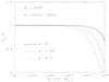	Fig. 8 The ratio bL/b, as in Fig. 7, but as a function of M, at redshifts z = 0,1.25, and 2.5.
In the text

References

- Bardeen, J. M., Bond, J. R., Kaiser, N., & Szalay, A. S. 1986, ApJ, 304, 15 [NASA ADS] [CrossRef] [Google Scholar]
- Blanchard, A., Valls-Gabaud, D., & Mamon, G. A. 1992, A&A, 264, 365 [NASA ADS] [Google Scholar]
- Bond, J. R., Cole, S., Efstathiou, G., & Kaiser, N. 1991, ApJ, 379, 440 [NASA ADS] [CrossRef] [Google Scholar]
- Cole, S., & Kaiser, N. 1989, MNRAS, 237, 1127 [NASA ADS] [Google Scholar]
- Coles, P. 1989, MNRAS, 238, 319 [NASA ADS] [Google Scholar]
- Coles, P., Melott, A. L., & Shandarin, S. F. 1993, MNRAS, 260, 765 [NASA ADS] [Google Scholar]
- Cooray, A., & Sheth, R. 2002, Phys. Rep., 372, 1 [NASA ADS] [CrossRef] [Google Scholar]
- Cuesta, A. J., Prada, F., Klypin, A., & Moles, M. 2008, MNRAS, 389, 385 [NASA ADS] [CrossRef] [Google Scholar]
- Desjacques, V. 2008, Phys. Rev. D, 78, 103503 [NASA ADS] [CrossRef] [Google Scholar]
- Desjacques, V., & Sheth, R. K. 2010, Phys. Rev. D, 81, 023526 [NASA ADS] [CrossRef] [Google Scholar]
- Fry, J. N., & Gaztanaga, E. 1993, ApJ, 413, 447 [NASA ADS] [CrossRef] [Google Scholar]
- Hamana, T., Yoshida, N., Suto, Y., & Evrard, A. E. 2001, ApJ, 561, L143 [NASA ADS] [CrossRef] [Google Scholar]
- Hu, W., & Kravtsov, A. V. 2003, ApJ, 584, 702 [NASA ADS] [CrossRef] [Google Scholar]
- Kaiser, N. 1984, ApJ, 284, L9 [NASA ADS] [CrossRef] [Google Scholar]
- Lumsden, S. L., Heavens, A. F., & Peacock, J. A. 1989, MNRAS, 238, 293 [NASA ADS] [Google Scholar]
- Manera, M., & Gaztanaga, E. 2010 [arXiv:0912.0446] [Google Scholar]
- Manera, M., Sheth, R. K., & Scoccimarro, R. 2010, MNRAS, 402, 589 [NASA ADS] [CrossRef] [Google Scholar]
- McCracken, H. J., Ilbert, O., Mellier, Y., et al., 2008, A&A, 479, 321 [NASA ADS] [CrossRef] [EDP Sciences] [Google Scholar]
- Melott, A. L., Pellman, T. F., & Shandarin, S. F. 1994, MNRAS, 269, 626 [NASA ADS] [Google Scholar]
- Mo, H. J., & White, S. D. M. 1996, MNRAS, 282, 347 [NASA ADS] [CrossRef] [Google Scholar]
- Mo, H. J., Jing, Y. P., & White, S. D. M. 1997, MNRAS, 284, 189 [NASA ADS] [Google Scholar]
- Navarro, J. F., Frenk, C. S., & White, S. D. M. 1997, ApJ, 490, 493 [NASA ADS] [CrossRef] [Google Scholar]
- Padilla, N. D., Baugh, C. M., Eke, V. R., et al. 2004, MNRAS, 352, 211 [NASA ADS] [CrossRef] [Google Scholar]
- Peebles, P. J. E. 1980, The large scale structure of the universe (Princeton: Princeton university press) [Google Scholar]
- Pillepich, A., Porciani, C., & Hahn, O. 2010, MNRAS, 402, 191 [NASA ADS] [CrossRef] [Google Scholar]
- Politzer, H. D., & Wise, M. B. 1984, ApJ, 285, L1 [NASA ADS] [CrossRef] [Google Scholar]
- Press, W., & Schechter, P. 1974, ApJ, 187, 425 [NASA ADS] [CrossRef] [Google Scholar]
- Sheth, R. K., & Tormen, G. 1999, MNRAS, 308, 119 [NASA ADS] [CrossRef] [Google Scholar]
- Sheth, R. K., Mo, H. J., & Tormen, G. 2001, MNRAS, 323, 1 [NASA ADS] [CrossRef] [Google Scholar]
- Tinker, J., Kravtsov, A. V., Klypin, A., et al. 2008, ApJ, 688, 709 [NASA ADS] [CrossRef] [Google Scholar]
- Tinker, J., Robertson, B. E., Kravtsov, A. V. 2010, ApJ, 724, 878 [NASA ADS] [CrossRef] [Google Scholar]
- Valageas, P. 2002, A&A, 382, 450 [NASA ADS] [CrossRef] [EDP Sciences] [Google Scholar]
- Valageas, P. 2009, A&A, 508, 93 [NASA ADS] [CrossRef] [EDP Sciences] [Google Scholar]
- Valageas, P. 2010, A&A, 514, A46 [NASA ADS] [CrossRef] [EDP Sciences] [Google Scholar]
- Zeldovich, Y. B. 1970, A&A, 5, 84 [NASA ADS] [Google Scholar]
- Zheng, Z., & Weinberg, D. H. 2007, ApJ, 659, 1 [NASA ADS] [CrossRef] [Google Scholar]