| Issue |
A&A
Volume 525, January 2011
|
|
|---|---|---|
| Article Number | A116 | |
| Number of page(s) | 9 | |
| Section | Interstellar and circumstellar matter | |
| DOI | https://doi.org/10.1051/0004-6361/201015050 | |
| Published online | 06 December 2010 | |
The tight correlation of CCH and c-C3H2 in diffuse and translucent clouds ⋆
1
LERMA, UMR 8112 du CNRS, Observatoire de Paris, École Normale Supérieure, UPMC
& UCP,
France
e-mail: This email address is being protected from spambots. You need JavaScript enabled to view it.
; This email address is being protected from spambots. You need JavaScript enabled to view it.
; This email address is being protected from spambots. You need JavaScript enabled to view it.
; This email address is being protected from spambots. You need JavaScript enabled to view it.
2
Centre for Astronomy, Nicolaus Copernicus University,
Gagarina 11,
87-100
Toruń,
Poland
e-mail: This email address is being protected from spambots. You need JavaScript enabled to view it.
3
Astronomical Observatory of the Jagiellonian University,
Orla 171,
Kraków,
Poland
e-mail: This email address is being protected from spambots. You need JavaScript enabled to view it.
4
Laboratoire d’Astrophysique de Grenoble, Université Joseph Fourier
and CNRS UMR 5571, Observatoire de Grenoble, France
e-mail: This email address is being protected from spambots. You need JavaScript enabled to view it.
Received:
26
May
2010
Accepted:
27
September
2010
Abstract
Using the IRAM 30 m telescope we observed molecular absorption lines from CCH and c-C3H2 produced by diffuse and translucent clouds along the lines of sight towards massive star forming regions. The same sources are surveyed with Herschel/HIFI as part of the PRISMAS guaranteed time program, for molecular absorption lines due to hydrides and carbon clusters. The background sources are massive star-forming regions (G34.3 + 0.1, G10.62−0.39, W51, W49N) and SgrA ∗ . The line profiles of the CCH and c-C3H2 are strikingly similar for all lines of sight, showing that the ratio of the opacities of the probed transitions, (JKa,Kc = 21,2−10,1) for c-C3H2 and (J = 1−0,F = 5/2−3/2) for CCH, is nearly constant along all lines of sight, at τCCH ~ 1.8 × τc - C3H2. As a consequence, the ratio of the column densities of CCH and c-C3H2 is nearly constant and similar to the value derived earlier for diffuse clouds detected along lines of sight towards extragalactic continuum sources, N(CCH) = (28 ± 1.4)N(c - C3H2) (Lucas & Liszt 2000, A&A, 358, 1069). PDR models are able to reproduce the observed CCH column densities for the range of physical conditions appropriate for the absorbing matter (n = 100−3000 cm-3; AV = 1−5 mag) but can neither fit the observed c-C3H2 column densities nor the tight correlation between CCH and c-C3H2.
Key words: ISM: clouds / ISM: molecules
Based on observations obtained with the IRAM 30 m telescope.
© ESO, 2010
1. Introduction
Small carbon containing molecules, with a total of about 1 to 3 carbon atoms, have several
interesting properties: they are ubiquitous in the interstellar medium, they are key actors
in the formation of long carbon chains and other hydrocarbons, and they are involved in
photo-fragmentation process of larger species like PAHs. Of particular interest is the
sputtering of carbonaceous nanoparticules, which form a likely source for the high abundance
of hydrocarbon molecules detected in the ISM (Pety et al. 2005). It is widely believed that carbon-chain or ring species with more atoms
than species detected by radio telescopes might be the candidates for the diffuse
interstellar bands (Douglas 1977; Herbig 1975; Herbig 1995). Laboratory studies of the fragmentation process of PAHs have provided further
support to this conjecture (Tielens 2008;
Useli-Bacchitta & Joblin 2007), but no
definitive proof yet. The carbon chemistry is particularly complex. It is initiated in the
gas phase by the slow radiative association of ionized carbon with molecular hydrogen
leading to  since the direct
formation of CH+ has a high endothermicity of over 4000 K (see the discussion in
Godard et al. 2009, and references therein).
then rapidly reacts
with H2, leading to
since the direct
formation of CH+ has a high endothermicity of over 4000 K (see the discussion in
Godard et al. 2009, and references therein).
then rapidly reacts
with H2, leading to  which acts as
the seed for most of the interstellar hydrocarbons (e.g. CH, C2H2), as
well as the carbon clusters C2 and C3. Comparison of carbon clusters
and carbon hydrides abundances is therefore an excellent test of the chemical paths to the
carbon chemistry and, more generally, to the buildup of molecular complexity in the
ISM.
which acts as
the seed for most of the interstellar hydrocarbons (e.g. CH, C2H2), as
well as the carbon clusters C2 and C3. Comparison of carbon clusters
and carbon hydrides abundances is therefore an excellent test of the chemical paths to the
carbon chemistry and, more generally, to the buildup of molecular complexity in the
ISM.
Characteristics of the observed sources.
Spectroscopic parameters for the observed species.
The interstellar ethynyl radical (CCH) was discovered in 1974 by Tucker et al. (1974). It was identified by its radio-astronomical
spectra, with the help of its four intense hyperfine components, before laboratory
spectroscopy of gaseous CCH was performed. In the interstellar medium, CCH is thought to
result from the photodissociation of acetylene (C2H2) and from the
dissociative recombination of  and
and
 (Mul &
McGowan 1980). The neutral-neutral reaction between C and CH2 also contributes to
forming CCH especially in moderately shielded regions. This route has been confirmed by the
recent measurements of Sakai et al. (2010), who
obtained different abundances for the two isotopologues C13CH and
13CCH. Since the two carbon atoms play equivalent roles in the photodissociation
of acetylene and in the dissociative recombination of
(Mul &
McGowan 1980). The neutral-neutral reaction between C and CH2 also contributes to
forming CCH especially in moderately shielded regions. This route has been confirmed by the
recent measurements of Sakai et al. (2010), who
obtained different abundances for the two isotopologues C13CH and
13CCH. Since the two carbon atoms play equivalent roles in the photodissociation
of acetylene and in the dissociative recombination of
 and
, the reaction
between C and CH2 is the sole CCH formation mechanism that can produce such a
difference in the C13CH and 13CCH abundances because the two carbon
atoms have different origins.
and
, the reaction
between C and CH2 is the sole CCH formation mechanism that can produce such a
difference in the C13CH and 13CCH abundances because the two carbon
atoms have different origins.
Cyclopropenylidene (c-C3H2) is the first hydrocarbon ring detected in
space. It was reported by Thaddeus et al. (1985);
c-C3H2 lines were detected as early as 1981 (Thaddeus et al.) but
were not identified as a cyclopropenylidene until 1985. c-C3H2 is also
one of the most abundant molecules with 3 carbon atoms in the interstellar medium (Teyssier
et al. 2004). Its main gas phase formation route is
the dissociative recombination of
c-C3 .
.
Both CCH and c-C3H2 are therefore good probes for hydrocarbons in the diffuse interstellar medium, especially carbon chains and radicals. While the inventory of gas-phase carbon molecules with two or three C-atoms is fairly complete (Marcelino et al. 2007), knowledge of species with more carbon atoms is still fragmentary. Combined measurements of CCH and c-C3H2 can shed light on the chemical processes leading to larger hydrocarbons. Lucas & Liszt (2000) show that interstellar absorption features from CCH and c-C3H2 are correlated well in the millimeter spectra of extragalactic background radio sources with N(CCH)/N(c-C3H2) = 27.7 ± 8. Pety et al. (2005) found a spatial correlation of emission maps of the edge of the Horsehead nebula, with a strong similarity between maps of CCH, c-C3H2 and C4H, but with differences in the mean abundance ratios: N(CCH)/N(c-C3H2) = ~12 and N(CCH)/N(C4H) = ~7.
In this paper, we present new absorption spectra, sampling the diffuse and translucent matter in the Galactic Plane, along lines of sight towards bright millimeter continuum sources. The data set belongs to complementary absorption spectroscopy data obtained with the IRAM-30 m telescope towards the targets of the PRISMAS (PRobing InterStellar Molecules with Absorption line Studies) Herschel key program. This project aims at probing the first steps of the oxygen, carbon and nitrogen chemistry in the diffuse interstellar medium. Extensive spectroscopic studies of key interstellar molecules not easily accessible at other wavelengths, namely hydrides and carbon clusters, are currently performed by Herschel/HIFI. The target sources have been selected as strong (sub)millimeter continuum sources, with known intervening interstellar features along the lines of sight. The same sources can be observed at millimeter wavelengths, although the continuum emission is produced by the embedded HII regions rather than by dust. While a first set of observations, covering HCO+, HCN, HNC and CN spectra, has been presented by Godard et al. (2010), the data relative to the hydrocarbon chemistry are presented in this paper. The analyzed objects are listed in Table 1. Table 1 also lists their distances from Fish et al. (2003).
The next section describes the IRAM-30 m observations. The results are presented in Sect. 3; a comparison with PDR models is given in Sect. 4, while Sect. 5 presents the conclusions.
2. Observations
2.1. Data analysis and processing
The observations were performed with the IRAM-30 m telescope in 2006 August and December. We used the A100 and B100 receivers, simultaneously with either the A230, B230 or the C150, D150 receivers. All receivers were operated in single side band mode, with a rejection of the image side band better than a factor of 20 (13dB). The observations were performed with the wobbling secondary reflector to obtain flat and stable baselines, and an accurate measurement of the 3 mm radio continuum intensity. The wobbler throw was 240 arcsec and the switching rate 0.5 Hz. The weather conditions were averaged with 5−10 mm of water vapor in August 2006 and less than 3 mm in December 2006. The pointing was checked on nearby planets and continuum sources, and was found accurate within 5 arcsec. The lines were analyzed with the flexible, high spectral resolution backend VESPA, tuned to a spectral resolution of 40 kHz (~0.13 km s-1), and spectral bandpass of 120 MHz covering a velocity range of ~400 km s-1. We also used the 1 MHz filterbank to obtain broad band spectra. We searched for the ground state transition of CCH at 87.316 GHz and the 21,2−10,1 transition of ortho c-C3H2 at 85.338 GHz. The J = 2–1 line of HCS+ was observed simultaneously with c-C3H2 as their frequencies are very close (the velocity shift is −31.6 km s-1). The spectroscopic parameters of the observed molecular transitions are listed in Table 2. The IRAM-30 m spectra are shown in Fig. 1.
The data processing was done with the GILDAS1
softwares (e.g. Pety 2005). The IRAM-30 m data
were first calibrated to the  scale using
the chopper wheel method (Penzias & Burrus 1973), and finally converted to main beam temperatures
Tmb using the forward and main beam efficiencies
Feff and Beff appropriate for 85
and 87 GHz: Feff = 0.95 and
Beff = 0.75. The resulting temperature accuracy is
~10%, as checked by the variation of the intensity of the strong CCH emission
lines in the spectra between different days.
scale using
the chopper wheel method (Penzias & Burrus 1973), and finally converted to main beam temperatures
Tmb using the forward and main beam efficiencies
Feff and Beff appropriate for 85
and 87 GHz: Feff = 0.95 and
Beff = 0.75. The resulting temperature accuracy is
~10%, as checked by the variation of the intensity of the strong CCH emission
lines in the spectra between different days.
The spectra show strong emission lines associated with the massive cores surrounding the compact HII regions, together with absorption lines from the foreground matter along the line of sight. In the massive star forming regions, the continuum emission is mainly free-free emission while we detect the non thermal millimeter continuum emission from SgrA∗. The continuum intensities are listed in Table 1. Except for SgrA∗, emission lines of CCH (13/2,2−01/2,1) at 87.316 GHz, CCH (13/2,1−01/2,0) at 87.328 GHz, and c-C3H2 21,2−10,1 at 85.339 GHz are detected at the velocities of the background sources. The J = 2–1 line of HCS+ at 85.347 GHz i.e. −31.6 km s-1 relative to the c-C3H2 (21,2−10,1) line is also detected in all sources. Emission lines have close to Gaussian profiles towards G10.6–0.39, G34.3+0.15 and W51, while they are clearly double peaked towards W49N, a feature also seen in other molecular lines Williams et al. (2004). In this paper, we analyse the absorption produced by the foreground matter along the line of sight and will not comment further on the emission spectra.
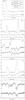 |
Fig. 1 Spectra obtained with the IRAM-30 m telescope. The velocity scale is given relative to the Local Standard of Rest (LSR). The spectra have been normalized by dividing the individual measurements by the source continuum intensities. The CCH spectra have been offset for clarity. Except for G10.6, the two strongest CCH hyperfine components at 87.317 and 87.329 GHz are shown. The emission line shifted by −31.6 km s-1 from c-C3H2 is the HCS+J = 2–1 transition at 85.347 GHz. An inset showing the velocities of the absorption features is presented for G10.62. |
 (1)and
hence:
(1)and
hence:  (2)The CCH and
c-C3H2 absorption profiles are strikingly similar, with narrow
components superposed with broad and shallow features. Given the complexity of these
profiles, we did not attempt to fit them entirely but preferred to restrict the analysis
to the narrow features that have Gaussian profiles and are easily identified in the
spectra (Fig. 2). We started with the CCH data that
have the best S/N ratio. As the main CCH hyperfine
components is separated from the nearest satellite line by ~11.7 MHz
~40 km s-1, the absorptions caused by these components do not
overlap in most cases. We used the detection of the main and satellite lines to check the
quality of the fit of the line parameters. Once the fit of the CCH spectra was
satisfactory, and in order to decrease the number of free parameters in the fit, we used
the centroid velocities of the CCH velocity components as constraints for the fit of the
c-C3H2 line profiles. The high spectral resolution used in this
study allowed us to separate velocity components which were blended in previous studies
(Madden et al. 1989; Cernicharo et al. 1999; Cox et al. 1988). The global analysis of the CCH and c-C3H2
absorption profiles (Fig. 4) shows that the broad
absorption features have similar properties to the narrow lines.
(2)The CCH and
c-C3H2 absorption profiles are strikingly similar, with narrow
components superposed with broad and shallow features. Given the complexity of these
profiles, we did not attempt to fit them entirely but preferred to restrict the analysis
to the narrow features that have Gaussian profiles and are easily identified in the
spectra (Fig. 2). We started with the CCH data that
have the best S/N ratio. As the main CCH hyperfine
components is separated from the nearest satellite line by ~11.7 MHz
~40 km s-1, the absorptions caused by these components do not
overlap in most cases. We used the detection of the main and satellite lines to check the
quality of the fit of the line parameters. Once the fit of the CCH spectra was
satisfactory, and in order to decrease the number of free parameters in the fit, we used
the centroid velocities of the CCH velocity components as constraints for the fit of the
c-C3H2 line profiles. The high spectral resolution used in this
study allowed us to separate velocity components which were blended in previous studies
(Madden et al. 1989; Cernicharo et al. 1999; Cox et al. 1988). The global analysis of the CCH and c-C3H2
absorption profiles (Fig. 4) shows that the broad
absorption features have similar properties to the narrow lines.
Although the available HI data (Fish et al. 2003; Koo 1997) have a lower spectral resolution than the data presented here, there is a generally good correspondence of the velocity ranges where absorption is detected in HI and in other molecules such as HCO+ or CCH. Note however that some HI features seem to have little molecular counterpart while the reverse is never seen. As discussed further in (Godard et al. 2010; Neufeld et al. 2010b), the opacities of the absorption features do not scale with the HI opacities, indicating that the abundances of the different species relative to HI vary among velocity components. The recent Herschel-HIFI spectra obtained within the framework of the PRISMAS key programme show more extensive examples of molecular line profiles towards G10.6, W49N and W51 (Falgarone et al. 2010; Gerin et al. 2010a,b; Neufeld et al. 2010a,b; Sonnentrucker et al. 2010; Persson et al. 2010). The Herschel data revealed that absorption features from the molecular ions CH+, OH+ and H2O+, and from the HF molecule are better correlated with HI than those from triatomic molecules such as CCH and HCO+ (Falgarone et al. 2010; Gerin et al. 2010a; Neufeld et al. 2010a,b; Sonnentrucker et al. 2010).
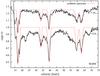 |
Fig. 2 The multiple velocity component fit overlayed on a zoom of the W49N data. Broad absorption is clearly detected in CCH and c-C3H2 in the velocity ranges ~30−45 and ~50−70 km s-1corresponding to the Sagittarius and Scutum spiral arms. |
2.2. Derivation of CCH column densities
We analyzed the main CCH hyperfine component at 87.316 GHz. As shown in Fig. 1, the absorption spectra are not saturated, for all hyperfine components, including the strongest one. Furthermore, the satellite hyperfine components that have lower relative intensities (Table 2) present weaker absorption features than the strongest component. For all sources, the ratio of the opacities of the satellite line at 87.328 GHz divided by the opacity of the main line at 87.317 GHz is equal to 0.5, the ratio of the relative intensities, as expected for unsaturated lines. This shows that the opacity of the absorption features is truly moderate, and does not result from partial coverage of the background source of saturated absorption lines, because in the latter case, we would expect that the relative intensities of the CCH hyperfine components would depart from their theoretical values, that are listed in Table 2. At millimeter wavelengths, the covering factor of the absorbing matter is close to unity.
We derived the molecule column densities using the relation:
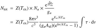 (3)where
Z(Tex) is the partition function computed
at the excitation temperature Tex,
Ntot and Nu are
the total column density and the column density in the upper state of the transition
respectively, gu is the statistical weight of
the upper level, Aul is the Einstein coefficient for
spontaneous emission, ν is the line frequency and
∫τ·dv is the line opacity integrated over
the line profile. For molecules with hyperfine structure like CCH it can be easier to
compute the column density without taking the hyperfine structure into account, provided
that the correct line opacity, i.e. the sum of the opacities of all hyperfine components,
is used. Following the latter approach and assuming that the excitation temperature is
equal to the CMB, 2.73 K, i.e. collisional excitation is negligible because of the low gas
density and moderate kinetic temperature, this leads to the relation given by Lucas
& Liszt (2000):
(3)where
Z(Tex) is the partition function computed
at the excitation temperature Tex,
Ntot and Nu are
the total column density and the column density in the upper state of the transition
respectively, gu is the statistical weight of
the upper level, Aul is the Einstein coefficient for
spontaneous emission, ν is the line frequency and
∫τ·dv is the line opacity integrated over
the line profile. For molecules with hyperfine structure like CCH it can be easier to
compute the column density without taking the hyperfine structure into account, provided
that the correct line opacity, i.e. the sum of the opacities of all hyperfine components,
is used. Following the latter approach and assuming that the excitation temperature is
equal to the CMB, 2.73 K, i.e. collisional excitation is negligible because of the low gas
density and moderate kinetic temperature, this leads to the relation given by Lucas
& Liszt (2000):
![Mathematical equation: \begin{eqnarray} N(C_2H) & = & 2.71 \times 10^{13} \cdot 2.4 \cdot \int \tau {\rm d}v \ [{\rm cm}^{-2}] \nonumber \\ & = & (2.4 \cdot 2.71 \cdot 1.065) \times 10^{13} \cdot fwhm \cdot \tau \rm [cm^{-2}] \end{eqnarray}](/articles/aa/full_html/2011/01/aa15050-10/aa15050-10-eq95.png) (4)where
fwhm is the line full width at half maximum in km s-1
and τ is the opacity of the main hyperfine component
(13/2,2−01/2,1 at 87.316 GHz). The factor 2.4 corrects for
the opacities of the satellite lines because Lucas & Liszt (2000) quoted this formula differently, with the sum of the opacities of
all hyperfine components rather the opacity of the main component
(13/2,2−01/2,1) we are using. For a Gaussian line profile
the integrated line opacity is proportional to the product of the line width at half
maximum fwhm and central opacity τ. The factor is very
close to unity, and can be written as
(4)where
fwhm is the line full width at half maximum in km s-1
and τ is the opacity of the main hyperfine component
(13/2,2−01/2,1 at 87.316 GHz). The factor 2.4 corrects for
the opacities of the satellite lines because Lucas & Liszt (2000) quoted this formula differently, with the sum of the opacities of
all hyperfine components rather the opacity of the main component
(13/2,2−01/2,1) we are using. For a Gaussian line profile
the integrated line opacity is proportional to the product of the line width at half
maximum fwhm and central opacity τ. The factor is very
close to unity, and can be written as  .
.
The hypothesis of negligible collisional excitation has been confirmed by the multi transition analysis of the HCO+ profiles (Godard et al. 2010) and by additional, non LTE, statistical equilibrium calculations performed with the RADEX software (van der Tak et al. 2007, Black private communication). We checked that the excitation temperature of the observed CCH transition stays below 3 K, for most of the domain of physical conditions applicable to the line of sight clouds: the absorption features are formed in moderately dense gas: n(H2) = 100–3000 cm-3 (Plume et al. 2004; Vastel et al. 2000; Godard et al. 2010). These analyses have shown that, with such physical conditions, the collisional excitation of polar molecules is rather ineffective, and the excitation temperature remains close to the cosmic background temperature. The excitation temperature starts to depart significantly from the cosmic background temperature at the highest densities (n(H2) > 3000 cm-3), but never rises above 5 K. Therefore, we can confidently derive the molecular column densities assuming that the excitation temperature is equal to the CMB.
2.3. Derivation of c-C3H2 column densities
Absorption in the strong 212−101 transition of ortho c-C3H2 at 85.338 GHz is detected in all sources. The similarity of the spectra to those of CCH (Fig. 4) suggests that the absorption features are not saturated and that we can derive accurate column densities from the measured line opacities.
The c-C3H2 column densities were derived from the relation of
Lucas & Liszt (2000):
![Mathematical equation: \begin{equation} N(c-C_3H_2) = 4.36 \cdot 10^{12} \cdot fwhm \cdot \tau \ \rm [cm^{-2}]. \end{equation}](/articles/aa/full_html/2011/01/aa15050-10/aa15050-10-eq103.png) (5)As for CCH, this
equation is based on the assumption of no collisional excitation. The results are listed
in Table 3.
(5)As for CCH, this
equation is based on the assumption of no collisional excitation. The results are listed
in Table 3.
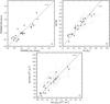 |
Fig. 3 a) Comparison of the Full Width at Half Maximum (FWHM) of the velocity components identified in the CCH and c-C3H2 line profiles. The straight line indicates a slope of 1. b) Comparison of the line center opacities τ of the observed CCH and c-C3H2 lines. For CCH the opacity of the strongest hyperfine component at 87.317 GHz is plotted. The line shows the mean relation with a slope of a = 1.8. c) Comparison of the column densities of CCH and c-C3H2. The line shows a slope of 2.8, corresponding to the relation obtained by Lucas & Liszt (2000) towards diffuse clouds at high Galactic latitude, N(CCH) ~ 28 N(c-C3H2). We get a similar result, N(CCH)/N(c-C3H2) = 28.2 ± 1.4. |
2.4. HCS+
The HCS+J = 2−1 transition at 85.347 GHz is detected in emission, shifted by −31.6 km s-1 from c-C3H2 line at 85.338 GHz, but does not show any detectable absorption down to the noise level. Assuming Tex = 2.73 K, we derived an upper limit of τ ≤ 0.1 and N(HCS+) = 9.27 × 10¹²fwhm·τ < 9.3 × 1011 cm-2 for a line width of 1 km s-1.
3. Results
Table 3 summarizes the derived CCH and c-C3H2 line parameters and column densities. For each velocity component, the full line width at half maximum (fwhm), the opacity (τ) and column density (N) are given. The distance to the different velocity components is also listed. It is derived assuming a flat rotation curve using: θ0 = 220 km s-1 and R0 = 8.5 kpc as recommended by the IAU (Kerr & Lynden-Bell 1986).
3.1. Analysis of CCH and c-C3H2 line profiles
Results of measurements for absorption structures of CCH and c-C3H2 (the full width at half maximum fwhm, the line center opacity τ, the column density N).
As shown in Fig. 1, the CCH and c-C3H2 spectra are strikingly similar. To be more quantitative, we show in Figs. 3a and 3b comparisons of the line full width at half maximum fwhm and central opacity τ for the analyzed absorption features. The correlation coefficients for the derived central opacity and line width are 0.85 and 0.89 respectively, showing that these variable are strongly correlated. Figure 4 presents direct comparisons of the line profiles expressed in opacity units, for the entire velocity ranges where absorption is detected. The symbols indicate the different sources. The five sources share the same mean relation.
We therefore conclude that the data are consistent with the hypothesis that the CCH and c-C3H2 absorption features have identical line widths, and that their line opacities are proportional with τ(CCH) = 1.8 ± 0.2·τ(c - C3H2), where τ(CCH) refers to the opacity of the main hyperfine component. This conclusion is based on the sole analysis of the line profiles and does not depend on any assumption on the line formation mechanism, nor on the decomposition method of the complex profiles into individual velocity components.
3.2. Comparison of CCH and c-C3H2 column densities
As expected from the tight relationship of the CCH and c-C3H2 line opacities and line widths, column densities of CCH and c-C3H2 are linearly correlated, with a correlation coefficient of 0.88. Fig. 3c) illustrates this correlation. It is interesting to note that we obtained a very similar relationship between the CCH and c-C3H2 column densities as in the study of local diffuse clouds performed by Lucas & Liszt (2000): N(CCH)/N(c - C3H2) = 28.2 ± 1.4 while they found N(CCH)/N(CthHtw) = 27.7 ± 8.
4. Chemistry
We used the Meudon-PDR code (Le Petit et al. 2006;
Goicoechea & Le Bourlot 2007; González-García
et al. 2008) to investigate the production mechanisms
of CCH and c-C3H2. The cold gas is modeled as a slab of either
constant density or constant pressure, illuminated by the average interstellar radiation
field on both sides. The code assumes that the chemistry has reached steady state, and
computes the thermal equilibrium by balancing the cooling and heating rates at each point in
the slab. The main input parameters are listed in Table 4. We used the default values for the elemental abundances, extinction curve and
cosmic ray ionization rate ζ as discussed by e.g. (Le Petit et al. 2006). The physical conditions of the matter giving rise
to the absorption features are fairly well known from previous works: the gas densities and
total extinction across each absorption feature are low to moderate (Godard et al. 2010; Gerin et al. 2010b). We therefore chose to run models with constant gas densities ranging
from 100 to 1000 cm-3, and added two models with constant pressure. We show
models with total hydrogen densities of n(H) = 100, 250, 500, 750 and
1000 cm-3, gas pressures of 3500 and 104 K cm-3, and
total extinction across the slab of AV = 1,3, and 5 mag. For
all models, the radiation field has been set to the mean interstellar radiation field in the
solar neighborhood G0 = 1. We briefly explored the role of the
cosmic ray ionization rate ζ, by running models with
ζ = 10-16 s-1 and
2 × 10-16 s-1 for
nH = 500 cm-3, following the recent
H observations summarized in Indriolo et al. (2007)
that suggest that ζ may be higher in the diffuse interstellar medium than
in the dense gas. Table 5 lists the model predictions
for the column densities across the slab.
observations summarized in Indriolo et al. (2007)
that suggest that ζ may be higher in the diffuse interstellar medium than
in the dense gas. Table 5 lists the model predictions
for the column densities across the slab.
Figure 5 shows the predicted column densities of C+, C, CO, CH, CCH and c-C3H2 across the slab for the models. The constant density models are plotted with squares, while the constant pressure models are indicated by stars. Models with AV = 3 mag are shown with black symbols and full lines, while we show models with AV = 5 mag with white symbols and dotted lines and models with AV = 1 mag with crosses. To ease the comparison, we scaled all model predictions to AV = 3 mag. The predicted column densities of the AV = 5 mag cases are therefore multiplied by 0.6, while the predicted column densities of the AV = 1 mag are multiplied by 3. The constant pressure models are plotted using the maximum density as abscissa.
In these models, CCH reaches total column densities ranging from comparable to somewhat higher than what we measured, while the c-C3H2 column densities remain lower than observed. The abundance ratio ranges from ~160 to >400, the highest value being obtained for the lowest density models. The spatial distribution of the CCH and c-C3H2 abundances is also different: while CCH is present as soon as Av > 0.5 mag or even at lower extinctions for the n = 1000 cm-3 models, c-C3H2 is confined in the inner core of the slab with Av > 1 mag. The behaviors of the predicted CCH and c-C3H2 column densities with the slab density and total extinction also differ. Except for the densities in the AV = 1 mag case, the predicted CCH column density is independent of the model density and scales with AV. On the contrary, the highest c-C3H2 column densities are obtained for the models with highest extinction, and at a given extinction for the highest density.
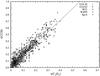 |
Fig. 4 Comparison of the opacities of the individual velocity channels for the CCH (15/2,5/2−03/2,3/2) and c-C3H2 (21,2−10,1) lines. The straight line shows the mean ratio τ(CCH)/τ(c-C3H2) = 1.8. The typical error on the opacities in each velocity channel is about ~0.1. |
All models predict a high molecular fraction 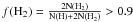 , since atomic hydrogen is only
dominant over molecular hydrogen in the most external layers
(AV < 0.1 mag) of the modeled clouds. The molecular
fraction is not known for all lines of sight. For G10.6–0.4 and W49N, it is possible to
estimate this parameter from the comparison of the total extinction along the line of sight
with the observed HI absorption. The average molecular fraction is 0.4−0.6 (Godard et al.
2010; Neufeld et al. 2010a) but the detailed comparison of the HI and molecular absorption
profiles reveals that a variety of conditions is present, from very diffuse phases with
mostly atomic gas to mostly molecular gas (Neufeld et al. 2010b).
, since atomic hydrogen is only
dominant over molecular hydrogen in the most external layers
(AV < 0.1 mag) of the modeled clouds. The molecular
fraction is not known for all lines of sight. For G10.6–0.4 and W49N, it is possible to
estimate this parameter from the comparison of the total extinction along the line of sight
with the observed HI absorption. The average molecular fraction is 0.4−0.6 (Godard et al.
2010; Neufeld et al. 2010a) but the detailed comparison of the HI and molecular absorption
profiles reveals that a variety of conditions is present, from very diffuse phases with
mostly atomic gas to mostly molecular gas (Neufeld et al. 2010b).
Figure 6 presents abundances relative to H2 derived from the PDR models in the sampled parameter space. Because both CH and CCH scale well with the extinction across the slab, their abundances relative to H2 show little variation with the gas density. The PDR models reproduce the well known correlation of CH with molecular hydrogen (Sheffer et al. 2008, and references therein). The predicted abundances are slightly higher than the mean CH abundance derived from visible absorption spectroscopy: we deduce [CH] ~ 1.3 ± 0.2 × 10⁻⁷ and [CCH] ~ 7.0 ± 1.5 × 10⁻⁸ relative to the H2 column density, while Sheffer et al. (2008) derived [CH] = 3.6 × 10⁻⁸ for diffuse and translucent clouds of somewhat lower total extinctions. It is remarkable that, for both CH and CCH, the variation of their abundance relative to H2 does not exceed 20% for most of the studied models.
Parameters of the PDR models
The PDR models also predict that the ratio of the CH and CCH abundances is well defined:
N(CH)/N(CCH) = 1.8 ± 0.3. This close association of CH
and CCH is confirmed when looking at the spatial gradients of the CH and CCH densities in a
single slab as the spatial variations of CH and CCH are very similar. This behavior can be
understood since these species are closely chemically related. CCH is produced by the
photodissociation of acetylene (Roberge et al. 1991)
and by the reaction of atomic carbon with CH2 (Smith et al. 2004; Sakai et al. 2010). The
dissociative recombination of molecular ions such as C2H2+
and C2H3+ also plays a role. CCH is destroyed by
photodissociation and by reaction with ionized and atomic carbon, initiating the formation
of polyynes. As the carbon chemistry is initiated by the radiative association between
C+ and H2 producing (Black
& Dalgarno 1973), it is expected that CH
scales with H2. The formation of diatomic hydrocarbons is relatively easy once
is formed because the
reactions with C+ and C are rapid. Hence models predict that CH and CCH reside
in the same environment. Furthermore, the predicted CH2 column densities are
similar to those of CH and slightly higher than those of CCH, with a trend with the gas
density. CH is more abundant for the low densities, while CH2 becomes dominant
for n ≥ 500 cm-3.
Within the limited parameter space sampled, we did not find any strong variation of the predicted CCH or CH abundances with the cosmic ray ionization rate ζ. We recovered the known decrease of the CO abundance with increasing ζ (see Table 5 and Fig. 6).
It will be interesting to confirm these model predictions by observing CH along the same lines of sight as CCH. Observations of the ground state rotational lines of CH at 532 and 536 GHz at high spectral resolution are now feasible using the HIFI instrument on board the Herschel Space Observatory. First observations presented by (Gerin et al. 2010b) show a tight association of CH and CCH for a limited source sample. If the trend is confirmed, it will be possible to use CCH as a proxy for molecular hydrogen in diffuse and translucent gas, since CH has been shown to be tightly correlated with the molecular hydrogen (Federman 1982; Liszt & Lucas 2002; Weselak et al. 2004; Sheffer et al. 2008).
Column densities N[cm-2] predicted by the PDR models. Models 1–15 and 18–21 are isochoric (constant nH) models 16 and 17 are isobaric.
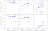 |
Fig. 5 Prediction of the column densities of C+, C, CO, CH, CCH and c-C3H2 from the PDR Meudon models with various hydrogen densities and pressures. The constant density models are plotted with squares while the constant pressure models are shown with stars. These models correspond to AV = 3 mag. Results from models with AV = 5 mag are scaled by 0.6 to compensate for the higher total gas content, they are shown with open squares and dotted lines. Results from models with AV = 1 mag are scaled by 3 to compensate for the lower total gas content, they are shown with crosses. The constant pressure models are plotted using the highest density point as abscissa. |
 |
Fig. 6 Prediction of the abundances relative to H2 of C+, C, CO, CH, CCH and c-C3H2 from the PDR Meudon models with various hydrogen densities and pressures. Models with AV = 5 mag are plotted with open squares, AV = 3 mag with black squares and AV = 1 mag with crosses. Constant pressure models are plotted using the highest density point as abscissa. Models with elevated cosmic ray ionization fluxes are drawn in red, using larger symbols. The gray bars indicate the observed abundances of CH (Sheffer et al. 2008), CCH (Gerin et al. 2010) and c-C3H2(this work, using the scaling with CCH). |
On the contrary, the model does not reproduce the observed properties of c-C3H2 : i) the predicted column densities are lower than the observed column densities; ii) the predicted column density does not scale with the total extinction across the slab. Moreover, because CCH is present across most of the slab, while c-C3H2 is confined to the inner regions, the resulting line profiles are expected to bear the signature of these different environments, with c-C3H2 profiles sampling quieter regions with smaller velocity dispersions than CCH. Therefore a loose correlation between the CCH and c-C3H2 line profiles would be expected based on the PDR model predictions, that contrasts with the observed tight correlation. In the PDR model, c-C3H2 is formed by the dissociative recombination of c-C3H3+ and by the reaction of C with acetylene. It is destroyed by photodissociation and by reactions with atomic carbon. It is likely that other formation mechanisms, yet to be identified, participate to the production of c-C3H2.
The tight correlation of CCH and c-C3H2 was recognized earlier by Lucas & Liszt (2000) and Pety et al. (2005) in different environments (diffuse clouds for the former case and the Horsehead nebula for the latter). The modeling attempts, using an earlier version of the Meudon-PDR code, failed to reproduce this correlation in the context of the Horsehead nebula, a dense molecular cloud illuminated by a moderately intense radiation field (Pety et al. 2005). These authors put forward the hypothesis that the production of c-C3H2 and other carbon radicals is increased by the destruction of very small carbon grains and/or PAHs in the intense FUV radiation field at the surface of the molecular cloud, directly exposed to the radiation from massive stars. In diffuse or translucent clouds, the same mechanism could operate. This scenario needs to be fully tested by including the PAH chemistry in the PDR models.
Godard et al. (2009) have explored the impact of the dissipation of turbulence on the chemistry of diffuse interstellar clouds. They show that the chemical abundances of some molecular species, notably HCO+ and CH+, are significantly modified and become in a much better agreement with observations than the predictions obtained by steady-state PDR models. Their chemical network includes CCH but not c-C3H2. Models with a more extensive chemical network are currently under investigation, to search whether c-C3H2 could be partially produced in the dissipation regions of the interstellar turbulence.
5. Conclusion
We confirm that the tight correlation of CCH and c-C3H2 first established by Lucas & Liszt (2000) towards high latitude diffuse clouds is present in the diffuse and translucent matter along the line of sight towards distant massive star forming regions, with N(CCH) = (28.2 ± 1.4)N(c-C3H2). This correlation confirms the finding by Lucas & Liszt (2000) and extends it to the more distant interstellar matter in the Galactic Plane. While PDR models seem to reproduce the observed properties of CCH, they fail by at least one order of magnitude for c-C3H2. We suggest that CCH might be used as a complementary tracer of molecular hydrogen in diffuse and translucent matter, that can replace CH in environments where no visible spectroscopy can be performed. The HIFI instrument on board the Herschel Space Observatory is now capable of detecting the submillimeter transitions of CH with high accuracy, enabling the direct comparison of CH and CCH.
See http://www.iram.fr/IRAMFR/GILDAS
Acknowledgments
The work was carried out within the framework of the European Associated Laboratory “Astrophysics Poland-France” and also was supported by the Science and High Education Ministry of Poland, grants N203 39/3334. We thank the anonymous referee for her/his very interesting comments that helped to improve the paper.
References
- Black, J. H., & Dalgarno, A. 1973, ApL, 15, 79 [Google Scholar]
- Cernicharo, J., Cox, P., Fossé, D., & Güsten, R. 1999, A&A, 351, 341 [NASA ADS] [Google Scholar]
- Cox, P., Güsten, R., & Henkel, C. 1988, A&A, 206, 108 [NASA ADS] [Google Scholar]
- Douglas, A. E. 1977, Nature, 269, 130 [NASA ADS] [CrossRef] [Google Scholar]
- Falgarone, E., Godard, B., & Cernicharo, J., et al. 2010, A&A, 521, L15 [NASA ADS] [CrossRef] [EDP Sciences] [Google Scholar]
- Federman, S. R. 1982, ApJ, 257, 125 [NASA ADS] [CrossRef] [Google Scholar]
- Fish, V. L., Reid, M. J., Wilner, D. J., & Churchwell, E. 2003, ApJ, 587, 701 [NASA ADS] [CrossRef] [Google Scholar]
- Gerin, M., de Luca, M., Black, J., et al. 2010a, A&A, 518, L110 [NASA ADS] [CrossRef] [EDP Sciences] [Google Scholar]
- Gerin, M., De Luca, M., Goicoechea, J. R., et al. 2010b, A&A, 521, L16 [Google Scholar]
- Godard, B., Falgarone, E., & Pineau des Forêts, G. 2009, A&A, 495, 847 [NASA ADS] [CrossRef] [EDP Sciences] [Google Scholar]
- Godard, B., Falgarone, E., Gerin, M., et al. 2010, A&A, 520, A20 [NASA ADS] [CrossRef] [EDP Sciences] [Google Scholar]
- Goicoechea, J. R., & Le Bourlot, J. 2007, A&A, 467, 1 [NASA ADS] [CrossRef] [EDP Sciences] [Google Scholar]
- González-García, M., Le Bourlot, J., Le Petit, F., & Roueff, E. 2008, A&A, 485, 127 [NASA ADS] [CrossRef] [EDP Sciences] [Google Scholar]
- Herbig, G. H. 1975, ApJ, 196, 129 [NASA ADS] [CrossRef] [Google Scholar]
- Herbig, G. H. 1995, ARA&A, 33, 19 [NASA ADS] [CrossRef] [Google Scholar]
- Indriolo, N., Geballe, T. R., Oka, T., & McCall, B. J. 2007, ApJ, 671, 1736 [NASA ADS] [CrossRef] [Google Scholar]
- Kerr, F. J., & Lynden-Bell, D. 1986, MNRAS, 221, 1023 [NASA ADS] [CrossRef] [Google Scholar]
- Koo, Bon-Chul 1997, ApJS, 108, 489 [NASA ADS] [CrossRef] [Google Scholar]
- Le Petit, F., Nehmé, C., Le Bourlot, J., & Roueff, E. 2006, ApJS, 64, 506 [NASA ADS] [CrossRef] [EDP Sciences] [Google Scholar]
- Liszt, H., & Lucas, R. 2002, A&A, 391, 693 [NASA ADS] [CrossRef] [EDP Sciences] [Google Scholar]
- Lucas, R., & Liszt, H. S. 2000, A&A, 358, 1069 [NASA ADS] [Google Scholar]
- Madden, S. C., Irvine, W. M., Swade, D. A., Matthews, H. E., & Friberg, P. 1989, AJ, 97, 1403 [NASA ADS] [CrossRef] [PubMed] [Google Scholar]
- Marcelino, N., Cernicharo, J., Agũndez, M., et al. 2007, ApJ, 665, L127 [NASA ADS] [CrossRef] [Google Scholar]
- Mul, P. M., & McGowan, J. W. 1980, ApJ, 237, 749 [NASA ADS] [CrossRef] [Google Scholar]
- Müller, H. S. P., Thorwirth, S., Roth, D. A., & Winnewisser, W. 2001, A&A, 370, L49 [NASA ADS] [CrossRef] [EDP Sciences] [Google Scholar]
- Müller, H. S. P., Schlöder, F., Stutzki, J., & Winnewisser, W. 2005, J. Mol. Struct., 742, 215 [NASA ADS] [CrossRef] [Google Scholar]
- Neufeld, D. A., Sonnentrcuker, P., Phillips, T. G., et al. 2010a, A&A, 518, L108 [NASA ADS] [CrossRef] [EDP Sciences] [Google Scholar]
- Neufeld, D. A., Goicoechea J. R.,Sonnentrucker, P., et al. 2010b, A&A, 521, L10 [NASA ADS] [CrossRef] [EDP Sciences] [Google Scholar]
- Padovani, M., Walmsley, C. M., Tafalla, M., Galli, D., & Müller, H. S. P. 2009, A&A, 505, 1199 [NASA ADS] [CrossRef] [EDP Sciences] [Google Scholar]
- Penzias, A. A., & Burrus, C. A. 1973, ARA&A, 11, 51 [NASA ADS] [CrossRef] [Google Scholar]
- Persson, C., Black, J., Cernicharo, J., et al. 2010, A&A, 521, L45 [NASA ADS] [CrossRef] [EDP Sciences] [Google Scholar]
- Pety, J. 2005, in SF2A-2005: Semaine de l’Astrophysique Française, meeting held in Strasbourg, France, ed. F. Casoli, T. Contini, J. M. Hameury, & L. Pagani, (EDP Sciences), Conf. Ser., 721 [Google Scholar]
- Pety, J., Teyssier, D., Fossé, D., et al. 2005, A&A, 435, 885 [NASA ADS] [CrossRef] [EDP Sciences] [Google Scholar]
- Pickett, H. M., Poynter, R. L., Cohen, E. A., et al. 1998, Submillimeter, Millimeter, and Microwave Spectral Line Catalog, J. Quant. Spectrosc. & Rad. Transfer, 60, 883 [Google Scholar]
- Plume, R., Kaufman, M. J., Neufeld, D. A., et al. 2004, ApJ, 605, 247 [NASA ADS] [CrossRef] [Google Scholar]
- Roberge, W. G., Jones, D., Lepp, S., & Dalgarno, A. 1991, ApJS, 77, 287 [NASA ADS] [CrossRef] [Google Scholar]
- Sakai, N., Saruwatari, O., Sakai, T., Takano, S., & Yamamoto, S. 2010, A&A, 512, 31 [Google Scholar]
- Sheffer, Y., Rogers, M., Federman, S. R., et al. 2008, ApJ, 687, 1075 [NASA ADS] [CrossRef] [Google Scholar]
- Smith, I. W. M., Herbst, E., & Chang, Q. 2004, MNRAS, 350, 323 [NASA ADS] [CrossRef] [Google Scholar]
- Sonnentrucker, P., Neufeld, D. A., Phillips, T. G., et al. 2010, A&A, 521, L12 [NASA ADS] [CrossRef] [EDP Sciences] [Google Scholar]
- Teyssier, D., Fossé, D., Gerin, M., et al. 2004, A&A, 417, 135 [NASA ADS] [CrossRef] [EDP Sciences] [Google Scholar]
- Thaddeus, P., Guélin, M., & Linke, R. A. 1981, ApJ, 246, L41 [NASA ADS] [CrossRef] [Google Scholar]
- Thaddeus, P., Vritlek, J. M., & Gottlieb, C. A. 1985, ApJ, 299, L63 [NASA ADS] [CrossRef] [Google Scholar]
- Tielens, A. G. G. M. 2008, ARA&A, 46, 289 [NASA ADS] [CrossRef] [EDP Sciences] [Google Scholar]
- Tucker, K. D., Kutner, M. L., & Thaddeus, P. 1974, A&AS, 6, 341 [Google Scholar]
- Useli-Bacchitta, F., & Joblin, C. 2007, Molecules in Space and Laboratory, meeting held in Paris, France, May 14–18, ed. J. L. Lemaire, & F. Combes [Google Scholar]
- Vastel, C., Caux, E., Ceccarelli, C., et al. 2000, A&A, 357, 994 [NASA ADS] [Google Scholar]
- Van der Tak, F. F. S., Black, J. H., Schoier, F. L., Jansen, D. J., & van Dishoeck, E. F. 2007, A&A, 468, 627 [NASA ADS] [CrossRef] [EDP Sciences] [Google Scholar]
- Weselak, T., Galazutdinov, G. A., Musaev, F. A., & Krelowski, J. 2004, A&A, 414, 949 [NASA ADS] [CrossRef] [EDP Sciences] [Google Scholar]
- Williams, J. A., Dickel, H. R., & Rauer, L. H. 2004, ApJS, 153, 463 [NASA ADS] [CrossRef] [Google Scholar]
All Tables
Results of measurements for absorption structures of CCH and c-C3H2 (the full width at half maximum fwhm, the line center opacity τ, the column density N).
Column densities N[cm-2] predicted by the PDR models. Models 1–15 and 18–21 are isochoric (constant nH) models 16 and 17 are isobaric.
All Figures
|
Fig. 1 Spectra obtained with the IRAM-30 m telescope. The velocity scale is given relative to the Local Standard of Rest (LSR). The spectra have been normalized by dividing the individual measurements by the source continuum intensities. The CCH spectra have been offset for clarity. Except for G10.6, the two strongest CCH hyperfine components at 87.317 and 87.329 GHz are shown. The emission line shifted by −31.6 km s-1 from c-C3H2 is the HCS+J = 2–1 transition at 85.347 GHz. An inset showing the velocities of the absorption features is presented for G10.62. |
| In the text | |
|
Fig. 2 The multiple velocity component fit overlayed on a zoom of the W49N data. Broad absorption is clearly detected in CCH and c-C3H2 in the velocity ranges ~30−45 and ~50−70 km s-1corresponding to the Sagittarius and Scutum spiral arms. |
| In the text | |
|
Fig. 3 a) Comparison of the Full Width at Half Maximum (FWHM) of the velocity components identified in the CCH and c-C3H2 line profiles. The straight line indicates a slope of 1. b) Comparison of the line center opacities τ of the observed CCH and c-C3H2 lines. For CCH the opacity of the strongest hyperfine component at 87.317 GHz is plotted. The line shows the mean relation with a slope of a = 1.8. c) Comparison of the column densities of CCH and c-C3H2. The line shows a slope of 2.8, corresponding to the relation obtained by Lucas & Liszt (2000) towards diffuse clouds at high Galactic latitude, N(CCH) ~ 28 N(c-C3H2). We get a similar result, N(CCH)/N(c-C3H2) = 28.2 ± 1.4. |
| In the text | |
|
Fig. 4 Comparison of the opacities of the individual velocity channels for the CCH (15/2,5/2−03/2,3/2) and c-C3H2 (21,2−10,1) lines. The straight line shows the mean ratio τ(CCH)/τ(c-C3H2) = 1.8. The typical error on the opacities in each velocity channel is about ~0.1. |
| In the text | |
|
Fig. 5 Prediction of the column densities of C+, C, CO, CH, CCH and c-C3H2 from the PDR Meudon models with various hydrogen densities and pressures. The constant density models are plotted with squares while the constant pressure models are shown with stars. These models correspond to AV = 3 mag. Results from models with AV = 5 mag are scaled by 0.6 to compensate for the higher total gas content, they are shown with open squares and dotted lines. Results from models with AV = 1 mag are scaled by 3 to compensate for the lower total gas content, they are shown with crosses. The constant pressure models are plotted using the highest density point as abscissa. |
| In the text | |
|
Fig. 6 Prediction of the abundances relative to H2 of C+, C, CO, CH, CCH and c-C3H2 from the PDR Meudon models with various hydrogen densities and pressures. Models with AV = 5 mag are plotted with open squares, AV = 3 mag with black squares and AV = 1 mag with crosses. Constant pressure models are plotted using the highest density point as abscissa. Models with elevated cosmic ray ionization fluxes are drawn in red, using larger symbols. The gray bars indicate the observed abundances of CH (Sheffer et al. 2008), CCH (Gerin et al. 2010) and c-C3H2(this work, using the scaling with CCH). |
| In the text | |
Current usage metrics show cumulative count of Article Views (full-text article views including HTML views, PDF and ePub downloads, according to the available data) and Abstracts Views on Vision4Press platform.
Data correspond to usage on the plateform after 2015. The current usage metrics is available 48-96 hours after online publication and is updated daily on week days.
Initial download of the metrics may take a while.