| Issue |
A&A
Volume 525, January 2011
|
|
|---|---|---|
| Article Number | A143 | |
| Number of page(s) | 18 | |
| Section | Extragalactic astronomy | |
| DOI | https://doi.org/10.1051/0004-6361/201014410 | |
| Published online | 09 December 2010 | |
The VIMOS VLT Deep Survey: star formation rate density of Lyα emitters from a sample of 217 galaxies with spectroscopic redshifts 2 ≤ z ≤ 6.6⋆
1
Department of AstronomyUniversity of Massachusetts,
Amherst, MA
01003, USA
e-mail: This email address is being protected from spambots. You need JavaScript enabled to view it.
2
Laboratoire d’Astrophysique de Marseille, UMR6110, CNRS-Université
de Provence Aix-Marseille I, 38 rue
Frédéric Joliot-Curie, 13388
Marseille Cedex 13,
France
3
IASF-INAF – via
Bassini 15, 20133
Milano,
Italy
4
INAF - Osservatorio Astronomico di Bologna –
via Ranzani 1, 40127
Bologna,
Italy
5
Laboratoire d’Astrophysique de Toulouse-Tarbes, Université de
Toulouse, CNRS, 14 Av. E.
Belin, 31400
Toulouse,
France
6
Institut d’Astrophysique de Paris, UMR7095 CNRS, Université Pierre
et Marie Curie, 98bis boulevard
Arago, 75014
Paris,
France
7
The Andrzej Soltan Institute for Nuclear Studies,
ul. Hoza 69, 00-681
Warszawa,
Poland
8
IRA-INAF, via
Gobetti, 101, 40129
Bologna,
Italy
Received: 11 March 2010
Accepted: 18 October 2010
Abstract
Aims. The aim of this work is to study the contribution of the Lyα emitters to the star formation rate density (SFRD) of the Universe in the interval 2 < z < 6.6.
Methods. We assembled a sample of 217 Lyα emitters (LAE) from the Vimos-VLT Deep Survey (VVDS) with secure spectroscopic redshifts in the redshift range 2 < z < 6.62 and fluxes down to F ~ 1.5 × 10⁻¹⁸ erg/s/cm2. Of those Lyα emitters, 133 are serendipitous identifications in the 22 arcmin2 total slit area surveyed with the VVDS-Deep and the 3.3 arcmin2 from the VVDS Ultra-Deep survey, and 84 are targeted identifications in the 0.62 deg2 surveyed with the VVDS-DEEP and 0.16 deg2 from the Ultra-Deep survey. Among the serendipitous targets we estimate that 90% of the emission lines are most probably Lyα, while the remaining 10% could be either [OII]3727 or Lyα. We computed the luminosity function (LF) and derived the star-formation rate density using this sample of LAE.
Results. The VVDS-LAE sample reaches faint line fluxes F(Lyα) = 1.5 × 10⁻¹⁸ erg/s/cm2 (corresponding to L(Lyα) ~ 1041 erg/s at z ~ 3), allows the faint-end slope of the luminosity function to be constrained to α ~ −1.6 ± 0.12 at redshift z ~ 2.5 and to  at redshift ~4, placing trends found in previous LAE studies on firm statistical grounds, and indicating that sub-L ∗ LAE (LLy − α ≲ 1042.5 erg/s) contribute significantly to the SFRD. The projected number density and volume density of faint LAE in 2 ≤ z ≤ 6.6 with F > 1.5 × 10⁻¹⁸ erg/s/cm2 are 33 galaxies/arcmin2 and ~4 × 10⁻² Mpc-3, respectively. We find that the observed luminosity function (LF) of LAEs does not evolve from z = 2 to z = 6. This implies that, after correction for the redshift-dependent IGM absorption, the intrinsic luminosity function must have evolved significantly over 3 Gyr. The SFRD from LAE contributes around 20% of the SFRD at z = 2−3, while the LAE appear to be the dominant source of star formation producing ionizing photons in the early universe z ~ > 5−6, equivalent to Lyman Break galaxies.
Key words: cosmology: observations / galaxies: fundamental parameters / galaxies: evolution / galaxies: formation
Based on data obtained with the European Southern Observatory Very Large Telescope, Paranal, Chile, under Large Programs 070.A-9007 and 177.A-0837. Based on observations obtained with MegaPrime/MegaCam, a joint project of CFHT and CEA/DAPNIA, at the Canada-France-Hawaii Telescope (CFHT) which is operated by the National Research Council (NRC) of Canada, the Institut National des Sciences de l’Univers of the Centre National de la Recherche Scientifique (CNRS) of France, and the University of Hawaii. This work is based in part on data products produced at TERAPIX and the Canadian Astronomy Data Centre as part of the Canada-France-Hawaii Telescope Legacy Survey, a collaborative project of the NRC and CNRS.
© ESO, 2010
1. Introduction
The Lyα line is the strongest hydrogen emission line in the Universe, and it is observed at optical wavelengths for galaxies at z > 2. It has thus naturally been used to search for high-z galaxies (Partridge & Peebles 1967; Djorgovski et al. 1985; Cowie & Hu 1998).
The Lyα emission in galaxies is thought to be produced by star formation, as the AGN contribution to the Lyα population at z < 4 is found to be less than 5% (Gawiser et al. 2006; Ouchi et al. 2008; Nilsson et al. 2009). However, the physical interpretation of the observed Lyα flux is not simple, because the Lyα photons are resonantly scattered by neutral hydrogen. Lyα photons can therefore be more attenuated than other UV photons, and they have an escape fraction that can depend on the spatial distribution of neutral and ionized gas, as well as on the velocity field of the neutral gas (Giavalisco et al. 1996; Kunth et al. 1998; Mas-Hesse et al. 2003; Deharveng et al. 2008, and references therein).
Lyα emitters (LAE) observed until now are forming stars at rates of ~1 ÷ 10 M⊙ yr-1 (Cowie & Hu 1998; Gawiser et al. 2006; Pirzkal et al. 2007), and they have stellar masses as low as 108 ÷ 109 M⊙ and ages < 50 Myr (Pirzkal et al. 2007; Gawiser et al. 2007; Nilsson et al. 2009). However, Nilsson et al. (2007) find ages between 0.1 and 0.9 Gyr, and more recently Pentericci et al. (2007) and Finkelstein et al. (2009) point out that Lyα galaxies are a more heterogeneous family than young star-forming galaxies: they also find Lyα emitters with old stellar populations (ages of ~1 Gyr) and a wide range of stellar masses (up to 1010 M⊙).
Interestingly, a class of Lyα galaxies with rest-frame equivalent width EW > 240 Å has been found (Malhotra & Roads 2002; Shimasaku et al. 2006). Galaxies with such large EW cannot be explained by star formation with a Salpeter IMF, but must have a top-heavy IMF, a very young age <107 yr and/or a very low metallicity. Many of these large EW objects are spatially extended, and thus are good candidates to be cooling clouds or primeval galaxies (Yang et al. 2006; Schaerer 2002) and can give interesting clues about the first stages of star formation.
Together with studying the properties of Lyα galaxies at different redshifts, it is important to study the evolution of their luminosity function, comparing large and complete samples of Lyα galaxies at different redshifts. The most common technique used so far has been to build large samples from imaging in narrow band filters tuned to detect Lyα emission at z ~ 2 ÷ 9 (Hu et al. 2004; Cuby et al. 2003; Tapken et al. 2006; Kashikawa et al. 2006; Gronwall et al. 2007; Murayama et al. 2007; Ouchi et al. 2008; Nilsson et al. 2009; Guaita et al. 2010). Blank field spectroscopy has been used blindly to search for Lyα emitters in deep HST-ACS slitless spectroscopic observations (Malhotra et al. 2005) or slit spectroscopy (van Breukelen et al. 2005; Martin et al. 2008; Rauch et al. 2008; Sawicki et al. 2008), with Rauch et al. (2008) exploring the faintest emitters.
The general consensus today is that the apparent luminosity function of Lyα galaxies, that is the non-IGM corrected luminosity function, does not evolve at z ~ 3 ÷ 6 (Rhoads & Malhotra 2001; Ouchi et al. 2003; van Breukelen et al. 2005; Shimasaku et al. 2006; Murayama et al. 2007; Gronwall et al. 2007; Ouchi et al. 2008; Grove et al. 2009). However, this conclusion is drawn from small samples, as the narrow band imaging techniques sample only thin slices in redshift (typically Δz = 0.1) and needs to be spectroscopically confirmed. Extensive spectroscopic follow-ups of narrow band Lyα candidates have been carried out in recent years, gathering hundreds of spectroscopic confirmations between z ~ 2 and z ~ 7. However, the spectroscopic coverage rarely reaches 30 ÷ 50% of the photometric sample (Murayama et al. 2007; Gronwall et al. 2007; Ouchi et al. 2008), and is usually much lower (Kashikawa et al. 2006; Nilsson et al. 2007; Matsuda et al. 2005). Moreover, current blind spectroscopic surveys sample only small areas to relatively shallow fluxes. It is likely that the apparent lack of evolution is a combination of the evolving intrinsic Lyα LF coupled with an evolution of the intergalactic medium absorption with redshift (e.g. Ouchi et al. 2008). Firm conclusions about the possible evolution of the luminosity function have not yet been made. Moreover, existing spectroscopic and narrow band samples are not sufficiently deep to constrain, even at intermediate redshift (z ~ 3), the slope of the luminosity function.
Measuring the luminosity function in turn enables us to compute the luminosity density and star formation rate density (SFRD) evolution under a set of well constrained hypotheses. The contribution of Lyα to the total SFRD is yet not robustly measured mainly because the faint end slope of the luminosity function remains poorly constrained.
In this paper, we present the results from a very deep blind spectroscopic survey search of Lyα emitters over an unprecedentedly large sky area. We looked for serendipitous detections of Lyα emission in the slits of the VIMOS VLT Deep Survey, concentrating on the VVDS-Deep and VVDS-Ultra-Deep surveys reaching up to 18h of integration on the VLT-VIMOS instrument. We describe the spectroscopic and photometric data and the associated selection function in Sect. 2. The search for Lyα emitters and the final sample are presented in Sect. 3, and we discuss its properties in Sect. 4. The luminosity function calculation is discussed in Sect. 5, and the SFRD is derived. We discuss these results and present a summary in Sect. 6.
Throughout the paper, we use and AB magnitudes and a standard Cosmology with ΩM = 0.3, ΩΛ = 0.7 and h = 0.7.
2. Search for serendipitous emission lines in the VVDS Deep and Ultra-Deep spectroscopic surveys
The Vimos-VLT Deep Survey (VVDS) exploited the high multiplex capabilities of the VIMOS instrument on the ESO-VLT (Le Fèvre et al. 2003) to collect more than 45 000 spectra of galaxies between z ~ 0 and z ~ 5 (Le Fèvre et al. 2005a; Garilli et al. 2008). In the VVDS-Deep 0216-04 field, more than ~10 000 spectra were collected for galaxies with IAB ≤ 24, observed with the LR-Red grism across the wavelength range 5500 < λ < 9350 Å, with integration times of 16 000 s. In addition, the VVDS Ultra-Deep (Le Fèvre et al. 2010, in preparation) collected ~1200 spectra for galaxies with iAB ≤ 24.75, obtained with LR-blue and LR-red grisms, with integration times of 65 000 s for each grism. This produces spectra with a wavelength range 3600 < λ < 9350 Å. For both the Deep and Ultra-Deep surveys, the slits were designed to be 1′′ in width, providing sampling well matched to the 1′′ typical seeing at Paranal, and between ~4′′ and ~15′′ in length, allowing good sky determination on both sides of the main target. The resulting spectral resolution is R ≃ 230−250 for both the LR-blue and LR-red grisms. The observations of the VVDS-Deep and Ultra-Deep were taken in different observing runs split typically between 3 to 5 nights respectively. Given the Paranal seeing variations, the seeing quality of the final observations spans from 0.5′′ to 1.2′′ FWHM.
In this work, we take advantage of the fact that the VIMOS spectrograph produces a spectrum for the whole region of sky covered by each slit. If a Lyα emitting galaxy with a redshift compatible with our wavelength range serendipitously falls in the slit, the Lyα line will appear in the 2-d spectrum. Obviously other line emitting galaxies at redshifts such that one or more of their emission line spectrum falls in the observed wavelength range will also be detected.
During the processing of the 2-d spectra of the VVDS main targets we identified that a population of serendipitous emission line objects was present. We therefore subsequently performed a systematic search for serendipitous emission line galaxies in the ~8000 Deep and ~1200 Ultra-Deep spectra. This was then followed by unambiguous redshift identification of all the line emitting galaxies as described in Sect. 3.2. A significant number of VVDS primary targets are also Lyα emitting galaxies (Le Fèvre et al. 2010, in preparation), we added them to build a more complete LAE sample.
2.1. The dataset
The dataset consists of three sets of VIMOS pointings: the Deep, the Ultra-Deep blue, and the Ultra-Deep red. Each pointing consists of 4 separate quadrants, each containing approximately 100 slits. We summarize each dataset below:
-
Deep dataset: it consists of 20 pointings, for a total of80 quadrants and about 8000 slits;the main VVDS targets wereselected from an area of 0.62 deg2 to have 17.5 ≤ IAB ≤ 24. The spectra were obtained with the LR-Red grism, providing a wavelength range 5500 < λ < 9350 Å. The exposure times are about 16 000 s, allowing fluxes to reach as low as ~5 × 10-18 erg/cm2/s (see details below). The total sky area serendipitously covered is 22 arcmin2.
-
Ultra-Deep dataset: it consists of 3 pointings, for a total of 12 quadrants and about 1200 slits; the main targets were selected to have 23 ≤ IAB ≤ 24.75 from an area of 0.16 deg2. Each slit placed on a primary VVDS target was observed twice, once with the LR-Blue grism, and once with the LR-Red. For the blue spectra, the spectral range is 3600 < λ < 6800 Å, and for the red ones it is 5500 < λ < 9350 Å. Thus, for each of the 1200 slits, the Ultra-Deep blue and red spectra overlap for about 1300 Å. We did not try to combine spectra in the overlapping regions, because blue and red spectra were observed under different sky background and atmospheric seeing conditions. As we show in the following sections, 13 Lyα emissions were found in the overlapping regions. As we processed the blue and red spectra separately, this allows us to compare a posteriori the detection rate, as well as redshifts and fluxes. This is described in the next sections. Our two samples are referred to as “Ultra-Deep blue” and “Ultra-Deep red”. For each of the blue and red spectra the exposure time is 65 000 s, allowing to reach a flux limit of ~1.5 × 10⁻¹⁸ erg/cm2/s (details below). The total sky area serendipitously covered is 3.3 arcmin2.
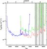 |
Fig. 1 Detection limits for the Lyα line, as a function of wavelength and redshift, for the three subsamples: Deep (green dashed line), Ultra-Deep red (red dotted line) and Ultra-Deep blue (blue line). The shaded regions indicate part of the spectra dominated by bright OH sky lines, where the rms of the background becomes too high to enable a secure line detection. |
The noise of VIMOS spectra varies as a function of wavelength, as a result of a combination of different effects. First, the combination of the efficiency of VIMOS optics and the CCD quantum efficiency depends on the wavelength of the incident light. Second, the OH airglow sky emission lines are in a several of bands which dominate the background for λ > 7500 Å, and are not easy to subtract from the combined object+sky spectra in low to medium resolution spectra. As a result, spectra are noisier at the wavelengths of the OH bands. An added uncertainty on the flux level is also sometimes present at the position of serendipitous Lyα emission because the background subtraction performed by the VIMOS data processing pipeline VIPGI (Scodeggio et al. 2005) is optimized using the knowledge of the position of the VVDS primary target. As the serendipitous target is offset from the main target, the low-order polynomial fit used to remove the background is made using some background points including the emission line, therefore artificially lowering the line flux. Third, the thin E2V detectors on VIMOS produce fringing which strongly affects the part of the spectra at λ > 8000 Å. As the VVDS has been using a low resolution R ~ 230 grism to maximize the number of objects in the survey, this produces a blend of the OH sky emission features, globally increasing the background noise at the position of the OH bands. As a result of these effects, the flux limit varies as a function of wavelength and therefore redshift. We determined the theoretical flux limit, separately for “Ultra-Deep blue”, “Ultra-Deep red” and Deep, by measuring the typical rms at different wavelengths in the 2-d spectra. Empirically, we decided to set the limit to 3σ in at least 5 contiguous pixels. The limits for the three subsamples are shown as a function of wavelength in Fig. 1. It can be noted that the background, even for each of the three subsets, is changing as a function of the wavelength and redshift. As a result of the bright OH skylines at λ > 7500 Å, a large part of the redshift range at z > 5.5 is in practice inaccessible. However, there are at least two very clean windows around z = 5.7 and z = 6.5, with a very low background corresponding to the absence of OH emission. The faintest flux limits can be observed in the range 4200 < λ < 7600 Å, reaching down to very faint flux levels of ~1.5 × 10⁻¹⁸ erg/cm2/s at 3σ. This combination of areal coverage, wavelength range, and depth is unprecedented.
2.2. Photometry
The VVDS 0216-04 field benefits from extensive deep photometry. The field was first observed with the CFH12K camera in BVRI bands (Le Fèvre et al. 2004; McCracken et al. 2003), in the U band (Radovich et al. 2004) and K band (Iovino et al. 2005). More recent and significantly deeper observations were obtained as part of the CFHT Legacy Survey in ugri and z′ (Goranova et al. 2009; Coupon et al. 2009), and as part of the WIRDS survey in J, H and K bands. The CFHTLS observations reach 5σ point source limiting magnitudes in i band of iAB ≃ 28 while the WIRDS observations reach a 3σ point source limit of KsAB ≃ 23.5 (Bielby et al., in preparation).
3. The Lyα sample
3.1. Serendipitous emission lines identification
The final sample consists of ~1200 2-d spectra observed with both red and blue grism (Ultra-Deep dataset), and ~8000 2-d spectra observed with the red grism. For each of the 92 quadrants observed, the reduction code (VIPGI, Scodeggio et al. 2005) produces a frame in which the ~100 2-d spectra are arranged one above the other, with the spectral direction along the x-axis. With the purpose of identifying serendipitous lines, we built a data processing procedure that automatically masked out all the continua and the bad features (bright residuals and OH skylines). The unmasked area is then used to search for emission lines, and to compute the effective area covered by each slit on the sky. An object falling serendipitously in a slit will produce a spectrum with a combination of continuum and emission lines. For faint objects with strong lines, the continuum is not detected, and we are left with emission lines with a line profile produced by the spectrograph. For point source objects, VIMOS produces a line profile along the slit (in the spatial direction) which is almost identical to the seeing profile (FWHM ~ 1′′ or about 5 pixels). This is the projected equivalent slit size resulting from the object size convolved with the seeing profile and the slit profile on the spectral dispersion direction for a maximum of about 5 pixels corresponding to the 1 arcsec slit width projection (or about 30 Å spectrally). The 2D line profiles produced are thus similar to point source images. For compact objects smaller than the atmospheric seeing disc, and if the seeing is smaller than the 1 arcsec slit width, the observed line profile in the spectral dimension will be dominated by the projected seeing profile. For extended objects the line profile becomes wider in the spatial direction leading to oval shaped emission lines. As these spectroscopic line images are similar to those of stars or galaxies on deep images, we blindly run SExtractor on the masked 2D spectra to automatically find all emission lines. This was followed by a visual inspection by two authors (PC and OLF) of all the objects detected by SExtractor, producing two independent candidate catalogs. A further inspection was conducted in order to find possible lines missed by SExtractor: we noted that lines too close to a bright continuum were not found by SExtractor, probably because of deblending problems. These two independent lists were then jointly examined by these two authors to decide if a candidate was to be kept, with more than 85% of the lists being unambiguously and independently selected by both authors. A fiducial catalog of bona-fide emission lines was then built from this comparison. A more careful determination of the incompleteness and contamination will be presented in the next sections. In particular, the completeness is assessed using simulations in Sect. 3.4, and an estimate of the contamination is given in Sect. 3.2.
Our final sample contains 133 serendipitous emission line emitters, 105 of which were found in the Ultra-Deep survey and 28 in the Deep. Most of these galaxies have no evident continuum in the spectra. We show a random selection of 8 serendipitous lines in Figs. 2 and 3. For each line, we show both the 2-d and 1-d spectra.
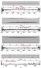 |
Fig. 2 Random selection of LAE candidates from the Ultra-Deep blue dataset, ordered by increasing redshift. For each of them we show the full 2-d (top) and 1-d (bottom) spectra. The position of Lyα is indicated by an arrow on both the 2-d and 1-d spectra, and by a label reporting the redshift on the 1-d spectrum. The observed wavelength scale at the bottom of the 1-d spectrum is transformed into the redshift of Lyα at each wavelength on the top. |
3.2. Lyα identification
Once the fiducial emission line catalog has been constructed, we have to unambiguously assign a rest-frame wavelength to any given emission line. If one emission line is identified in a contiguous spectrum covering 3600 to 9350 Å, there are several possibilities for the line identification assuming a star-forming galaxy spectrum: below 3727 Å the line is most probably Lyα, above 3727 Å the emission line can be Lyα, [OII]3727 Å, Hβ, [OIII]5007 Å (assuming [OIII]4959 Å is not detected, [OIII]5007/[OIII]4959 ≃ 3), or Hα. In the spectrum of normal star forming galaxies, [OII], Hβ and [OIII] are most often present. Therefore, as a first approach we assumed that the emission lines could be [OII] at 3727 Å, Hβ at 4861 Å, [OIII] at 5007 Å or Hα at 6563 Å, and we checked for other expected emission lines at different wavelengths in our spectral window. Using the typical line ratios for star-forming galaxies of average metallicity we estimate the flux of the other expected lines, and check whether they could be detected above our flux limit. However, the line flux ratios strongly depend on the galaxy metallicity. For example, typical ranges of line ratios are: [OIII]/[OII] = 0.1 ÷ 5, Hα/[OII] = 0.3 ÷ 5 and Hβ/Hα = 0.1 ÷ 0.8 (Lamareille et al. 2006; Maier et al. 2006; Tresse et al. 2007; Cowie & Barger 2008; Kewley & Ellison 2008). So, we decided to use the following line ratios, typical of galaxies with average metallicity: [OIII]/[OII] ~ 0.35, Hα/[OII] ~ 1 and Hβ/Hα ~ 0.35. Cases of extreme metallicity are discussed below.
Narrow-line type-II AGN with classical line ratios would be straightforward to identify given the broad wavelength range of our spectra. If we were to assign the single emissions lines to lines like CIV-1549, CIII-1909, or MgII-2800 we would expect to see other emission lines in our observed range either towards the UV (Lyα, CIV, CIII) or towards the red (MgII, [OII], [NeIII]). Broad line type-I AGN are also relatively easy to identify at our spectral resolution. We have not found any type-I or type-II AGN in our data, consistent with expected AGN counts in the area sampled (e.g. Bongiorno et al. 2007; Lamareille et al. 2009).
As the spectral window spans from 3600 Å to 9350 Å for the Ultra-Deep subsample and from 5500 Å to 9350 Å for the deep subsample, we analyze these samples separately.
-
Ultra-Deep: two single lines in the Ultra-Deep are at λ < 3727 Å, and then can identified as probably Lyα, while 103 are at λ > 3727 Å. Amongst the latter, 93 lines are at λ < 6920 Å. If they were [OII], we would have to have [OIII] and Hβ in our spectral window. We estimate, using the line ratios reported above, that 75 of these 93 lines should be accompanied by either detectable [OIII] or detectable Hβ or both but as they are not detected they are therefore most probably to be identified with Lyα. For the 10 emission lines at λ > 6920 Å, this argument cannot be used, because the possible [OIII] and Hα emission would lie outside our spectral window. Using similar arguments, we can infer that none of the Ultra-Deep lines are Hβ, [OIII] or Hα, because they would be always accompanied by at least one other line in our spectral window with a flux brighter than the flux limit.
-
Deep: the deep subsample contains 28 serendipitous lines. Again, all of them can be in principle interpreted as both Lyα or [OII]. Since for the Deep the spectral window is smaller than for the Ultra-Deep, the same argument as for the ultra-deep tells us that only 7 of these lines are not [OII]. For the other 21, either a possible [OIII] emission is outside the spectral range, or it would be too faint to be detected. However, we can conclude also that the bulk of them are not Hα, [OIII] or Hβ, because at least one other detectable line would be detected in our spectra.
From this first analysis, we can conclude that basically none of the serendipitous lines in the sample are Hα, Hβ or [OIII], that 84 among the 133 bona fide serendipitous lines are not [OII], and that most of the line identification uncertainty for the other 49 emission lines is between [OII] and Lyα. We note that these findings will not change too much if we had used much lower values for the metallicity. Assuming, for example, [OIII]/[OII] ~ 10, if the serendipitous line was assigned to [OII], we should always have detected [OIII] for all lines with λ < 6920.
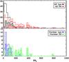 |
Fig. 4 top panel: for the full sample, the distribution of rest-frame EW if the lines are identified as Lyα (black histogram) or as [OII]3727 (red histogram). The filled histograms show objects without a detected continuum, for which the EW is a lower limit. lower panel: the same as the top panel, but for the 49 lines identified as ambiguous. The blue and green histograms represent respectively the rest-frame EW if the lines are identified as Lyα or as [OII]3727. |
We can perform a further check in order to evaluate the contribution of Lyα and [OII] emission to the observed population. In particular, we measured the observed equivalent width of the lines to produce the distribution of the rest-frame EW for each of the two cases, as presented in Fig. 4, for all the 217 lines as well as for the 49 ambiguous lines. While the distribution of the rest-frame EW for the lines if they are Lyα is mostly below 150 Å, we find that if the lines were assigned to [OII], ~70% of the distribution would be with EW[OII] > 100 Å. Among the 49 galaxies that cannot be unambiguously classified as either Lyα or [OII], 37 would have EW[OII] > 100 Å. We compare this distribution to the distribution of EW[OII] observed for galaxies with MB ≃ −18 in the VVDS-Deep (Vergani et al. 2008) in the same redshift range 0.86 < z < 1.5 and we note that 90% of the normal galaxy population has EW[OII] < 100 Å. At z ≃ 1, galaxies with EW[OII] > 100 Å have only rarely been observed in deep spectroscopy surveys, and none with EW > 150 Å (Hammer et al. 1997; Vergani et al. 2008). Since we expect to have just 5 lines with EW[OII] > 100 Å (10% of 49), we can conclude that for about 32 (37-5) the identification is very likely to be Lyα. So, at most we can identify the line as [OII] for 17 galaxies (49-32). We therefore conclude that about 10% of the single emission lines could be assigned to either [OII] or Lyα, while more 90% of them are most likely Lyα.
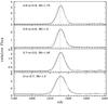 |
Fig. 5 Combined spectra for all serendipitous LAE in four redshift domains, centered on Lyα. The asymmetry of the line profile is clearly seen in each redshift range when comparing to a gaussian fit of the red wing of the line (long-dashed line). For each combined spectrum we report also the skewness calculated in the range 1201 < λ < 1231 Å. |
Another check on the line identification with Lyα is to look at the line profile. Lyα line profiles are most often asymmetric, with a truncation towards the blue because of absorption by the intergalactic medium, and an extended red wing because of complex velocity fields (Shapley et al. 2003; Ouchi et al. 2008). For individual objects, the line detection is not always of sufficient S/N to detect a line asymmetry, instead we produced the average normalized Lyα line profiles for LAE in different redshift ranges up to z ~ 6, as shown in Fig. 5 (the description of the combination technique and a more detailed analysis of the combined spectra are presented in Sect. 4.3). The asymmetry of the profile is clearly seen at all redshifts, even in the lower redshift bins. For each combined spectrum we measured also the skewness of the line in the range 1201 < λ < 1231 Å, which measures the degree of asymmetry of a given distribution. If the line profile would be perfectly described by a gaussian, that is by definition symmetric, the skewness would be zero. On the other hand, a positive value for the skewness indicates a distribution skewed towards red wavelengths. As Fig. 5 shows, in each redshift bin between 2 < z < 5.9 the skewness is positive and is increasing with redshift as expected from IGM absorption, reinforcing the primary identification with Lyα.
There are 6 galaxies with a single emission line in the atmospheric windows 8450 < λ < 8620 and 9000 < λ < 9300 clean of OH sky emission lines, and they observed equivalent widths 540 < EW < 1250 Å. If these lines were [OII]3727 or Hα, the rest EW would be 220 < EW < 510 or 400 < EW < 880 Å with a mean EW = 315 or 550 Å respectively, clearly outside the range of EW for [OII] or Hα emitting galaxies at z ~ 1. No sign of the broad component of an AGN which could produce high Hα EW was observed. We also computed the line profile of the 6 galaxies in this redshift range, reported in Fig. 6. The resulting profile is clearly asymmetric, as confirmed by the positive value for the skewness. As other single emission line candidates with strong observed EW are even more unlikely than [OII]3727 or Hα and should show other emission lines in our observed wavelength domain, we argue that the most likely possibility is that these emission lines are Lyα with 5.96 < z < 6.62, making them some of the most distant galaxies spectroscopically identified to date.
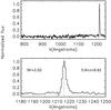 |
Fig. 6 Combined spectra for 5.9 < z < 6.62. The top panel shows the continuum bluewards of the Lyα line. The bottom one focuses on the line, showing the asymmetric profile. The value for the skewness of the line is also reported. |
In summary, among the 133 emission lines identified serendipitously in the 2D spectra, we conclude that 124 are most likely Lyα, while a low fraction of 14 (10%) can be either Lyα or [OII]. In the following, we assume that all galaxies with ambiguous line assignment are Lyα.
3.3. Final sample
We completed the LAE sample by adding the primary VVDS spectroscopic targets that unambiguously have Lyα in emission. We found 70 Lyα emitters among the ~1200 Ultra-Deep primary targets, all at redshift z < 3.5, and 14 among the ~8000 Deep targets. The Deep survey is actually limited to λ > 5500 Å, hence it could not detect Lyα at z < 3.5. All these galaxies have a high quality flag (larger than or equal to 2; Le Fèvre et al., in prep.) for the redshift, since they have other spectral features that allow one to unambiguously identify the redshift and therefore classify them as Lyα emitters. They show in fact OI at 1303 Å, CII at 1333 Å, SiIV at 1397 Å, CIV at 1549 Å, and sometimes CIII at 1909 Å. The final sample is therefore made of 217 LAE, including 133 serendipitous LAE, and 84 LAE from the primary VVDS targets. The sample is summarized in Table 1.
For each emission line, we carefully measured the position of the line (and thus the redshift), the total flux in the line and the continuum. The continuum, in units of Fλ, is measured as close as possible to the red wing of the Lyα line, by averaging the counts between 1230 and 1250 Å. From these fundamental quantities, the observed and rest-frame equivalent widths and the luminosities are derived: 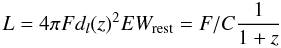 (1)where L and F are respectively the luminosity and the flux in the line, z is the redshift of the line, dl(z) is the luminosity distance at the redshift of the line, EWrest is the rest-frame Equivalent Width and C is the continuum around the line. Obviously, when the continuum is not detected, the derived equivalent widths are just a lower limit, and we used 1 sigma of the background as the continuum value.
Moreover, each luminosity can be converted to a SFR by using the well-known prescription to derive the SFR from Hα Luminosity by Kennicutt (1998) and the expected ratio between Lyα and Hα flux. In particular:  (2)with Hα flux corrected for internal extinction and valid for a Salpeter IMF. The conversion between Hα and Lyα luminosity was theoretically derived by Brocklehurst (1971) (assuming case B recombination):
 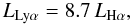 (3)and it does not account for dust and escape fraction corrections.
The final sample of Lyα emitters, divided into serendipitous objects and spectroscopic targets.
Combining the two gives:  (4)
(4)
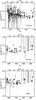 |
Fig. 7 For each sub-dataset, we show the flux versus redshift together with the flux limit as a function of the redshift and wavelength (solid lines). The flux limit is empirically measured on the 2-d spectra. Filled and open circles represent respectively serendipitous Lyα galaxies and targets with Lyα emission. |
In Fig. 7 we report the flux and the position (both wavelength and redshift if the lines are identified as Lyα) for the three surveys separately. It can be noted that the Ultra-Deep blue provides the largest sample with 164 emission lines galaxies (94 serendipitous lines and 70 targets from spectroscopy), while the Ultra-Deep red and the Deep contribute with respectively 24 and 42 emission lines galaxies. Note also that in a few instances we measure line fluxes that are weaker than the nominal flux limit at that wavelength: this is because the background, at each wavelength, is measured as the average of the backgrounds in the different quadrants and pointings. For some pointings, the background is lower than the average, and thus fainter lines can be detected.
3.4. Completeness simulations
As we saw in Fig. 1, the background of our spectra has a complicated structure as there are strong variations with wavelength. To perform a statistical analysis of the number density evolution of Lyα galaxies, it is important to carefully determine, for each wavelength (and thus for each redshift), what is our capability to recover a line with a given luminosity.
We performed a Monte Carlo simulation, building a catalog of 1000 fake lines for each dataset, for a total of 3000. Each line has a known flux, randomly extracted from a flat distribution between FLyα) = 1 × 10-18 and FLyα) = 1 × 10-16. The redshift is randomly extracted from a flat distribution between z = 2 and z = 4.7 (for blue spectra) and between z = 3.7 and z = 6.7 (for red spectra). The fake lines are then added at the wavelength corresponding to the known redshift, in a randomly extracted slit. Since emission lines in our sample are not or barely resolved either in the spatial or in the spectral directions (see next sections), we chose to use simple gaussian profiles with FWHM of 1′′ × 30 Å.
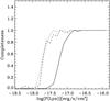 |
Fig. 8 Completeness in line identification from Monte Carlo simulation as a function of the flux, for the three subsamples: Deep (solid line), Ultra-Deep red (dotted line) and Ultra-Deep blue (dashed line). |
We attempted to recover these simulated lines, without a-priori knowledge of redshifts and fluxes, by applying the same procedure used on the real 2-d spectra, described in Sect. 3.1. The results are reported in Fig. 8 presenting the completeness as a function of the line luminosity and of the redshift, for the three subsamples. We can see that Ultra-Deep blue & red and Deep are 50% complete respectively at FLyα ~ 2 × 10-18 and ~8 × 10-18.
3.5. Slit flux loss
Since the slits used have sizes comparable to the seeing of the images, part of the line flux cannot be recovered and will be always lost. The flux loss depends on the offset between the galaxy and the slit center positions, on the size of the galaxy with respect to the slit width and on the atmospheric seeing. For an object perfectly centered in the slit, the flux loss will be minimal, but not zero. If the position of the object in the slit is known, as in the case of the objects with an optical counterpart, it is relatively easy to compute the flux loss. However, a significant number of galaxies in our sample do not have an optical counterpart within ±0.5′′ from the expected position of the object along the slit and within ±2′′ off axis in the direction perpendicular to the slit (see Sect. 4.2).
As we do not know for these galaxies their positions inside the slits, we cannot compute for each object the actual flux lost. This problem is common to all surveys of serendipitous Lyα emitters (e.g. Rauch et al. 2008; Lemaux et al. 2009), and is usually solved with a statistical approach for the objects with no detected counterpart. In this section, we derive the slit flux loss as a function of the position of the object in the slit, so that we can correct the line flux for those objects with an optical counterpart, and then we estimate a statistical correction for the objects without any optical counterpart.
We start from the consideration that the bulk of our Lyα galaxies are unresolved in the spatial direction (see Sect. 4.2), having sizes comparable with the seeing of the observations. The FWHM distribution in the spatial direction of the lines in our sample ranges from 0.5 to 1.2 arcsec, with 90% of them having FWHM = 0.7 ÷ 1.2 arcsec (see Fig. 11). This implies that we can model them as gaussians, with fixed FWHM. We built a simulation in which an emission line object with a given FWHM is placed in a 1 arcsec slit at different positions with respect to the center of the slit until it is completely outside of the slit width. The small inset in Fig. 9 shows the fraction of recovered flux as a function of the offset between the objects and the slit, for three seeing conditions FWHM = 0.7, 0.9 and 1.2 arcsec (corresponding to σ ~ 0.3, 0.38 and 0.5 arcsec). If the galaxy was perfectly centered in the slit, only ~70, 80 and 90% of the flux would be recovered, respectively for the 1.2, 0.9 and 0.7 arcsec FWHM lines; on the other hand, if the galaxy would be placed at 2σ = 0.8 arcsec outside the slit, only 20% of the light would be retrieved.
Thus, we can estimate that the slit flux loss for the 84 primary spectroscopic targets, that are perfectly centered in the slits, is around 15%, with a typical range between 10% and 30% depending on the seeing. For the serendipitous object with an optical counterpart, whose offset with respect to the center of the slit is known, we estimated the flux loss assuming they are compact under the average seeing conditions of a pointing. We show their distribution of the recovered flux in Fig. 9.
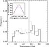 |
Fig. 9 Histogram of the percentage of recovered flux, for a set of a 3000 simulated lines randomly offset with respect to the center of the slit (solid line) and for the serendipitous lines (dotted line). The vertical lines show the median for the two distributions, around 55% of the recovered flux. The small inset shows the recovered flux as a function of the offsets for the simulated lines, for the 0.7, 0.9 and 1.2 arcsec FWHM lines (respectively in red, black and blue). |
In order to check if the percentage of recovered flux that we find for the serendipitous sample is reasonable we use a Monte Carlo simulation. In particular, we generate 3000 2-dimensional gaussian profiles with FWHM randomly extracted between 0.7 and 1 arcsec, applying an offset between the position of the peak and the center of the slit randomly extracted between ±1 arcsec. The distribution of the recovered flux for the 3000 lines is shown in Fig. 9. We note that the choice of ±1′′ as maximum offset introduces an artificial cut-off at ~10% of the recovered flux. This choice however is justified by the fact that an hypothetical object placed offslit by more than ±1′′ should have a true Lyα flux > 10 × stronger than the one measured in the slit spectroscopy, hence its optical counterpart should be visible in photometry. There is an overall agreement from the result of this simulation and the flux loss estimated for the serendipitous lines with optical counterpart. For ~40% of the cases, the recovered flux is higher than 70%. The median of both histograms is ≃55%: we will use this value to correct the measured fluxes for the serendipitous lines with no optical detection in our sample.
4. Sample properties
4.1. Redshift distribution
In Fig. 10 we show the redshift distribution for our sample. The distribution extends from z = 2 to z = 6.7, with a median ⟨ z ⟩ = 3. We have 5 detections at z ~ 6.5 and 9 at z ~ 5.7. The main VVDS targets with Lyα come mainly from the Ultra-Deep survey, and interestingly, they show a different redshift distribution: even though the peak for the two subsamples is around z = 2.2 ÷ 2.5, the serendipitous sources show a broader tail at z > 4, while 85% of the targets have z < 4. A simple Kolmogorov-Smirnov test rules out with more than 99% confidence that the two distribution are statistically equivalent. This reflects the different selection for the two subsamples: magnitude selected for the former, flux selected for the latter.
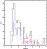 |
Fig. 10 Redshift distribution for the whole sample (black line), as well as for the different subsamples: solid lines show serendipitous lines, while dotted ones indicate primary spectroscopic targets; blue and red lines show the Ultra-Deep and deep subsamples, respectively. |
4.2. Optical counterparts and size distribution
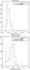 |
Fig. 11 Full width half maximum (FWHM) distribution as measured from the CFHTLS images (top panel) and from the Lyα 2-d spectra (bottom panel). Targets are shown with a solid line, serendipitous objects with and without photometric counterparts are shown with a dotted and dashed line, respectively. The CFHTLS image used was built by stacking the 25% best-seeing exposures, and has a final PSF FWHM of about 0.5′′. In the top panel, we just show serendipitous objects with a photometric counterpart. |
We searched the deep CFHTLS ugriz images, including the combined ugriz stack, for optical counterparts of the 133 serendipitous LAE. In order to account for possible positional uncertainties, we required the counterpart to be within ±0.5′′ from the position of the spectrum along the slit. Moreover, since even bright off-slit objects can show a detectable spectrum (see Sect. 3.5), we search for counterparts within ±2′′ of axis. We found faint counterparts for 53 (50%) and 13 (46%) LAE respectively in the ultradeep and in the deep sample, with magnitudes iAB ranging from 23.5 to 27.5. These counterparts are always ±1′′ off axis at the most. For the remaining 67 objects we did not find an optical counterpart down to a magnitude AB ~ 28.
In Fig. 11 we compare the Full Width at Half Maximum (FWHM) for the serendipitous Lyα emitters and the spectroscopic targets, as measured on the deep CFHTLS images and directly on the 2-d spectra of the Lyα line.
In particular, we used CFHTLS-D1 (VVDS-02h field) D-25 stack in the z-band, that was built stacking the 25% best seeing images together resulting in a PSF FWHM of about 0.5 arcsec (see Table 26 of Goranova et al. 2009). Thanks to the better angular resolution, these images are very useful to check whether or not our galaxies are resolved in the spatial direction. On the other hand, we are also interested in measuring the size for our sample also on the 2-d spectra to check the assumption we made in Sect. 3.5 where we estimated the slit flux loss.
The FWHM of the serendipitous and main VVDS magnitude selected populations with optical counterparts measured in the D-25 stack are compared in the top panel of Fig. 11. The distribution for both populations peaks at around 0.5 arcsec with a gaussian distribution width. This is expected from the measurement errors on these faint objects if they are unresolved under the seeing of the D-25 stack. The width of the Lyα line measured on the 2-d spectra (bottom panel of Fig. 11) indicates that the Lyα line is emitted from a compact region, as the size distribution is comparable to the seeing distribution of the spectroscopic observations. This therefore indicates that most of the LAE are compact both in the continuum and for line emission.
From these measurements it is clear that the faint LAE population is compact in size. Interestingly, there is a clear lack of large objects (FWHM > 1−1.5 arcsec) in our sample. Faint LAE clearly have different sizes than the large Lyα blobs identified in the bright LAE population (Steidel et al. 2000; Matsuda et al. 2004; Ouchi et al. 2008). The weak continuum and Lyα sizes are in agreement with Venemans et al. (2005), Taniguchi et al. (2009), and the HST-based study of Bond et al. (2010). Our results support a picture where Lyα emission from faint LAE is compact and originates from the same area as the UV continuum as found by Bond et al. (2010), and we do not confirm the trend reported by Nilsson et al. (2009) of more extended sizes in the narrow band Lyα images than in the broad-band images. While extended Lyα emission like observed in Lyα blobs and Lyα halos is expected if Lyα is produced from resonant scattering on diffuse gas surrounding the galaxy, our data may indicate that the gas reservoir of faint LAEs is rather compact or that, if extended, it is only scattering a small fraction of the Lyα photons. We will explore the evolution with redshift of these properties in a forthcoming paper.
We show the size distribution measured directly on the 2-d spectra in the bottom panel of Fig. 11: due to the poorer seeing of these observations with respect to the CFHTLS ones, this distribution is peaked at 0.9 arcsec. Hence, this justifies our choice to simulate lines as gaussians with an average FWHM of 0.9 arcsec to estimate the slit flux loss in Sect. 3.5.
4.3. Spectral properties of the LAE
We produced combined spectra for all the Lyα in our sample, including primary VVDS targets as well as sources identified serendipitously. In order to preserve line shapes and to avoid averaging out faint features, we used accurate redshift measurements from a half-gaussian fit to the red wing of the Lyα lines which was used to determine the central wavelength of Lyα and therefore the redshift. Each spectrum was then shifted to rest-frame, normalized using the continuum flux in 1400−1800 Å up to z = 4.6, 1400−1600 Å for 4.6 ≤ z ≤ 5.9, and the Lyα line itself for 5.9 < z ≤ 6.7, then averaged using a sigma-clipping algorithm. The results in several redshift ranges are shown in Figs. 12 and 13, for serendipitous and target objects, respectively. A number of spectral features can be readily identified at all redshifts, including of course Lyα, but also prominent CIV in absorption as well as HeII in emission well detected in the two lowest redshift bins.
Bluer than Lyα we can see that the continuum is more absorbed as redshift increases, with a ratio (f [1250−1350 Å] / f [1100−1180 Å] ) for serendipitous LAE of 1.34, 1.47, 2.0, 9.3 for redshifts z ~ 2.3, 3, 4, 5.3 respectively, and for target LAE a ratio of 1.41 and 1.51 for redshifts z ~ 2.3, 3 respectively. For our highest redshift objects 5.9 < z < 6.7, uncertainties on the continuum blueward of Lyα only enables us to state that this ratio is higher than 5. These measurements are comparable to the expected average extinction by the intergalactic medium, as Madau et al. (1995) predict ratios of 1.3, 1.5, 2.5 and 8.2 for z ~ 2.3, 3, 4, 5.3, respectively. This strengthens our identification of these emission line objects as LAE.
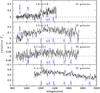 |
Fig. 12 Combined spectra of the serendipitous Lyα emitters, in several redshift ranges from z = 2 to z = 5.9. The displayed range of flux was selected to show faint continuum features, while the peak of the Lyα line is largely off-scale. Blue dotted lines indicate different spectral features depending on the redshift range: Ly-break at 912 Å, Lyβ at 1026 Å, OI at 1303 Å, CII at 1333 Å, SiIV at 1397 Å, CIV at 1549 Å, HeII at 1640 Å and CIII at 1909 Å. The horizontal dashed lines indicate the level of zero flux. |
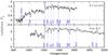 |
Fig. 13 Combined spectra of the target Lyα emitters in the redshift ranges 2 ≤ z ≤ 2.7 and 2.7 ≤ z ≤ 3.5. The displayed range of flux was select to show faint continuum features, while the peak of the Lyα line is largely off-scale. The horizontal dashed lines indicate the level of zero flux. |
Lyβ − 1026 Å is readily observed, and the Lyman-break at 912 Å is well detected for redshifts z > 2.9 placing this feature in our observed wavelength range, as expected.
To check for a difference between the targeted magnitude limited sample and the serendipitous LAE, we produced the combined spectra for all target LAE in the redshift domains 2 ≤ z ≤ 2.7 and 2.7 < z ≤ 3.5 as shown in Fig. 13, while above z = 3.5 the serendipitous LAE dominate and their combined spectra are almost identical to the spectra shown in Fig. 12. Many spectral features are clearly detected in absorption: Lyβ −1026 Å, OI−1303 Å, SiIV−1397 Å. Besides Lyα, CIV−1549 Å, HeII−1640 Å and CIII−1909 Å are all detected in emission.
The Lyα rest-EW increases from 38 ± 1 Å at z ≃ 2.3 to 370 ± 150 at z ≃ 6.3. This trend is probably the result of two effects: a general trend of increasing star formation at higher redshifts and a difference between the observed galaxy populations, with less (more) luminous galaxies observed at lower (higher) redshifts. The mean EW of HeII−1640 for the full sample is EW = 1.4 ± 0.2 Å, 2.0 ± 0.1 Å and 4.0 ± 2.0 Å at z ≃ 2.3, z ≃ 3.1, and z ≃ 4 respectively, indicating the presence of a young stellar population a few 107 years old (Schaerer 2002). Considering only the serendipitous Lyα, the EW(HeII) rises from 3.9 ± 0.4 at z ≃ 2.3 to 14.5 ± 1.5 at z ≃ 3.1. This clearly indicates that a younger stellar population is present at the higher redshift. The difference of EW between the full Lyα sample and the serendipitous Lyα at z ≃ 3.1 is significant, 4.0 ± 2.0 versus 14.5 ± 1.5, possibly again a consequence of the different populations observed, Lyα in the serendipitous sample corresponding to fainter objects with stronger star formation or less extinction of the Lyα emitted photons. This difference at the same redshift could therefore indicate that continuum-faint Lyα contain younger stellar populations than continuum-bright Lyα. This will be the subject of future studies.
The Lyα line in the combined spectra has an asymmetric profile with the blue wing truncated and an extended red wing, as shown in Fig. 5. This is expected as gas outflow and intergalactic absorption impose a sharp blue cutoff and a broad red wing. This Lyα shape and the clear detection of other expected emission and absorption features in the combined spectra provides further supporting evidence that the bulk of the lines in our sample are Lyα rather than [OII].
4.4. Properties of the 6 galaxies with 5.96 ≤ z ≤ 6.62
The combined spectrum of the 6 galaxies identified with 5.96 < z < 6.62 is shown in Fig. 6. The continuum below Lyα is barely detected in this redshift range, consistent with a strong absorption by the intergalactic medium, while we detect a continuum at the 2σ level above 1215 Å. The line profile shown in Fig. 6 is also asymmetric in this redshift range, reinforcing the identification of the emission lines with Lyα.
The distribution of rest EW(Lyα) is in the range 70 < EW < 500, with a mean EW = 310 Å and a dispersion of 150 Å. Malhotra & Rhoads (2002) suggested that EW > 300 Å may indicate a top-heavy IMF. However, our measurements are just at this limit, and moreover very uncertain, so we cannot draw any conclusions on this issue. Moreover, using Eq. (4) to convert luminosities to SFR for these 6 galaxies we obtain SFRs in the range 4 < SFR < 22 M⊙ yr-1, values that are not so extreme as to require a top-heavy IMF.
None of these galaxies are photometrically detected, neither in the single bands reaching as faint as iAB = 28 (1σ), nor in the combined ugirz image, reaching an equivalent magnitude of AB ≃ 29.
4.5. Photometric properties
In Figs. 14 and 15 we show the ugr and gri diagrams for all galaxies in our sample (serendipitous and targets) at 2.6 < z < 4.2. In fact, young star forming galaxies usually display very red colors around the 912 Å Lyman limit: the flux below 912 Å is virtually zero thanks to strong IGM absorption, while the star formation activity produces strong emission beyond Lyα line, producing a very pronounced and high S/N feature. This peculiarity used extensively used to search for high redshift (z > 2) galaxies (e.g. Steidel et al. 1999; Giavalisco 2002; Bouwens et al. 2007, 2009, 2010). We determined the part of the color − color plots in which high-z “dropouts” are expected to be by convolving synthetic spectral energy distributions for star-forming galaxies with the SDSS photometric system filters.
In Fig. 14, about 80% of the galaxies with 2.6 < z < 3.6 fall in the expected u-band dropout region. Similarly, in Fig. 15, about 50% of the galaxies at 3.6 < z < 4.2 fall in the expected g-band dropout region. The fact that a significant fraction of objects with secure spectroscopic redshifts falls out of the predicted color selection boxes was already noted by Le Fèvre et al. (2005), also for LAE as Gronwall et al. (2007) find a significant fraction of their sample outside of a UVR LBG box, and is mainly the result of the photometric measurement process (Le Fèvre et al., in prep.).
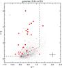 |
Fig. 14 UGR color–color plot for galaxies in our sample between 2.6 < z < 3.6. Filled and open circles represent respectively targets and serendipitous objects with optical counterpart. Black points show galaxies at all redshifts. The dashed box indicates the drop-out region in which galaxies at such redshifts are expected to lie. The cross in the bottom right part of the diagram shows the typical error bars. |
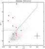 |
Fig. 15 GRI color–color plot for galaxies in our sample between 3.6 < z < 4.2. Filled and open circles represent respectively targets and serendipitous objects with optical counterparts. Black points show galaxies at all redshifts. The dashed box indicates the drop-out region in which galaxies at such redshifts are expected to lie. The cross in the bottom right part of the diagram shows the typical error bars. |
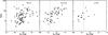 |
Fig. 16 Equivalent Width of the Lyα line as a function of the absolute magnitude at 1600 Å, for the objects with photometric counterpart, in three different redshift bins. Objects with detected continuum are shown as filled dots. Objects without a detected continuum, for which the equivalent width is only a lower limit, are shown as upperward arrows. The dotted line shows MUV = −21.5: objects brighter than this limit show a deficit of large equivalent widths (EW0 > 20). |
In Fig. 16 we plot, for the objects with a photometric counterpart (primary targets and serendipitous), the equivalent width of the Lyα lines as a function of the absolute magnitude in the UV at λrest = 1600 Å, for three different redshift bins. Shimasaku et al. (2006), Ando et al. (2006) and Ouchi et al. (2008) suggested that objects with MUV < −21.5 show typically low equivalent width (EW < 20), while objects with MUV > −21.5 span a wide range of EW (50 < EW < 150). Our data are consistent with these findings, even though some of our galaxies with MUV < −21.5 have just a lower limit to the EW. We note also that many of the serendipitous galaxies do not appear in this figure, as they have no photometric counterparts.
In Fig. 17 we compare the Lyα Luminosity, the Lyα Equivalent Width and the SFR inferred from the Lyα Luminosity for galaxies in our sample with others in literature. The aim of this figure is to show the different selection criteria for the various samples of Lyα emitters. Narrow band surveys typically select objects with EW0 > 20 and do not reach Lyα emitters less luminous than LLyα = 1041.5, while our sample has no limits on the equivalent width and goes 0.5−1 dex deeper in luminosity. Overall, all the samples seem to follow a broad relation between Lyα luminosity and Lyα equivalent width. Moreover, it is clear that the typical object in our sample has a SFR ~ 1 M⊙ yr-1, with many having even smaller rates, while other samples have typically SFR > 1 M⊙ yr-1, as expected from our deeper flux limit.
5. Luminosity functions
5.1. Formalism
We aim to combine the serendipitous and target Lyα emitters in the U-DEEP and DEEP surveys to produce luminosity functions at different redshifts. Since the targets and serendipitous objects have very different selection criteria, for the luminosity function calculation we treated them independently. So, each galaxy from the target sample has a weight calculated with respect to the photometric selection, and each galaxy from the serendipitous sample has a weight calculated with respect to the spectroscopic selection.
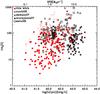 |
Fig. 17 Luminosity versus equivalent width for the galaxies in our sample (red points); filled and open circles indicate respectively galaxies with and without a detected continuum. For the latter, the measure of the EW is a lower limit. Black diamonds, triangles, crosses and squares show respectively the samples of Ouchi et al. (2008), Dawson et al. (2007), Murayama et al. (2007) and Saito et al. (2008). |
Each of the two samples, however, are a combination of subsamples having different magnitude or Lyα flux limits and covering different areas: serendipitous LAE were identified because their line flux exceeds the spectroscopic flux limit; those coming from the Ultra-Deep have a flux limit ~1.5 × 10⁻¹⁸ erg/cm2/, while those coming from the Deep survey have a flux limit of ~5 × 10-18 erg/cm2/s. The VVDS primary spectroscopic targets are selected according to their magnitude in the I-band; those coming from the Ultra-Deep are selected to have mI < 24.75, and those coming from the Deep to have mI < 24.
To combine together subsamples reaching different flux (or magnitude) limits in different areas, we used the extended version of the 1/Vmax formalism developed by Avni & Bahcall (1980). For each object we computed two effective volumes Vmax(j), one for the ultradeep limit and the other for the deep one (if the object is a target, the limit is the magnitude limit, if the object is a serendipitous one, the limit is the Lyα flux limit). So, for an object with redshift z assigned to the redshift bin z1 < z < z2: 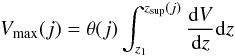 (5)where zsup is the minimum between z2 and the redshift at which the object could were observed within the limits of the jth selection, θ is the solid angle covered by the jth survey, and dV/dz is the comoving volume element. For each object, Vmax is defined as:
 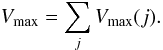 (6)This basically means that the brightest objects which are visible in both the ultradeep and deep surveys are weighted according to the effective volume accessible to them in both surveys, while the faintest one which are visible on in the ultradeep survey are weighted just with respect to the latter. The target sampling rate and the success rate were taken into account in computing the volumes for the targets. They are ~0.1 and ~0.3 for Ultradeep and Deep surveys, respectively.
The Lyα luminosities were here corrected for the flux slit loss, as explained in Sect. 3.5: for the targets, the expected slit loss is 15%, and for the serendipitous sample is ~45%. We verified that the choice of an average value for such correction do not affect our main results: in particular, the Schechter best-fit values presented in Sect. 5.2 do not change, within the errors, if the slit flux loss correction are randomly extracted for each object from the distribution shown in Fig. 9. Finally, we combined the two Vmax for them using Eq. (6). Moreover, a completeness correction was applied to each object according to its flux and redshift, both for targets and for serendipitous emitters.
Once we have Vmax for both the targets and serendipitous objects, we compute the galaxy number density for each Δlog (L) and Δz bin as follows: 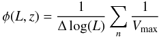 (7)where n is the number of objects in that bin.
5.2. Evolution of the luminosity functions
We estimated the luminosity functions for 3 redshift bins: z = 1.95−3., z = 3.−4.55, z = 4.55−6.6 in order to keep enough galaxies per redshift bin for a reliable estimate of the LF. The results are shown in Fig. 18.
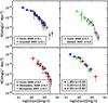 |
Fig. 18 LAE luminosity function in different redshift bins. No IGM absorption correction was applied here. Upper left, upper right and bottom left panels indicate 2 < z < 3.2, 3.2 < z < 4.55 and 4.55 < z < 6.6 respectively. The error bars reflect the Poissonian errors. Black points show literature data, spanning from z = 3 to z = 5.7: diamonds, triangles and squares represent Ouchi et al. (2008) at respectively z = 3.1, z = 3.7 and z = 5.7; asterisks, plus signs, crosses and circles indicate respectively Shimasaku et al. (2006) at z = 5.7, Murayama et al. (2007) at z = 5.7, Gronwall et al. (2007) at z = 3.1 and Dawson et al. (2007) at z = 4.5. We group together our measurements in the different redshift bins in the bottom right panel, to show that within the error bars, the Lyα LF does not evolve from z = 2.5 to z = 6. |
When comparing our data in these different redshift intervals, we can see that the observed apparent luminosity function (i.e. the non-IGM corrected LF) does not evolve in the redshift range z ≃ 2.5 to z ≃ 6 within our error bars. Although our data cover a slightly wider redshift interval they are in agreement with the literature data, within errors. This is quantified below.
The unprecedented depth of our survey enables us to extend the luminosity function at z = 2−3. down to log (LLyα) = 41.3, about one order of magnitude deeper than literature data at similar redshifts. This allows us to strongly constrain the slope of the luminosity function at z ~ 2.5. This parameter is extremely important, because a small change of this slope can produce a large change in the luminosity density.
We assumed here that the luminosity function of Lyα emitters is well represented by a Schechter law (Schechter 1976):  (8)We obtained the best-fit functions for the 3 redshift bins using this Schechter function. As a first try, we fitted the luminosity functions in the 3 redshift intervals allowing all the 3 parameters describing the Schechter function to vary. However, by doing this, the typical luminosity L∗ in the first two bins and the slope α in the high redshift bin are poorly constrained. Indeed, in the first two bins we do not have Lyα galaxies brighter than 1043 erg/cm2/s, and in the last one we do not observe emission lines fainter than 1042 erg/cm2/s. For this reason we decided to use other datapoints in the literature to constrain L∗ in the first two bins. In particular, we averaged the L∗ values obtained by Ouchi et al. (2008) and Gronwall et al. (2007) at z = 3.1, obtaining log (L∗) = 42.7. So, in our fit procedure we fixed log (LLy − α) = 42.7 in the first two bins. We verified that this approach is equivalent to including Ouchi et al. (2008) and Gronwall et al. (2007) datapoints with log (LLyα) ≳ 43 to ours and performing the fit. Moreover, we constrained α in the last bin to the average of the value in the first two bins. The best-fit parameters are reported in Table 2.
Schechter function parameters.
Importantly, we note that the luminosity functions reported above are not corrected for absorption by the intergalactic medium. The Lyα flux from high-z sources is generally absorbed by neutral hydrogen present in the IGM, that absorbs the blue wing of the Lyα line, producing an asymmetric line profile (Hu et al. 2004; Shimasaku et al. 2006). We therefore measure IGM absorbed Lyα fluxes, and not intrinsic Lyα fluxes. Moreover, the amount of absorption is not the same at different redshifts: at high z the amount of intervening intergalactic medium is larger. As a consequence, if the observed i.e. apparent luminosity functions do not evolve from z ~ 2.5 to z ~ 6, the intrinsic one positively evolves. The IGM optical depths were estimated in various studies (i.e. Madau 1995; Fan et al. 2006; and Meiksin 2006): all the authors agree that the amount of absorption increases from ~15% at z ~ 3 to ~50% at z ~ 6 (at this redshift, basically all the blue side of the line is absorbed). Using the standard radiative transfer prescription from Fan et al. (2006) for the IGM optical depths, we can obtain the intrinsic luminosities Lint from the observed Lobs. At z ~ 2.5, 4.2 and 6 the ratio Lobs/Lint is respectively 0.91, 0.73 and 0.52.
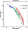 |
Fig. 19 We report here our estimates of the intrinsic luminosity functions, corrected for the IGM absorption (shaded regions). Blue, green and red indicate respectively 1.95 < z < 3, 3 < z < 4.55 and 4.55 < z < 6.6 ranges. Solid lines show our best fits to the data. |
In Fig. 19 we show instead the intrinsic luminosity functions, corrected for the IGM absorption according to the prescription of Fan et al. (2006), together with our Schechter fits to the data.
The first major result from this analysis is that there does not seem to be a strong evolution of the apparent luminosity function between z ~ 6 and z ~ 2.5, within our error bars. In fact, looking at Fig. 18 we see that within our 1σ errors, the luminosity functions in the different redshift bins overlap; moreover, looking at the Schechter best fit parameters in Table 2, we can see again that within 1σ the Schechter parameters do not evolve. On the other hand, by looking at the intrinsic luminosity functions in Fig. 19, we do see an evolution between z ~ 6 and z ~ 4, while no sizeable evolution is observed between z ~ 4 and z ~ 2. The observed evolution can be parametrized with the evolution in L∗, that is at z ~ 6 about 1.8 times higher than in the first bin. However, its significance level is only 1.5σ.
The second interesting result comes from our ability to constrain the faint end of the luminosity function. We find slopes  at z ~ 2.5 and
  at and z ~ 4. Our data formally exclude a flat slope α ~ −1 at 5 and 6.5σ, at these two redshifts. Our slope values are significantly better constrained than the best value of 1.36 and the marginalized value of
  found at z ~ 3.1 by Gronwall et al. (2007), a consequence of the 10 times fainter flux limit of our sample. Note that other authors, who again do not have deep enough data, do not try to fit α, but they rather fix it to some plausible value (−1, −1.5 and −2 for Ouchi et al. 2008; −1.6 for Dawson et al. 2007; −1.2 and −1.6 for Lemaux et al. 2009). Our analysis therefore establishes the first reliable estimate of the faint end slope of the luminosity function of Lyα galaxies at z < 5.
It is also important to state that the possible “non-Lyα” emitters in our sample, described in Sect. 3.2, do not strongly affect these results. First of all, the luminosity distribution of the “ambiguous” lines (the 49 lines that cannot be unambiguously identified as Lyα based on the line ratios) is similar to that of the global sample, and thus it is not expected to affect the slope determination. However, it is possible that in the 4.55 < z < 6.6 redshift bin the contamination is higher than in the others. In fact, for all the lines at λ > 6920 (corresponding to z(Lyα) ≳ 4.7), we cannot check for other lines in the spectra, if the line is identified as [OII] (see Sect. 3.2). However, we showed that the contamination is not expected to be higher than 10%, based on the EW distribution. Thus, assuming that all the 17 lines that can be identified as [OII] are at z > 4.7 would decrease the luminosity function in the last bin of a factor of 50% at the most. This would imply a weaker evolution of the luminosity function from z = 6 to z = 4.
5.3. Evolution of the star formation rate density
With these new constraints on the evolution of the Lyα luminosity function at these redshifts, it is interesting to estimate the contribution of the Lyα emitters to the global SFRD of the Universe. This is not trivial, as Lyα emission produced not only by star formation activity, but also by other processes like cooling radiation, AGN activity or shock winds. Moreover, Lyα emission is attenuated by IGM and dust.
We compute here the SFRDs using only the intrinsic Lyα luminosity functions. In order to estimate the contribution of the galaxies in our sample, we integrated the luminosity function from LLyα = 0.04 × L ∗ to log (LLyα) = 44 (roughly the interval covered by our data). We then converted these Lyα luminosity densities in SFRDs by using Eq. (4).
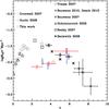 |
Fig. 20 Evolution of the SFRD as a function of the redshift, inferred integrating the intrinsic Lyα luminosity functions down to 0.04 × L ∗ . Red open circles are our data, while blue and green open circles represent other Lyα SFRD respectively by Ouchi et al. (2008) and Gronwall et al. (2007). Open triangles, open squares, open lozenges, stars and crosses are UV estimates respectively by Schiminovich et al. (2005), Reddy et al. (2008), Bouwens et al. (2007), Beckwith et al. (2006), Tresse et al. (2007) and Bouwens et al. (2010). |
The derived SFRs are shown in Fig. 20, together with the most recent estimates of the SFRD at redshift between z = 0 and z = 6. Ouchi et al. (2008) and Gronwall et al. (2007) use a sample of narrow band selected Lyα emitters, while the other estimates are based on the UV galaxy luminosity function.
We can see that our measurements show a slight evolution of the Lyα SFRD between z ~ 2.5 and z ~ 4, and a much more significant evolution from z ~ 4 and z ~ 6. Our values are compatible within the errors to those obtained by Ouchi et al. (2008).
When comparing our estimates of the Lyα SFRD with the UV-derived ones, we see that the total contribution of Lyα galaxies to the global SFRD at z ~ 2−6 is important, increasing from ~20% at z ~ 2.5 to ~100% at z ~ 6. This implies that the Lyα emission is a good tracer of the star formation, this statistically implies that, while at redshift z ~ 2 only a small fraction of the galaxies contributing to the star formation history of the universe also show a Lyα emission, all the galaxies at z ~ 6 do show Lyα in emission. In other words, the so called escape fraction, that is the fraction of Lyα emission produced by the star formation that actually escapes the star formation regions changes a lot with the cosmic epoch, from 20% at z = 2.5, reaching up to 100% at z ~ 6. This seems to indicate that the mechanism which is absorbing the Lyα photons in most of the galaxies at z = 2 is not effective at z ~ 6, as is expected in a very low dust medium. However, dust estimates at z ≃ 5−6 show that the dust content should be sufficient to produce significant Lyα photons absorption (e.g. Bouwens et al. 2009).
Alternatively, it is possible that the UV luminosity function based on Lyman break galaxies searches is based on more and more incomplete counts at increasingly high redshifts, and that the current UV-derived SFRD are underestimates (e.g. Le Fèvre et al. 2005; Paltani et al. 2007). Current estimates of the luminosity density at z ≃ 5−6 agree within a factor 2−3 or so (Bouwens et al. 2007, 2009), and will require a new generation of surveys to be improved.
6. Summary
In this paper we have reported the discovery of 217 faint LAE in the range 2 ≤ z ≤ 6.62 from targeted and serendipitous very deep observations using the VIMOS multi-slit spectrograph on the VLT. Adding together the areas covered by each slitlet combined to the wide wavelength coverage 5500−9350 Å of the Deep survey and 3600−9350 Å for the UltraDeep, we surveyed effective sky areas of 22.2 arcmin2 and 3.3 arcmin2 respectively. This produces a survey volume of ~2.5 × 10⁵ Mpc3, observed to an unprecedented depth of F ~ 1.5 × 10⁻¹⁸ erg/s/cm2. This volume is about one order of magnitude larger than all other spectroscopic surveys produced up to now at comparable fluxes: van Breukelen et al. (2005) sampled 104 Mpc3 down to 1.4 × 10⁻¹⁷ erg/cm2/s; Martin et al. (2008) sampled 4.5 × 10⁴ Mpc3 down to similar fluxes in a narrow redshift range. Narrow band imaging surveys sampled greater volumes than ours, but to shallower flux limits: Ouchi et al. (2008) covered a volume of ~106 Mpc3, down to fluxes ~2 × 10-17 erg/cm2/s. Serendipitous surveys have been found lower number of objects (Sawicki et al. 2008), even if reaching somewhat deeper (Malhotra et al. 2005; Rauch et al. 2008). We are therefore sampling deeper into the LAE luminosity function as we discussed in Sect. 5.2.
From an observational point of view, we demonstrate the efficiency of blind LAE searches with efficient multi-slit spectrographs. The success of our approach is the result of combining a broad wavelength coverage to a large effective sky area, with long integration times, made possible by the high multiplex of the VIMOS instrument. The broad wavelength coverage was essential to secure the spectroscopic redshifts from one single observation, without the need for follow-up to confirm the Lyα nature of the emission lines detected. This observing efficiency compares favorably with the time needed to perform narrow band imaging searches followed by multi-slit spectroscopy, and comparing the wide range in redshift covered by the former versus a narrow range for the latter. When the density of faint LAE is high, of the order several LAE/arcmin2, multi-slit spectrographs become more efficient to secure a large number of confirmed sources than narrow band imaging searches, while at bright fluxes covering a wide field is essential to find rarer sources and narrow band imaging is more efficient. The two approaches will therefore remain complementary.
Our main findings are the following:
-
1.
We found a total of 217 LAE with con-firmed spectroscopic redshifts in the range2 ≤ z ≤ 6.62, 133 coming from the serendipitous discovery in the multi-object spectrograph slits of the VVDS (105 from the Ultra-Deep and 28 from the Deep), and 84 coming from targeted VVDS observations of galaxies with 17.5 ≤ iAB ≤ 24.75 (Le Fèvre et al. 2010, in prep.). About 50% of the Ultra-Deep and 40% of the Deep serendipitous targets have a detected optical counterpart down to magnitude AB ~28 in deep CFHTLS images.
-
2.
The observed projected density of LAE with a Lyα emission brighter than F ~ 1.5 × 10⁻¹⁸ erg/s/cm2 in the range 2 ≤ z ≤ 6.6 is 33 LAE per arcmin2, with 25 LAE per arcmin2 with 2 ≤ z ≤ 4.5 and 8 LAE per arcmin2 with 4.5 < z ≤ 6.62. The corresponding volume density of faint LAE with L(Lyα) ≥ 1041 erg s-1 is ~4 × 10⁻² Mpc-3, the first time such a high density of objects has been observed at these redshifts.
-
3.
The mean rest-frame EW(Lyα) of LAE in our sample range from about 40 Å at z ~ 2−3 to ~300−400 at z ~ 5−6, and the SFR covers a wide range 0.1−20 M⊙ yr-1, assuming no ISM or IGM extinction and a Salpeter IMF. The HeII-1640 Å emission has EW ~ 4−14 at z ~ 2−4 indicating the presence of young stars of a few Myr. We therefore detected vigorously star forming galaxies as well as galaxies with star formation comparable to dwarf starburst galaxies at low redshifts.
-
4.
The Lyαapparent luminosity function does not evolve between z = 2 and z = 6, within the error bars of our survey. Taking into account the average differential evolution in the IGM absorption with redshift therefore translates into a positive evolution of the intrinsic Lyα LF of about 0.5 mag from z ~ 2−3 to z ~ 5−6.
-
5.
We obtain a robust estimate of the faint end slope of the LAE luminosity function from a large sample of spectroscopically confirmed LAE. It is very steep: we find α ≃ −1.6 at z ~ 2.5 and 1.8 at z ~ 4.
-
6.
The SFRD contributed by Lyα galaxies is increasing from 5 ≃ 10-3 M⊙ yr-1 Mpc-1 at z ≃ 2.5 to ≃ 2 × 10⁻² M⊙ yr-1 Mpc-1 at z ≃ 6. The contribution of the Lyα galaxies to the total SFRD of the universe as inferred by UV luminosity functions reported in the literature increases from ~20% at z = 2.5 to ~100% at z = 6. This seems to imply that all the galaxies that are forming stars at z = 6 must show Lyα emission, therefore are in a very low dust medium. At z = 2.5 80% of the star forming galaxies must have the Lyα emission produced by star formation blocked by some mechanism so that only 20% of the star forming galaxies show Lyα emission. A direct consequence would be that the Lyα escape fraction varies from 0.2 at z ≃ 2.5 to about 1 at z ≃ 6. This result would remain robust only if the total SFRD estimates based on UV luminosity functions using Lyman break galaxies identifications are complete.
The new VVDS measurements reported here bring a new important constraint to the LAE LF with a steep faint end slope observed at 2 < z < 4.5. This implies that LAE with SFRs of a few 10-1 M⊙ yr-1 comparable to that of low redshift dwarf star forming galaxies are dominating the LAE SFRD at these redshifts. While it remains to be proved that the faint end slope of the LF remains steep at even higher redshifts, assuming the slope α ≃ 1.7 as implied by our measurements at 2 < z < 4.5 would imply that the LAE population becomes the dominant source of star-formation-producing ionizing photons in the early universe at z ~ > 5−6, equivalent to that found in Lyman Break Galaxy searches. The steep faint end slope further implies that during reionisation sub-L ∗ galaxies may have played an important role in keeping the universe ionized.
These results provide further demonstration that as part of efforts dedicated to constraining the evolution of the luminosity function at high redshifts LAE will remain an important tool to probe the period of reionisation.
Acknowledgments
The authors acknowledge the anonymous referee for the constructive comments provided. P.C. acknowledges Sara Salimbeni for the useful discussions.
References
- Ando, M., Ohta, K., Iwata, I., et al. 2006, ApJ, 645, L9 [NASA ADS] [CrossRef] [Google Scholar]
- Avni, Y., & Bahcall, J. N. 1980, ApJ, 235, 694 [NASA ADS] [CrossRef] [Google Scholar]
- Beckwith, S. V. W., Stiavelli, M., Koekemoer, A. M., et al. 2006, AJ, 132, 1729 [NASA ADS] [CrossRef] [Google Scholar]
- Bond, N. A., Feldmeier, J. J., Matkovic, A., et al. 2010, ApJ, 716, 200 [Google Scholar]
- Bongiorno, A., Zamorani, G., Gavignaud, I., et al. 2007, A&A, 472, 443 [NASA ADS] [CrossRef] [EDP Sciences] [Google Scholar]
- Bouwens, R. J., Illingworth, G. D., Franx, M., & Ford, H. 2007, ApJ, 670, 928 [NASA ADS] [CrossRef] [Google Scholar]
- Bouwens, R. J., Illingworth, G. D., Franx, M., et al. 2009, ApJ, 705, 936 [NASA ADS] [CrossRef] [Google Scholar]
- Bouwens, R. J., Illingworth, G. D., Oesch, P. A., et al. 2010, ApJ, 709, L133 [NASA ADS] [CrossRef] [Google Scholar]
- Brocklehurst, M. 1971, MNRAS, 153, 471 [NASA ADS] [CrossRef] [Google Scholar]
- Coupon, J., Ilbert, O., Kilbinger, M., et al. 2009, A&A, 500, 981 [NASA ADS] [CrossRef] [EDP Sciences] [Google Scholar]
- Cowie, L. L., & Barger, A. J. 2008, ApJ, 686, 72 [NASA ADS] [CrossRef] [Google Scholar]
- Cowie, L. L., & Hu, E. M. 1998, AJ, 115, 1319 [NASA ADS] [CrossRef] [Google Scholar]
- Cuby, J. G., Le Fèvre, O., McCracken, H., et al. 2003, A&A, 405, 19 [Google Scholar]
- Dawson, S., Rhoads, J. E., Malhotra, S., et al. 2007, ApJ, 671, 1227 [NASA ADS] [CrossRef] [Google Scholar]
- Deharveng, J.-M., Small, T., Barlow, T. A., et al. 2008, ApJ, 680, 1072 [NASA ADS] [CrossRef] [Google Scholar]
- Djorgovski, S., Spinrad, H., McCarthy, P., & Strauss, M. A. 1985, ApJ, 299, L1 [NASA ADS] [CrossRef] [Google Scholar]
- Finkelstein, S. L., Rhoads, J. E., Malhotra, S., & Grogin, N. 2009, ApJ, 691, 465 [NASA ADS] [CrossRef] [Google Scholar]
- Fan, X., Strauss, M. A., Becker, R. H., et al. 2006, AJ, 132, 117 [NASA ADS] [CrossRef] [EDP Sciences] [Google Scholar]
- Garilli, B., Le Fèvre, O., Guzzo, L., et al. 2008, A&A, 486, 683 [NASA ADS] [CrossRef] [EDP Sciences] [Google Scholar]
- Gawiser, E., van Dokkum, P. G., Gronwall, C., et al. 2006, ApJ, 642, 13 [Google Scholar]
- Gawiser, E., Francke, H., Lai, K., et al. 2007, ApJ, 671, 278 [NASA ADS] [CrossRef] [Google Scholar]
- Giavalisco, M. 2002, ARA&A, 40, 579 [NASA ADS] [CrossRef] [Google Scholar]
- Giavalisco, M., Koratkar, A., & Calzetti, D. 1996, ApJ, 466, 831 [NASA ADS] [CrossRef] [Google Scholar]
- Goranova, Y., Hudelot, P., Magnard, F., et al. 2009, The CFHTLS T0006 Release, http://terapix.iap.fr/cplt/table_syn_T0006.html [Google Scholar]
- Grove, L. F., Fynbo, J. P. U., Ledoux, C., et al. 2009, A&A, 497, 689 [NASA ADS] [CrossRef] [EDP Sciences] [Google Scholar]
- Gronwall, C., Ciardullo, R., Hickey, T., et al. 2007, ApJ, 667, 79 [NASA ADS] [CrossRef] [Google Scholar]
- Guaita, L., Gawiser, E., Padilla, N., et al. 2010, ApJ, 714, 255 [NASA ADS] [CrossRef] [Google Scholar]
- Hammer, F., Flores, H., Lilly, S. J., et al. 1997, ApJ, 481, 49 [CrossRef] [Google Scholar]
- Hu, E. M., Cowie, L. L., Capak, P., et al. 2004, AJ, 127, 563 [NASA ADS] [CrossRef] [Google Scholar]
- Iovino, A., McCracken, H. J., Garilli, B., et al. 2005, A&A, 442, 423 [NASA ADS] [CrossRef] [EDP Sciences] [Google Scholar]
- Kashikawa, N., Shimasaku, K., Malkan, M. A., et al. 2006, ApJ, 648, 7 [NASA ADS] [CrossRef] [Google Scholar]
- Kennicutt, R. C. 1998, ApJ, 498, 541 [NASA ADS] [CrossRef] [Google Scholar]
- Kewley, L. J., & Ellison, S. L. 2008, ApJ, 681, 1183 [NASA ADS] [CrossRef] [Google Scholar]
- Kunth, D., Mas-Hesse, J. M., Terlevich, E., et al. 1998, A&A, 334, 11 [NASA ADS] [Google Scholar]
- Lamareille, F., Contini, T., Brinchmann, J., et al. 2006, A&A, 448, 907 [Google Scholar]
- Lamareille, F., Brinchmann, J., Contini, T., et al. 2009, A&A, 495, 53 [NASA ADS] [CrossRef] [EDP Sciences] [Google Scholar]
- Lemaux, B. C., Lubin, L. M., Sawicki, M., et al. 2009, ApJ, 700, 20 [NASA ADS] [CrossRef] [Google Scholar]
- Le Fèvre, O., Saisse, M., Mancini, D., et al. 2003, SPIE, 4841, 1670 [Google Scholar]
- Le Fèvre, O., Vettolani, G., Garilli, B., et al. 2005a, A&A, 439, 845 [NASA ADS] [CrossRef] [EDP Sciences] [Google Scholar]
- Le Fevre, O., Paltani, S., Arnouts, S., et al. 2005b, Nature, 437, 519 [NASA ADS] [CrossRef] [Google Scholar]
- Madau, P. 1995, ApJ, 441, 18 [NASA ADS] [CrossRef] [Google Scholar]
- Maier, C., Lilly, S. J., Carollo, C. M., et al. 2006, ApJ, 639, 858 [NASA ADS] [CrossRef] [Google Scholar]
- Malhotra, S., & Rhoads, J. E. 2002, ApJ, 565, L71 [NASA ADS] [CrossRef] [Google Scholar]
- Malhotra, S., Rhoads, J. E., Pirzkal, N., et al. 2005, ApJ, 626, 666 [NASA ADS] [CrossRef] [Google Scholar]
- Martin, C. L., Sawicki, M., Dressler, A., & McCarthy, P. 2008, ApJ, 679, 942 [NASA ADS] [CrossRef] [Google Scholar]
- Mas-Hesse, J. M., Kunth, D., Tenorio-Tagle, G., et al. 2003, ApJ, 598, 858 [NASA ADS] [CrossRef] [Google Scholar]
- Matsuda, Y., Yamada, T., Hayashino, T., et al. 2004, AJ, 128, 569 [NASA ADS] [CrossRef] [Google Scholar]
- Matsuda, Y., Yamada, T., Hayashino, T., et al. 2005, ApJ, 634, L125 [NASA ADS] [CrossRef] [Google Scholar]
- McCracken, H. J., Radovich, M., Bertin, E., et al. 2003, A&A, 410, 17 [NASA ADS] [CrossRef] [EDP Sciences] [Google Scholar]
- Meiksin, A. 2006, MNRAS, 365, 807 [NASA ADS] [CrossRef] [Google Scholar]
- Murayama, T., Taniguchi, Y., Scoville, N. Z., et al. 2007, ApJS, 172, 523 [NASA ADS] [CrossRef] [Google Scholar]
- Nilsson, K. K., Moller, P., Moller, O., et al. 2007, A&A, 471, 71 [NASA ADS] [CrossRef] [EDP Sciences] [Google Scholar]
- Nilsson, K. K., Tapken, C., Moller, P., et al. 2009, A&A, 498, 13 [NASA ADS] [CrossRef] [EDP Sciences] [Google Scholar]
- Ouchi, M., Shimasaku, K., Furusawa, H., et al. 2003, ApJ, 582, 60 [NASA ADS] [CrossRef] [Google Scholar]
- Ouchi, M., Shimasaku, K., Akiyama, M., et al. 2008, ApJS, 176, 301 [NASA ADS] [CrossRef] [Google Scholar]
- Oesch, P. A., Bouwens, R. J., Illingworth, G. D., et al. 2010, ApJ, 709, L16 [NASA ADS] [CrossRef] [Google Scholar]
- Partridge, R. B., & Peebles, J. E. 1967, ApJ, 147, 868 [NASA ADS] [CrossRef] [Google Scholar]
- Paltani, S., Le Fèvre, O., Ilbert, O., et al. 2007, A&A, 463, 873 [NASA ADS] [CrossRef] [EDP Sciences] [Google Scholar]
- Pentericci, L., Grazian, A., Fontana, A., et al. 2007, A&A, 471, 433 [NASA ADS] [CrossRef] [EDP Sciences] [Google Scholar]
- Pirzkal, N., Malhotra, S., Rhoads, J. E., & Xu, C. 2007, ApJ, 667, 49 [NASA ADS] [CrossRef] [Google Scholar]
- Radovich, M., Arnaboldi, M., Ripepi, V., et al. 2004, A&A, 417, 51 [NASA ADS] [CrossRef] [EDP Sciences] [Google Scholar]
- Rauch, M., Haehnelt, M., Bunker, A., et al. 2008, ApJ, 681, 856 [NASA ADS] [CrossRef] [Google Scholar]
- Reddy, N., Steidel, C. C., Pettini, M., et al. 2008, ApJS, 175, 48 [NASA ADS] [CrossRef] [Google Scholar]
- Rhoads, J. E., & Malhotra, S. 2001, ApJ, 563, L5 [NASA ADS] [CrossRef] [Google Scholar]
- Saito, T., Shimasaku, K., Okamura, S., et al. 2008, ApJS, 657, 1076 [Google Scholar]
- Sawicki, M., Lemaux, B. C., Guhathakurta, P., et al. 2008, ApJ, 687, 884 [NASA ADS] [CrossRef] [Google Scholar]
- Schaerer, D. 2002, A&A, 382, 28 [NASA ADS] [CrossRef] [EDP Sciences] [Google Scholar]
- Scodeggio, M., Franzetti, P., Garilli, B., et al. 2005, PASP, 117, 1284 [NASA ADS] [CrossRef] [Google Scholar]
- Shapley, A., Steidel, C. C., Pettini, M., & Adelberger, K. L. 2003, ApJ, 588, 65 [NASA ADS] [CrossRef] [Google Scholar]
- Schechter, P. 1976, ApJ, 203, 297 [Google Scholar]
- Schiminovich, D., Ilbert, O., Arnouts, S., et al. 2005, ApJ, 619, L47 [NASA ADS] [CrossRef] [Google Scholar]
- Shimasaku, K., Kashikawa, N., Doi, M., et al. 2006, PASJ, 58, 313 [NASA ADS] [Google Scholar]
- Steidel, C. C., Adelberger, K. L., Giavalisco, M., et al. 1999, ApJ, 519, 1 [NASA ADS] [CrossRef] [Google Scholar]
- Steidel, C. C., Adelberger, K. L., Shapley, A. E., et al. 2000, ApJ, 532, 170 [Google Scholar]
- Taniguchi, Y., Murayama, T., Scoville, N. Z., et al. 2009, ApJ, 701, 915 [NASA ADS] [CrossRef] [Google Scholar]
- Tapken, C., Appenzeller, I., Gabasch, A., et al. 2006, A&A, 455, 145 [NASA ADS] [CrossRef] [EDP Sciences] [Google Scholar]
- Tresse, L., Ilbert, O., Zucca, E., et al. 2007, A&A, 472, 403 [NASA ADS] [CrossRef] [EDP Sciences] [Google Scholar]
- Vergani, D., Scodeggio, M., Pozzetti, L., et al. 2008, A&A, 487, 89 [NASA ADS] [CrossRef] [EDP Sciences] [Google Scholar]
- van Breukelen, C., Jarvis, M. J., & Venemans, B. P. 2005, MNRAS, 373, 26 [Google Scholar]
- Venemans, B. P., Rottgering, H. J. A., Miley, G. K., et al. 2005, A&A, 431, 793 [NASA ADS] [CrossRef] [EDP Sciences] [Google Scholar]
- Yang, Y., Zabludoff, A. I., Davé, R., et al. 2006, ApJ, 640, 539 [NASA ADS] [CrossRef] [Google Scholar]
All Tables
The final sample of Lyα emitters, divided into serendipitous objects and spectroscopic targets.
All Figures
|
Fig. 1 Detection limits for the Lyα line, as a function of wavelength and redshift, for the three subsamples: Deep (green dashed line), Ultra-Deep red (red dotted line) and Ultra-Deep blue (blue line). The shaded regions indicate part of the spectra dominated by bright OH sky lines, where the rms of the background becomes too high to enable a secure line detection. |
| In the text | |
|
Fig. 2 Random selection of LAE candidates from the Ultra-Deep blue dataset, ordered by increasing redshift. For each of them we show the full 2-d (top) and 1-d (bottom) spectra. The position of Lyα is indicated by an arrow on both the 2-d and 1-d spectra, and by a label reporting the redshift on the 1-d spectrum. The observed wavelength scale at the bottom of the 1-d spectrum is transformed into the redshift of Lyα at each wavelength on the top. |
| In the text | |
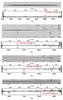 |
Fig. 3 Same as Fig. 2, for objects detected in the Ultra-Deep red and in the Deep datasets. |
| In the text | |
|
Fig. 4 top panel: for the full sample, the distribution of rest-frame EW if the lines are identified as Lyα (black histogram) or as [OII]3727 (red histogram). The filled histograms show objects without a detected continuum, for which the EW is a lower limit. lower panel: the same as the top panel, but for the 49 lines identified as ambiguous. The blue and green histograms represent respectively the rest-frame EW if the lines are identified as Lyα or as [OII]3727. |
| In the text | |
|
Fig. 5 Combined spectra for all serendipitous LAE in four redshift domains, centered on Lyα. The asymmetry of the line profile is clearly seen in each redshift range when comparing to a gaussian fit of the red wing of the line (long-dashed line). For each combined spectrum we report also the skewness calculated in the range 1201 < λ < 1231 Å. |
| In the text | |
|
Fig. 6 Combined spectra for 5.9 < z < 6.62. The top panel shows the continuum bluewards of the Lyα line. The bottom one focuses on the line, showing the asymmetric profile. The value for the skewness of the line is also reported. |
| In the text | |
|
Fig. 7 For each sub-dataset, we show the flux versus redshift together with the flux limit as a function of the redshift and wavelength (solid lines). The flux limit is empirically measured on the 2-d spectra. Filled and open circles represent respectively serendipitous Lyα galaxies and targets with Lyα emission. |
| In the text | |
|
Fig. 8 Completeness in line identification from Monte Carlo simulation as a function of the flux, for the three subsamples: Deep (solid line), Ultra-Deep red (dotted line) and Ultra-Deep blue (dashed line). |
| In the text | |
|
Fig. 9 Histogram of the percentage of recovered flux, for a set of a 3000 simulated lines randomly offset with respect to the center of the slit (solid line) and for the serendipitous lines (dotted line). The vertical lines show the median for the two distributions, around 55% of the recovered flux. The small inset shows the recovered flux as a function of the offsets for the simulated lines, for the 0.7, 0.9 and 1.2 arcsec FWHM lines (respectively in red, black and blue). |
| In the text | |
|
Fig. 10 Redshift distribution for the whole sample (black line), as well as for the different subsamples: solid lines show serendipitous lines, while dotted ones indicate primary spectroscopic targets; blue and red lines show the Ultra-Deep and deep subsamples, respectively. |
| In the text | |
|
Fig. 11 Full width half maximum (FWHM) distribution as measured from the CFHTLS images (top panel) and from the Lyα 2-d spectra (bottom panel). Targets are shown with a solid line, serendipitous objects with and without photometric counterparts are shown with a dotted and dashed line, respectively. The CFHTLS image used was built by stacking the 25% best-seeing exposures, and has a final PSF FWHM of about 0.5′′. In the top panel, we just show serendipitous objects with a photometric counterpart. |
| In the text | |
|
Fig. 12 Combined spectra of the serendipitous Lyα emitters, in several redshift ranges from z = 2 to z = 5.9. The displayed range of flux was selected to show faint continuum features, while the peak of the Lyα line is largely off-scale. Blue dotted lines indicate different spectral features depending on the redshift range: Ly-break at 912 Å, Lyβ at 1026 Å, OI at 1303 Å, CII at 1333 Å, SiIV at 1397 Å, CIV at 1549 Å, HeII at 1640 Å and CIII at 1909 Å. The horizontal dashed lines indicate the level of zero flux. |
| In the text | |
|
Fig. 13 Combined spectra of the target Lyα emitters in the redshift ranges 2 ≤ z ≤ 2.7 and 2.7 ≤ z ≤ 3.5. The displayed range of flux was select to show faint continuum features, while the peak of the Lyα line is largely off-scale. The horizontal dashed lines indicate the level of zero flux. |
| In the text | |
|
Fig. 14 UGR color–color plot for galaxies in our sample between 2.6 < z < 3.6. Filled and open circles represent respectively targets and serendipitous objects with optical counterpart. Black points show galaxies at all redshifts. The dashed box indicates the drop-out region in which galaxies at such redshifts are expected to lie. The cross in the bottom right part of the diagram shows the typical error bars. |
| In the text | |
|
Fig. 15 GRI color–color plot for galaxies in our sample between 3.6 < z < 4.2. Filled and open circles represent respectively targets and serendipitous objects with optical counterparts. Black points show galaxies at all redshifts. The dashed box indicates the drop-out region in which galaxies at such redshifts are expected to lie. The cross in the bottom right part of the diagram shows the typical error bars. |
| In the text | |
|
Fig. 16 Equivalent Width of the Lyα line as a function of the absolute magnitude at 1600 Å, for the objects with photometric counterpart, in three different redshift bins. Objects with detected continuum are shown as filled dots. Objects without a detected continuum, for which the equivalent width is only a lower limit, are shown as upperward arrows. The dotted line shows MUV = −21.5: objects brighter than this limit show a deficit of large equivalent widths (EW0 > 20). |
| In the text | |
|
Fig. 17 Luminosity versus equivalent width for the galaxies in our sample (red points); filled and open circles indicate respectively galaxies with and without a detected continuum. For the latter, the measure of the EW is a lower limit. Black diamonds, triangles, crosses and squares show respectively the samples of Ouchi et al. (2008), Dawson et al. (2007), Murayama et al. (2007) and Saito et al. (2008). |
| In the text | |
|
Fig. 18 LAE luminosity function in different redshift bins. No IGM absorption correction was applied here. Upper left, upper right and bottom left panels indicate 2 < z < 3.2, 3.2 < z < 4.55 and 4.55 < z < 6.6 respectively. The error bars reflect the Poissonian errors. Black points show literature data, spanning from z = 3 to z = 5.7: diamonds, triangles and squares represent Ouchi et al. (2008) at respectively z = 3.1, z = 3.7 and z = 5.7; asterisks, plus signs, crosses and circles indicate respectively Shimasaku et al. (2006) at z = 5.7, Murayama et al. (2007) at z = 5.7, Gronwall et al. (2007) at z = 3.1 and Dawson et al. (2007) at z = 4.5. We group together our measurements in the different redshift bins in the bottom right panel, to show that within the error bars, the Lyα LF does not evolve from z = 2.5 to z = 6. |
| In the text | |
|
Fig. 19 We report here our estimates of the intrinsic luminosity functions, corrected for the IGM absorption (shaded regions). Blue, green and red indicate respectively 1.95 < z < 3, 3 < z < 4.55 and 4.55 < z < 6.6 ranges. Solid lines show our best fits to the data. |
| In the text | |
|
Fig. 20 Evolution of the SFRD as a function of the redshift, inferred integrating the intrinsic Lyα luminosity functions down to 0.04 × L ∗ . Red open circles are our data, while blue and green open circles represent other Lyα SFRD respectively by Ouchi et al. (2008) and Gronwall et al. (2007). Open triangles, open squares, open lozenges, stars and crosses are UV estimates respectively by Schiminovich et al. (2005), Reddy et al. (2008), Bouwens et al. (2007), Beckwith et al. (2006), Tresse et al. (2007) and Bouwens et al. (2010). |
| In the text | |
Current usage metrics show cumulative count of Article Views (full-text article views including HTML views, PDF and ePub downloads, according to the available data) and Abstracts Views on Vision4Press platform.
Data correspond to usage on the plateform after 2015. The current usage metrics is available 48-96 hours after online publication and is updated daily on week days.
Initial download of the metrics may take a while.