| Issue |
A&A
Volume 634, February 2020
|
|
|---|---|---|
| Article Number | A97 | |
| Number of page(s) | 26 | |
| Section | Extragalactic astronomy | |
| DOI | https://doi.org/10.1051/0004-6361/201935400 | |
| Published online | 13 February 2020 | |
UV and Lyα luminosity functions of galaxies and star formation rate density at the end of HI reionization from the VIMOS UltraDeep Survey (VUDS)⋆
1
Aix Marseille Université, CNRS, LAM (Laboratoire d’Astrophysique de Marseille) UMR 7326, 13388 Marseille, France
e-mail: This email address is being protected from spambots. You need JavaScript enabled to view it.
2
University of Padova, Department of Physics and Astronomy, Vicolo Osservatorio 3, 35122 Padova, Italy
3
INAF – Osservatorio di Astrofisica e Scienza dello Spazio di Bologna, Via Gobetti 93/3, 40129 Bologna, Italy
4
Department of Physics, University of California, Davis, One Shields Ave., Davis, CA 95616, USA
5
European Southern Observatory, Avenida Alonso de Córdova 3107, Vitacura, 19001 Casilla, Santiago de Chile, Chile
6
INAF–IASF Milano, Via Corti 12, 20133 Milano, Italy
7
INAF, Osservatorio Astronomico di Roma, Monteporzio, Italy
8
Instituto de Investigación Multidisciplinar en Ciencia y Tecnología, Universidad de La Serena, Raúl Bitrán 1305, La Serena, Chile
9
Departamento de Física y Astronomía, Universidad de La Serena, Norte, Av. Juan Cisternas 1200, La Serena, Chile
10
Universitá di Bologna, Dipartimento di Fisica e Astronomia, Via Gobetti 93/2, 40129 Bologna, Italy
11
INAF – Osservatorio Astrofisico di Arcetri, Largo E. Fermi 5, 50125 Firenze, Italy
12
Astronomy Department, University of Massachusetts, Amherst, MA 01003, USA
13
Space Telescope Science Institute, 3700 San Martin Drive, Baltimore, MD 21218, USA
14
ESA/ESTEC SCI-S, Keplerlaan 1, 2201 AZ Noordwijk, The Netherlands
15
Leiden Observatory, Leiden University, PO Box 9513, 2300 RA Leiden, The Netherlands
16
Observatoire de Genève, Université de Genève, 51 Ch. des Maillettes, 1290 Versoix, Switzerland
17
Univ Lyon, Univ Lyon1, ENS de Lyon, CNRS, Centre de Recherche Astrophysique de Lyon UMR5574, 69230 Saint-Genis-Laval, France
Received:
5
March
2019
Accepted:
5
December
2019
Abstract
Context. The star formation rate density (SFRD) evolution presents an area of great interest in the studies of galaxy evolution and reionization. The current constraints of SFRD at z > 5 are based on the rest-frame UV luminosity functions with the data from photometric surveys. The VIMOS UltraDeep Survey (VUDS) was designed to observe galaxies at redshifts up to ∼6 and opened a window for measuring SFRD at z > 5 from a spectroscopic sample with a well-controlled selection function.
Aims. We establish a robust statistical description of the star-forming galaxy population at the end of cosmic HI reionization (5.0 ≤ z ≤ 6.6) from a large sample of 49 galaxies with spectroscopically confirmed redshifts. We determine the rest-frame UV and Lyα luminosity functions and use them to calculate SFRD at the median redshift of our sample z = 5.6.
Methods. We selected a sample of galaxies at 5.0 ≤ zspec ≤ 6.6 from the VUDS. We cleaned our sample from low redshift interlopers using ancillary photometric data. We identified galaxies with Lyα either in absorption or in emission, at variance with most spectroscopic samples in the literature where Lyα emitters (LAE) dominate. We determined luminosity functions using the 1/Vmax method.
Results. The galaxies in this redshift range exhibit a large range in their properties. A fraction of our sample shows strong Lyα emission, while another fraction shows Lyα in absorption. UV-continuum slopes vary with luminosity, with a large dispersion. We find that star-forming galaxies at these redshifts are distributed along the main sequence in the stellar mass vs. SFR plane, described with a slope α = 0.85 ± 0.05. We report a flat evolution of the specific SFR compared to lower redshift measurements. We find that the UV luminosity function is best reproduced by a double power law, while a fit with a Schechter function is only marginally inferior. The Lyα luminosity function is best fitted with a Schechter function. We derive a logSFRDUV(M⊙ yr−1 Mpc−3) = −1.45+0.06−0.08 and logSFRDLyα(M⊙ yr−1 Mpc−3) = −1.40+0.07−0.08. The SFRD derived from the Lyα luminosity function is in excellent agreement with the UV-derived SFRD after correcting for IGM absorption.
Conclusions. Our new SFRD measurements at a mean redshift of z = 5.6 are ∼0.2 dex above the mean SFRD reported in Madau & Dickinson (2014, ARA&A, 52, 415), but in excellent agreement with results from Bouwens et al. (2015a, ApJ, 803, 34). These measurements confirm the steep decline of the SFRD at z > 2. The bright end of the Lyα luminosity function has a high number density, indicating a significant star formation activity concentrated in the brightest LAE at these redshifts. LAE with equivalent width EW > 25 Å contribute to about 75% of the total UV-derived SFRD. While our analysis favors low dust content in 5.0 < z < 6.6, uncertainties on the dust extinction correction and associated degeneracy in spectral fitting will remain an issue, when estimating the total SFRD until future surveys extending spectroscopy to the NIR rest-frame spectral domain, such as with JWST.
Key words: galaxies: high-redshift / galaxies: evolution / galaxies: formation / galaxies: star formation / dark ages, reionization, first stars / galaxies: luminosity function, mass function
Based on data obtained with the European Southern Observatory Very Large Telescope, Paranal, Chile, under Large Program 185.A−0791.
© Y. Khusanova et al. 2020
 Open Access article, published by EDP Sciences, under the terms of the Creative Commons Attribution License (https://creativecommons.org/licenses/by/4.0), which permits unrestricted use, distribution, and reproduction in any medium, provided the original work is properly cited.
1. Introduction
As the first galaxies formed, they ionized the local medium they are embedded in, making radiation free to propagate (e.g., Dayal & Ferrara 2018). There is a growing consensus that the end of the Hydrogen reionization epoch is at a redshift z ∼ 6, stemming from several lines of evidence. The optical depth of HI reionization is one of many parameters in the standard ΛCDM cosmological world model and it can be measured from observations of the cosmic microwave background (CMB) power spectrum, giving access to the start, midpoint, and end of the reionization process (Hinshaw et al. 2013). These measurements can then be compared to the ionizing background output by observed populations of galaxies and active galactic nuclei (AGN). From the WMAP CMB observations, it has been inferred that the reionization would have been ∼50% completed at z ∼ 10.5 (Spergel et al. 2003). This would require a presence of a substantial ionizing background at quite early times, which should have materialized from star-forming galaxies at very early epochs. Early attempts to reconcile WMAP measurements with UV background estimates found it hard to identify enough galaxies capable of producing the required number of UV photons at early times (Robertson et al. 2013). Several hypotheses were proposed in order to solve this discrepancy, some among them invoking a substantial population of growing supermassive black holes and numerous faint galaxies escaping detection (Ciardi et al. 2003; Volonteri & Gnedin 2009).
The more recent findings on the epoch of HI reionization from the Planck experiment revisited the issue from the CMB point of view and significantly reduced the optical depth of reionization, which lowers the requirements on the number of ionizing photons and hence on the number of galaxies at high redshifts. Comparing the optical depth of reionization from Planck and from deep surveys, Robertson et al. (2015) and Bouwens et al. (2015b) claim that galaxies produce enough ionizing photons provided that there are enough faint galaxies populating the faint-end slope of the UV luminosity function. The latest results from the Planck experiment favor an even smaller reionization optical depth. The redshifts of the start, 50%, and end of reionization, derived from the CMB Planck maps with 95% CL, are now z = 10.4 ± 1.8, 8.5 ± 0.9, < 8.9, respectively (Planck Collaboration XLVII 2016). These results further consolidate the picture of reionization that happened late and fast, with reionization being driven by photons from massive stars in low mass galaxies as outlined in the 2018 Planck satellite results (Planck Collaboration VI 2018).
However, matching the CMB results with galaxy counts remains a considerable challenge. Deep galaxy surveys are constantly pushing the search for galaxies capable of producing the needed ionizing photons to higher redshifts and fainter luminosities (e.g., Le Fèvre et al. 2005, 2013, 2015; Scoville et al. 2007; Stark et al. 2009; Koekemoer et al. 2011; Pentericci et al. 2011; Ellis et al. 2013; Bowler et al. 2015; Bouwens et al. 2015b). The challenge is to characterize the luminosity function of these first galaxies with enough accuracy that the total number of ionizing photons can be accurately estimated. The census of high redshift galaxies is continuously improving, first and foremost on the basis of deep imaging with the Hubble Space Telescope (HST) and selected ground-based facilities. Faint multiband photometry reaching magnitudes AB ∼ 30 significantly increased the number of galaxy candidates with z > 6 and up to z ∼ 10, from the HST CANDELS (Grogin et al. 2011; Koekemoer et al. 2011), COSMOS (Scoville et al. 2007), Frontier Fields (Finkelstein et al. 2015; Lotz et al. 2017) and UltraVista surveys (McCracken et al. 2012). The additional boost from gravitational lensing allows to further constrain the faint-end slope of the luminosity function, reaching MUV ∼ −13 (Livermore et al. 2017; Bouwens et al. 2017; Ishigaki et al. 2018; Yue et al. 2018). These surveys form the basis of our understanding of the UV rest-frame luminosity function and the derived star formation rate density (SFRD, Madau & Dickinson 2014), at these redshifts. However, these observations remain challenging, and improving the faint galaxy census at z > 5 from high purity and completeness counts of galaxies with confirmed redshifts, therefore, remains of the utmost importance, particularly with regard to setting robust constraints on the SFRD history.
In this paper, we focus on providing robust counts of galaxies covering a redshift range from z ∼ 5 to z ∼ 6.6, a time close to, or including, the end of reionization. This corresponds to a cosmic time period from 0.8 to 1.15 Gyr after the Big Bang. We base our counts on a sample of galaxies with a reliable spectroscopic redshift identification obtained from the VIMOS UltraDeep Survey (VUDS, Le Fèvre et al. 2015), at variance from most previous studies based on photometric redshift identification (McLure et al. 2009; Bouwens et al. 2015a; Bowler et al. 2015) or spectroscopy with narrower selection criteria (Ouchi et al. 2008; Cassata et al. 2011; Santos et al. 2016; Drake et al. 2017). We identify and characterize star-forming galaxies, focusing on several key quantities, including the UV rest-frame luminosity, the Lyα line luminosity, as well as stellar mass, star formation rates (SFR), and other parameters derived from the spectral energy distribution (SED) fitting. We derive cosmic SFRDs from observed rest-frame UV luminosity functions, as well as from Lyα luminosity functions.
The paper is organized as follows. In Sect. 2, we describe our methods to isolate a reliable sample of 49 galaxies with spectroscopic redshifts 5 < z < 6.6. We present the sample in Sect. 3, including the redshift distribution, average spectral properties, UV β-slopes, and the distribution of these galaxies in the SFR versus stellar mass diagram. Observed galaxy counts are used with UV and Lyα luminosities to derive luminosity functions in Sect. 4. We then derive SFRDs from the UV and Lyα luminosity functions, compare them, and discuss their evolution with redshift in Sect. 5. The results are summarized in Sect. 6.
Throughout the paper we use ΛCDM cosmology with H0 = 70 km s−1 Mpc−1, ΩΛ = 0.70, Ωm = 0.30. All magnitudes are given in the AB system.
2. Data
2.1. Spectroscopic and photometric data
We used the spectroscopic sample of galaxies drawn from VUDS, which is described in detail in Le Fèvre et al. (2015). The wavelength coverage of the survey is from 3650 to 9350 Å, making it possible to obtain secure redshift measurements up to redshift z∼6.6, at which the Lyα–1215 Å line leaves the spectral window. The spectroscopic redshifts in VUDS are measured based on several spectral features with accuracy of dz ∼ 10−3 (Le Fèvre et al. 2015). Most of the spectra in the survey were observed with a low-resolution grating of VIMOS spectrograph (R = 230). Complementary to it, a number of objects were observed with a medium resolution of R = 580. The targets with zphot > 4.0 had a higher priority to be observed with a medium resolution.
The survey covers three different fields with a total area of 1 deg2: VVDS02h, COSMOS, and ECDFS. This minimizes the effects of cosmic variance. A wide range of ancillary data is available for each field to produce a sample, for which completeness and purity are well controlled, and to infer physical parameters, most importantly stellar masses and SFRs through SED fitting performed with the knowledge of the accurate redshift.
In the VVDS02h field, we used photometry from the 7th data release of CFHT Legacy Survey (CFHTLS, Cuillandre et al. 2012), which covers the u*, g′, r′, i′, z′ optical bands. It is complemented by the infrared data in J, H, and K bands from WIRCam Deep Survey (WIRDS, Bielby et al. 2012), and in two IRAC bands (3.6 and 4.5 μm) from the Spitzer Extragalactic Representative Volume Survey (SERVS, Mauduit et al. 2012).
The full range of photometric observations in the COSMOS field is presented on the COSMOS web site1. In this work, we use the optical data from CFHT for u* band, Subaru broad bands (B, V, g+, r+, i+, z+), the near-infrared bands J and K from UltraVista (McCracken et al. 2012), and IRAC bands from the Spitzer Extended Deep Survey (SEDS, Ashby et al. 2013).
In the ECDFS field, we used depending on availability either the CANDELS set of photometry (Grogin et al. 2011; Koekemoer et al. 2011), which includes observations in the optical and near-infrared HST bands, or the Taiwan ECDFS Near-Infrared Survey data (TENIS) with observations in J and Ks bands (Hsieh et al. 2012) complemented by the Galaxy Evolution from Morphology and SEDs survey (GEMS) in F606W and F850LP bands (Caldwell et al. 2008).
The main target selection was based on photometric redshifts and was designed to go to the highest possible redshifts starting from z = 2. The galaxies were chosen to have zphot + 1σ ≥ 2.4, where zphot is either the first or the second peak in the photometric redshift probability distribution function (PDF). The limiting magnitude of the main survey target selection is i = 25. This primary sample was complemented by galaxies chosen with two widely used techniques. The first one is the Lyman-break or dropout technique, which is based on the search of a break in the continuum corresponding to the changing spectral shape of a galaxy continuum between the Lyman limit at 912 Å and Lyα, classically followed in color-color diagrams (Steidel et al. 1996). The second technique is based on the search of Lyα emission line in narrow bands at 814 nm and 921 nm corresponding to z ∼ 5.7 and 6.57, respectively (Taniguchi et al. 2005). The galaxies from both these selections may have i > 25. The galaxies chosen with the dropout technique have limiting magnitude KAB ≤ 24 and were added to the target sample only if they are not already selected in the primary sample. In our high redshift sample, we have about 10% of the sample chosen by these criteria.
In addition to this main sample, in the process of examining all 2D spectra visually, the VUDS team discovered a number of single emission lines belonging to objects falling by chance in the slits, but for which no counterparts could be identified on any of the available images. These were analyzed following a method similar to that of Cassata et al. (2011) to assess the nature of the line. In this way, we identified a number of serendipitous Lyα emitters (LAE) with a UV continuum flux too faint to be detected in broad photometric bands.
The combination of these samples assembled from complementary selection functions resulted in a high redshift sample covering a broad range of properties. The selection function of the sample is well-defined and makes it possible to accurately derive volume-average quantities, such as luminosity functions. The selection of each subsample needs to be fully taken into account in determining luminosity functions because the galaxies chosen by different techniques were drawn from different parent populations, as discussed in Sect. 4.
Spectroscopic redshifts were measured with standard cross-correlation of a spectrum with reference galaxy spectra using the EZ tool (Garilli et al. 2010). The adopted redshift reliability flags are described in Le Fèvre et al. (2015). In short, these were obtained from visual estimates of the redshift measurement reliability from several observers, based on several indicators including the signal-to-noise ratio (S/N) of the spectral continuum, the number of matching emission and/or absorption lines, the strength of the cross-correlation peak, etc. The following probabilities to be correct were determined for each of the flags after repeat and independent observations of a subsample of galaxies in the survey: 50−75%; flag 2: 75−85%; flag 3: 85−95%; flag 4: 95−100%; flag 9: ∼80%.
Spectroscopic redshift measurements using the observed spectral range 3650−9350 Å are challenging at z > 5 since the faint fluxes of the continuum and emission lines are detected against the bright Earth atmosphere emission. Even with 14 h integrations with VIMOS on the 8 m ESO-VLT, a high fraction of galaxies still has insecure redshifts with reliability flag 1 at these redshifts. Another challenge is the possible confusion between the Lyα and [OII] emission lines due to the resolution of our spectra. The [OII] doublet or an asymmetric structure of Lyα line are not resolved on the spectra of individual objects at the observed spectral resolution. Therefore, additional verification of measured redshifts was necessary. We scrutinized each of the z > 5 candidates following a clear reference protocol to further assess the reliability of their redshifts. This procedure is described in Sect. 2.2.
We extensively used the ancillary data, such as multiband deep imaging and photometry. With direct image examination, we identified cases, in which spectra belonged to two close companions at different redshifts. We then attempted to disentangle true high redshift object from the low redshift interloper combining the spatial location of spectral features observed on the 2D spectrograms with the location of objects observed in images in different wavebands (e.g., indicating a possible continuum dropout signaling a Lyman break for one of the objects).
We also used the photometric measurements to perform SED fitting of each candidate galaxy, with and without fixing the redshift. The SED fitting without fixing the redshift provided us with the PDF of photometric redshifts and the best fit template at the peak of this PDF. In order for the SED fitting to be helpful in distinguishing between the true high redshift galaxies and low redshift interlopers as described in Sect. 2.2, we used a wide range of templates, suitable for both high and low redshift. We used Bruzual & Charlot (2003) models with Chabrier (2003) initial mass function, two star formation histories: exponentially declining and delayed, and solar and subsolar metallicities (Z = 0.02 and Z = 0.008) to fit the SED with LePhare (Arnouts et al. 2002; Ilbert et al. 2006). We considered two extinction laws: Calzetti et al. (2000) and SMC-like (Prevot et al. 1984), and a range of the E(B − V) values from 0.0 to 0.5. The best fit was determined by the minimization of χ2.
The SED fitting using the fixed spectroscopic redshift delivered the best estimates of physical parameters and the best fit template at the spectroscopic redshift. We defined the uncertainties on physical parameters from the PDF of each parameter. We used the uncertainties of the apparent magnitudes used for SED fitting to robustly determine the uncertainty of the FUV magnitude measurements (see Sect. 4.2).
In Sect. 3, we extend up to z = 6.6 the work of Tasca et al. (2015), which was done up to z = 5.5. When comparing different physical parameters and their evolution with redshift, we used consistent methods.
2.2. Cleaning of the high redshift sample
We started by selecting all galaxies from VUDS with spectroscopic redshifts in our range of interest 5.0 < z < 6.6. We selected 111 candidates with all reliability flags. Seven of these candidates had the most secure redshifts with flags 3 or 4. In most of the spectra, however, the observed features were either one emission line, which was associated to Lyα in the redshift measurement process, or a continuum break, which was associated to the break at 1215 Å produced by the strong intergalactic medium (IGM) extinction at these redshifts (e.g., Thomas et al. 2017a). Up to redshift 5, we could usually distinguish between Lyα and [OII] emission lines because Hβ and the [OIII]–4959/5007 Å doublet would still be observed in the VIMOS spectral window if a single line with λ < 7200 Å was [OII]–3727 Å rather than Lyα. At the higher redshifts considered in this paper, Hβ and [OIII] would be shifted beyond the observed wavelength range and, therefore, the detection of a single emission line with λ > 7200 Å should be interpreted with caution. Another degeneracy in redshift measurement comes from the possibility to misinterpret a Balmer break at ∼4000 Å in a spectrum as a Lyman break or dropout in the continuum due to the absorption by the neutral gas along the line of sight. These degeneracies impose that each high redshift galaxy candidate has to be scrutinized to identify possible low redshift galaxies contaminating our sample. To resolve this issue, we made use of all spectroscopic and photometric data and inspected each galaxy individually imposing several criteria for a galaxy to be retained in the final 5.0 < zspec < 6.6 sample:
1. No detection in photometric bands corresponding to wavelengths below the Lyman limit at 912 Å, as neutral gas in the galaxy itself should not let photons out;
2. No detection or weak detection below the 1σ limit in photometric bands corresponding to wavelengths 912 Å < λ < 1215.7 Å, as neutral gas in the intervening IGM should absorb most of the photons emitted by the galaxy (depending on the line of sight; Thomas et al. 2017a);
3. At least one detection in a photometric band corresponding to the rest-frame 1215.7 Å (for LAE) or at wavelengths longer than 1215.7 Å for galaxies without Lyα in emission, as some continuum photons should be detected;
4. The difference between spectroscopic and photometric redshifts should be zspec − zphot ≤ 3σ, with σ being the halfwidth of the 68.3% confidence interval around the peak in the photometric redshift PDF, for at least one of the peaks in the photometric redshifts PDF2;
5. The best SED fit template with the redshift fixed at the spectroscopic redshift and based on photometric points only is in agreement with the observed spectrum, including features expected to be observed in the spectrum (e.g., main spectral lines, continuum shaped like a break at around Lyα or at the Lyman break).
Galaxies with redshift reliability flags 1 and 9 will be affected the most by the degeneracies described above; as for flag 1, these spectra have generally low S/N and correspond to the faintest galaxies. The spectra with flag 9 have only a single feature identified in the spectrum – emission line (presumably Lyα). To be retained in our final sample, these galaxies, therefore, had to pass all the above criteria. The galaxies with reliability flags 2−4 have a higher probability to be correct and, therefore, we excluded them from the final sample only if they did not pass more than one of the above criteria.
This procedure was motivated by the fact that various effects could affect the photometry of the galaxy. The spectroscopy of each galaxy should, therefore, remain the primary source of information. We paid special attention to the following cases. First of all, if the PDF was very wide, it was not possible to have a robust estimate of the photometric redshift. In this case, we trusted the spectroscopic redshift (this is the case for six galaxies in the sample). Next, in the presence of bright nearby objects, the sky subtraction could be unreliable. The broad band magnitudes for the faint objects were highly uncertain in that case and the photometry could be misleading. The same goes for the cases, where the foreground object along the line of sight was blend with the high redshift candidate, or when the image was affected by artifacts from the image processing. Finally, we found evidence that one of the observed object is an AGN (this object has a broad Lyα emission line) and, therefore, can be variable.
Together with the spectra (1D and 2D), photometry, and SED of each galaxy, we analyzed all the images and looked for the evidence of such effects. If the 2D spectrum and the images were consistent with the galaxy being at high redshift, but some evidence for contamination was found, we kept it in our sample. The photometry of this galaxy should, however, be used with caution. Such an example is shown in Fig. A.1 where the high redshift object is close to a foreground object affecting both the photometry and spectrum.
In Table A.2, we present a summary of the selection criteria for each galaxy. We found six galaxies, which have zspec − zphot > 3σ. Three of them show signs of contamination by nearby objects, and two have very narrow peaks in PDF, which are 3σ to 6σ away from the spectroscopic redshift, but the best fit template to the photometric redshift cannot explain the observed spectrum. We, therefore, kept these galaxies with their spectroscopic redshift. We also retained two galaxies with faint detections below 912 Å in the final sample since they have reliable spectroscopic redshifts and SED fitting clearly points to the same redshift as spectroscopy, while the detections below 912 Å are likely to be spurious.
The criteria above helped us to efficiently get rid of low redshift interlopers, as well as to analyze the reliability of the photometry, which we used later to derive FUV-fluxes and physical properties.
Other possible contaminants of our sample are late-type stars (e.g., late M-types or brown dwarfs). When we measured redshifts with EZ, we used a library of star and galaxy templates to fit the observed spectrum by chi-square minimization algorithm. If we only observed continuum in spectra without emission lines, we compared best fit with a star template with the best fit from galaxy templates. If no star template was able to reproduce the observed spectrum better than the galaxy template, we saved the object in our sample. Otherwise, we concluded that the observed object is a star.
During the inspection of the spectra, we found one quasar with a broad Lyα line (FWHM ∼ 4300 km s−1) at redshift of z = 5.472. We used the luminosity function of McGreer et al. (2018) to estimate the probability of finding quasars in our sample. We integrated the luminosity function down to MFUV = −21.4 (the range of absolute magnitudes corresponding to completeness limits of the parent catalog of our sample) and obtained the quasar number density. We then multiplied it with the average target sampling rate and the comoving volume of the survey area between the redshift limits z = 5.0 and 6.6, assuming for simplicity a 100% detection probability over the full redshift range (this assumption can lead to overestimation of the real probability to find quasars but it is safe to use in defining an upper limit). Assuming Poisson distribution, we found that the probability of finding more than one quasar is less than 0.7%, and the probability of finding one is 11%. Therefore, in the observed range of absolute magnitudes, we expect to have a clean sample of only star-forming galaxies after excluding this quasar discovered in the sample.
We could not apply the above-described criteria to the galaxies with a single emission line and without a photometric counterpart or with contaminated photometry. We, therefore, needed a different way of investigating the reliability of their redshifts. One of the arguments in support of observing Lyα is the skewness of the emission line. We defined the skewness as a normalized third moment of the flux distribution in the line (see Eq. (1) in Kashikawa et al. 2006). The Lyα line has an asymmetric shape with positive skewness due to radiation transfer effects, while the unresolved [OII] doublet is usually symmetric with a skewness close to zero (Kashikawa et al. 2006; Cassata et al. 2011). Another effect at high redshift comes from the IGM and circumgalactic medium (CGM), which absorb the continuum below Lyα. Due to this effect, the Lyα line becomes even more asymmetric.
These effects are difficult to observe on a single low signal-to-noise spectrum at the observed spectral resolution, but the structure of the emission line is visible on the stacked spectra. We show in Fig. 1 the stacked spectrum around Lyα of LAE from our sample (see Sect. 3.1 for details). We clearly see that the continuum at wavelengths bluer than Lyα is completely absorbed by IGM and CGM, and the shape of the line is asymmetric.
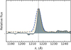 |
Fig. 1. Stacked spectrum of 36 galaxies with Lyα in emission. The solid line and shaded area is the observed spectrum, the dashed blue line is a Gaussian, fitted to the red wing of the emission line. The orange dotted line is the line spread function. The vertical dashed line indicates the position of Lyα line λ = 1215.7 Å. |
The measured skewness of the line is SK = 2.05. Therefore, the line is consistent with being Lyα and cannot be associated to [OII]. This value is higher than the value from Cassata et al. (2011) reporting SK = 1.73 for redshifts 4.6 < z < 5.9, but is consistent with expectations for higher redshifts of our sample, where the IGM absorption would be higher. Cassata et al. (2011) report a value SK = 2.02 for 5.9 < z < 6.6 (measured from only six galaxies). This is comparable with our result within uncertainties. The fact that the stacked spectrum of our galaxies has a very strong skewness gives further confidence that our sample is free from the contamination of low redshift objects.
3. Final sample of 5.0 < z < 6.6 galaxies
After the procedure described above, we obtained a sample of 49 galaxies with secure spectroscopic redshifts, 8 of them observed with a medium resolution.
The redshift distribution of the sample is shown in Fig. 2. The median redshift is z = 5.59. For 32 of them, we derived physical properties and FUV magnitudes from ancillary photometric data (the wavelength coverage does not allow us to measure FUV flux from spectra). In the subsections below, we describe the average and individual properties of the galaxies in our sample.
3.1. Average spectral properties
The 1D spectra of the individual galaxies together with the best fit SED template and images can be found in the appendix. We present the 2D spectra ordered by redshift in Fig. 3.
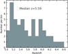 |
Fig. 2. Redshift distribution of our sample. |
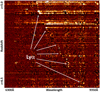 |
Fig. 3. 2D spectra of VUDS galaxies with 5.0 ≤ z ≤ 6.6, ordered by redshift. The spectral range covers from 6300 to 9350 Å following the spectral region around Lyα. Lyα appears in emission or in absorption depending on spectra. |
We present median stacked spectra of galaxies in our sample, normalized on the continuum at 1400 Å rest-frame and with equal weight to reflect the average stellar population. We stacked two groups of galaxies observed with low resolution: galaxies with Lyα in emission (Fig. 4) and Lyα in absorption (Fig. 5). The continuum was detected in both cases without significant emission below the Lyman limit at 912 Å, an indication that our sample selection and subsequent screening for low redshift interlopers was efficient in keeping only objects at 5.0 ≤ z ≤ 6.6. The stack of emission line galaxies corresponds to galaxies with a median MFUV = −20.50 fainter than for the absorption stack with a median MFUV = −20.78 (for galaxies with unknown FUV-magnitude an upper limit of −19.0 was used). The most prominent line in both cases is Lyα with equivalent width EW0(Lyα)≃ − 100 Å in the emission spectrum (negative values of EW correspond to emission lines, positive to absorption), and EW0(Lyα)≃5 Å in the absorption spectrum. There are only weak traces of absorption lines in the stack of Lyα emitting galaxies, while on the stack of spectra with Lyα absorption, the absorption lines are more prominent thanks to the brighter FUV continuum. In particular, the Lyman series (Lyγ − 972 Å, Lyβ − 1026 Å and Lyα − 1215 Å), as well as absorption lines (SiII–1260 Å, OI–1303 Å CII–1334 Å, and SiIV–1394 Å) are well seen on the stacked spectra. We defer the comparison of the spectral properties of star-forming galaxies at z ∼ 5.6 to the properties at lower redshifts to a future paper.
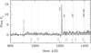 |
Fig. 4. Median stack of 36 spectra at 5.0 ≤ z ≤ 6.6 (median z ∼ 5.6) with Lyα in emission. |
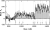 |
Fig. 5. Median stack of 11 spectra at 5.0 ≤ z ≤ 6.6 (median z ∼ 5.6) with Lyα in absorption. |
3.2. UV-continuum slopes
We explored three methods of measuring UV-continuum slopes β: a power law fλ ∼ λβ (e.g., Meurer et al. 1999) fit to the region from 1490 Å to 2350 Å on the best fit SED template, a fit to the photometric points corresponding to the same region (if available) or a fit to the spectrum in the region observed after Lyα (if the UV continuum is observed with S/N > 1). The results are consistent within the errors (see Fig. 7).
In Fig. 6, we show the relation between the UV-continuum slopes β and the rest-frame FUV absolute magnitudes for galaxies (both measured from SED fitting). We observe a decrease in the biweight mean β with MFUV, similar to the results of Bouwens et al. (2014). We note, however, that most of the β measurements lay below the average values of Bouwens et al. (2014) at z = 4 and z = 5. This indicates that the galaxies in our sample are on average less dusty than Lyman-break galaxies (LBGs) at z < 5, although the results of Castellano et al. (2012) at z ∼ 4 have steeper slopes and are in a better agreement with our results. For MFUV > −22, we observe a steepening of the continuum slopes to fainter FUV magnitudes with a similar slope as in Bouwens et al. (2014).
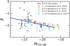 |
Fig. 6. β-slope vs. FUV-magnitudes of our sample. Gray circles indicate the individual measurements for the galaxies with most reliable photometry, and gray crosses for the remaining ones. Blue circles are biweight means in bins of 0.7 mag size. The straight blue line is the linear fit to the biweight mean values. The colored crosses are values from Bouwens et al. (2014) and Castellano et al. (2012) at different redshifts. |
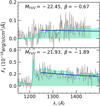 |
Fig. 7. Spectra of UV bright galaxies with flat and steep UV-continuum slopes (id = 528295041 and id = 520180097 at z = 5.487 and 5.1378, respectively). The rest-frame spectra are plotted in gray and the best SED template in light green. The solid blue line shows our fit to the continuum on spectra. |
At the brightest magnitudes, however, we observe a larger scatter and a possible change of this behavior with some galaxies appearing bluer with very steep (negative) β slopes. In the same bin, we also observe a galaxy with the reddest color in our sample and flat β slope. This galaxy is shown in Fig. 7. It has robust measurement of β = −0.56 ± 0.05 from the photometric fit (β = −0.67 ± 0.23 from the fit to spectroscopic data). This galaxy, therefore, is not an outlier. We conclude that the scatter of β is large in this bin. The brightest galaxies in this redshift range seem to be diverse in their spectral slopes, which may indicate different dust properties. The properties of galaxies depend on their age: the oldest galaxies had enough time to build up dust and appear redder in their continuum, while younger, recently formed galaxies lack dust and appear bluer.
3.3. Main sequence of star-forming galaxies and sSFR at z ∼ 5.6
The distribution of galaxies in the SFR-stellar mass diagram is shown in Fig. 8. SFR and stellar mass are tightly correlated over the stellar mass range 9 < log Mstar/M⊙ < 10.5, showing the existence of the “main sequence” of star-forming galaxies at 5 < z < 6.6 (e.g., Elbaz et al. 2007; Whitaker et al. 2012, 2014; Tasca et al. 2015; Salmon et al. 2015; Santini et al. 2017; Pearson et al. 2018). We fitted the distribution with a simple power law and found that  with α = 0.85 ± 0.05 at z ∼ 5.5 and with a scatter around the relation of ∼0.13 dex.
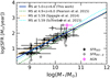 |
Fig. 8. SFR–M* diagram of our sample. The solid blue line is the fit to our data, representing the main sequence of star-forming galaxies at these redshifts. The dotted cyan, orange, and green lines are extrapolations of the main sequence at our median redshift from Speagle et al. (2014), Schreiber et al. (2015), Pearson et al. (2018). Filled circles are galaxies with reliable photometry and open circles are galaxies with possible contamination from bright nearby objects. The magenta diamond is the AGN identified in our sample. The gray diamonds are estimations of SFRs from the FUV magnitudes using IRX–β relation. |
The low dispersion in the Mstar − SFR relation that we observe may result in part from using spectroscopic redshifts rather than less precise photometric redshifts as used in most other studies (with typical errors δz ∼ 0.3 at these redshifts). It may also be the result of the method used to derive Mstar and SFR from the SED fitting, as masses and SFRs were not derived independently, even if we used a broad range of SED models (Sect. 2.1). Obtaining independent estimates of the SFR with the data in hands is difficult, but we made an attempt using UV-luminosities with the standard Kennicutt relation (Kennicutt 1998) together with the IRX–β relation to account for dust attenuation following Meurer et al. (1999). Both SFR-estimates are fairly consistent with each other. We find a similar main sequence relation, but with a larger scatter around the main sequence of 0.34 dex. However, in this case, the SFR is affected by uncertainties on the dust correction, which may not follow the Meurer et al. (1999) relation at high redshifts (Narayanan et al. 2018, and references therein). More robust estimates of the SFR could possibly be obtained by combining UV and IR luminosities, but this is beyond the scope of this paper and will be discussed in a future paper.
Previous studies show that the main sequence has a turnover at higher masses. This was observed at z ∼ 2. At higher redshifts, however, the turnover becomes less prominent (e.g., Whitaker et al. 2014; Tasca et al. 2015; Santini et al. 2017; Pearson et al. 2018). We show in Fig. 9 the median SFRs of galaxies in different mass bins for redshift ranges from 0 to 6.6 from VUDS. The data for z < 5.5 is taken from Tasca et al. (2015), and the data in the last redshift bin 5.5 < z < 6.6 is from this work. Since we used consistent methods to derive SFRs and stellar mass, we are able to extend the previous results from VUDS to higher redshifts.
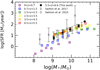 |
Fig. 9. Main sequence of VUDS galaxies at different redshifts. The colored squares show the median SFR in mass bins from Tasca et al. (2015). The black circles are median SFRs from this work at 5.5 < z < 6.6. |
The turnover of the main sequence is clearly seen at z < 3.5, but it seems to disappear at higher redshifts. Essentially all our galaxies lay very close to a linear main sequence suggesting that the majority of them are still star-forming. In our redshift range, we do not observe a significant turnover at high mass in the main sequence, as would be expected if star-formation in massive galaxies was starting to be quenched. However, we find that a few individual galaxies are slightly below the main sequence at masses log M*/M⊙ > 10.3. The uncertainties on the stellar masses and SFRs of these galaxies and their small number, however, do not allow us to draw any firm conclusions about their nature and a possible start of quenching processes.
We then measured the specific star formation rate (sSFR) in the 5.0 < z < 6.6 redshift range. It was previously shown that the sSFR evolution with redshift is slower at z ≳ 2.4 (Tasca et al. 2015; Faisst et al. 2016). We computed the median sSFR of our sample using a lower stellar mass limit of M* > 1010 M⊙. We found logsSFR(Gyr−1) = − 8.37 ± 0.08 and −8.46 ± 0.09 at 5.0 < z < 5.5 and 5.5 < z < 6.6, respectively. SSFR in our highest redshift bin is only slightly higher than logsSFR(Gyr−1) = − 8.46 ± 0.06 found by Tasca et al. (2015) at 4.5 < z < 5.5. We conclude that the sSFR evolution continues to flatten with redshift up to z ∼ 6.6.
Our results are shown in Fig. 10. Over the redshift range of our sample, they are in excellent agreement with the latest results from HST Frontier Fields (Santini et al. 2017), with semi-analytical models based on gas accretion via cold streams (Dekel et al. 2009) and with the Gadget-2 and Illustris numerical simulations (Davé et al. 2011; Sparre et al. 2015). The simulations, however, do not show any change in the sSFR evolution at z ∼ 2.5, contrary to what is observed: a fast increase with redshift at z < 2.5 and a slower increase at z > 2.5. More work needs to be done to infer, which processes are driving the evolution of the sSFR through cosmic time.
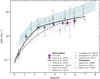 |
Fig. 10. Redshift evolution of the sSFR. Results of various observations and numerical simulations are shown. The magenta star shows the result of this work, an extension of Tasca et al. (2015) work (light blue stars). The solid line shows the fit to the previous results from VUDS (Tasca et al. 2015), the shaded area and the dashed line shows the results, coming from the observations of EW(Hα) in COSMOS (Faisst et al. 2016). |
We note that our SFR estimates are based on rest-frame UV and optical. If a significant fraction of the star formation is hidden by dust at redshifts z ∼ 5−6, then our measurements may underestimate the total SFR. Observations of the dust-obscured star formation from the far-infrared are necessary to quantify this and will be discussed in a future paper.
3.4. Age and formation redshift distribution
Another property that can be inferred from the SED fitting is the age of the dominant stellar population(s). We followed Thomas et al. (2017b) to compute ages, defined as the timespan since the onset of star formation. Ages were derived from fitting a broad range of SED templates to the combination of the spectra and photometry, using exponentially delayed star formation histories; see Thomas et al. (2017b) for more details. The median age of galaxies in the sample is 0.35 Gyr and the redshift of formation varies from z = 5.5 for the youngest galaxies at z ∼ 5 to z = 10.7 for the oldest galaxies at the highest redshifts. Over 90% of the galaxies in our sample have a redshift of formation z > 6.0 and, therefore, might have contributed to the reionization of the Universe, if they had non-negligible Lyman continuum escape fractions.
4. Luminosity functions
4.1. 1/Vmax method
We used the 1/Vmax method (Schmidt 1968) to determine luminosity functions. Since we were using a spectroscopic survey, we had to take into account that only a fraction of the galaxies in the field was targeted by the spectrograph (target sampling rate, TSR) and that for only a fraction of these galaxies, a redshift has been measured (spectroscopic success rate, SSR). We, therefore, weighted each galaxy as
 (1)
(1)
The TSR is defined as the ratio of galaxies targeted in the survey to the underlying population of galaxies for each of the selection criteria used (Sect. 2.1), which is known from the parent photometric catalog. Since different priorities were given to targets depending on the redshift (Sect. 2.1), the TSR is different depending on the redshift range. We evaluated the TSR and SSR for the redshift range discussed in this paper.
The parent population of galaxies is well known for magnitudes i < 25 from the parent catalog (the catalog is complete at these magnitudes). At fainter magnitudes, we needed to take into account the magnitude incompleteness in the parent catalog. We applied additional completeness corrections (Ccorr) using the ratio of Ncat/Nexp, where Ncat is the number of galaxies in the parent catalog, and Nexp is the expected number of galaxies at fainter magnitudes if the catalog was complete. To evaluate Nexp, we used the i-band magnitude distribution in the photometric catalog and assumed that the number of faint galaxies continues to increase at i > 25. This correction is shown in Fig. 11. The weights for faint galaxies were then calculated as 1/(TSR * SSR * Ccorr). We note that due to these additional corrections, the data on the faint end of luminosity functions should be interpreted with caution.
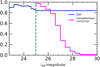 |
Fig. 11. SSR as a function of i magnitude and the corrections applied to TSR at magnitudes i > 25, below the completeness limits. |
The underlying parent population of serendipitous galaxies is not known. We assumed that all faint galaxies, which fall on the slit area serendipitously, were observed and we estimated the TSR of this population as the ratio of the area covered by slits to the whole observed area, which is equal to ∼0.2%. A few galaxies with i > 25 from the parent catalog were also observed if they fell by chance into the slits. We treated them as serendipitous and used the same TSR. All TSR used in this paper are shown in Table 1.
Target sampling rates of different selection criteria.
We used galaxies with all reliability flags, which were confirmed with a redshift in the range of interest following the criteria in Sect. 2.2. The SSR is, hence, the ratio between the number of galaxies with a confirmed redshift to the number of observed galaxies. The SSR should not depend on the selection criteria, but it depends on the i-band magnitude since brighter galaxies have a higher S/N of continuum detection enabling easier redshift measurement. We evaluated SSR for the whole sample of galaxies with i < 25 as a function of magnitude. The SSR of fainter galaxies is more uncertain as it starts to depend on the strength of the Lyα line, rather than on the brightness of the continuum. Indeed, the strong LAE have fainter FUV-continuum, but higher probability to be detected. We, therefore, ignore the dependence on i-band magnitude for the fainter subsample and assume a constant SSR based on Lyα emission detection limits. The resulting SSR is shown in Fig. 11.
After assigning the TSR and SSR as described above, we determined the luminosity function as
 (2)
(2)
where M is the FUV magnitude or the Lyα luminosity in log, ϕ(M) is the number density in magnitude or luminosity bin, dM is the bin size, Ngal is the total number of galaxies, and Vmax, i is the maximum comoving volume where the ith galaxy can be observed. We determined the volume Vmax, i using the i magnitude for the main photo-z selected sample, K-magnitude for the color selected sample, and the flux of Lyα line for the remaining galaxies.
We estimate the uncertainties of our results assuming Poisson distribution of the number counts and taking into account the weights associated with each galaxy. Since the weights themselves have uncertainties, we calculated the luminosity function using the upper and lower limits of the weights, which are defined by the estimated errors on the weights.
4.2. UV luminosity function
Before determining the UV luminosity function, we investigated how uncertainties of the observed magnitudes propagate into the uncertainty of FUV magnitudes determined with LePhare. We took a set of observed magnitudes of each galaxy and then sampled 500 new magnitude sets, assuming Gaussian errors on the measured flux. We used these magnitude sets to recompute the absolute magnitude using the same method and compared the new values with the  (the initial and the best estimate of the absolute magnitude of a galaxy). We obtained in this way the distribution of ΔMFUV for each individual galaxy.
The inspection of these distributions shows that galaxies with the smallest number of photometric detections (2−3) have the largest uncertainties on MFUV. These galaxies were only detected in the bands where the emission lines are located, such as the i-band or z-band for Lyα and IRAC bands for [OIII] and Hα lines. Therefore, for these galaxies, the estimation of MFUV strongly depends on the assumptions made about the strength of the emission lines. We introduced these galaxies into the luminosity function by weighting them with the probability for each of them to be inside each absolute magnitude bin. To compute this probability, we normalized the distribution of ΔMFUV, obtaining the probability distribution of the absolute magnitude and integrated this distribution between the bin limits.
Although the distribution of ΔMFUV varies slightly from galaxy to galaxy, the average uncertainty remains almost the same for a given photometric set used, which is different depending on the field (as discussed in Sect. 2). The average uncertainties are 0.07, 0.04, 0.05 for COSMOS, VVDS02h and ECDFS fields respectively. For a few galaxies in ECDFS field with photometry from TENIS, the average uncertainties are larger (∼0.14), due to a small number of bands.
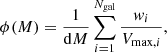
After examining the quality of MFUV magnitudes, we proceeded to determine the UV luminosity function of our sample. We present our results in Fig. 12 and Table 2. We compare our results with luminosity functions reported in the literature at z = 5 and z = 6 (McLure et al. 2009; Bouwens et al. 2015a; Bowler et al. 2015) and find a good agreement within error bars with our luminosity function being closest to the z = 5 luminosity function of Bouwens et al. (2015a).
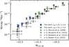 |
Fig. 12. UV luminosity function at the median redshift z = 5.6. The blue stars are UV luminosity function estimations drawn from the bright i < 25 sample, the green stars are from the faint sample with completeness correction as described in Sect. 4.1. The black open symbols are UV luminosity function from the literature at z ∼ 5 and the gray ones at z ∼ 6. |
UV and Lyα luminosity function measurements.
Bowler et al. (2015) reported that the bright end of the luminosity function at z ∼ 6 has a higher number density than expected from a classical luminosity function Schechter (1976) shape and is better represented by a double power law (DPL). We tried to fit the luminosity function with the two functional forms – a standard Schechter function and a DPL. We fitted the parameters of the luminosity function in these two representations with an MCMC method implemented within the python package pymc. Because our sample is mostly built from bright star-forming galaxies, our measurements of the faint end are not well-constrained, while we set strong constraints on the bright end. In order to fit the luminosity function, we set the faint end slope to value from the literature (α = −1.76 from Bouwens et al. 2015a). In case of DPL, a larger number of parameters leads to a divergence of the fit. In particular, we obtained rather weak constraints on the number density. Therefore, we set the values of two parameters: ϕ* and α. By setting these two parameters, we managed to obtain a fit of the bright end of the luminosity function, while ensuring that the faint end beyond our magnitude range (MFUV > −20.0) is consistent with the literature. We first set α = −1.76 from Bouwens et al. (2015a) and ϕ* = 0.71, obtained from our fit with a Schechter function, and then α = −2.00 and ϕ* = 0.25 from Bowler et al. (2015). Our results are shown in Fig. 13 and listed in Table 3.
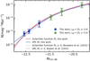 |
Fig. 13. Fit of the UV luminosity function with a DPL (blue solid line) at z = 5.6 compared to a Schechter function (red solid line). The dotted lines of respective colors are fits from the literature. The filled stars are the same as in Fig. 12. |
Parametric fitting of the UV and Lyα luminosity functions.
Both the Schechter and DPL fits represent our data well at all magnitudes. However, the reduced χ2 of the fit with DPL and α = −2.00 and ϕ* = 0.25 is lower (see Table 3) and for the bright sample (i < 25), the reduced χ2 of this fit is 2.5 times lower compared to the Schechter function fit. Since the parent catalog is complete for the bright subsample, we expect these data to be the most reliable. We conclude that the luminosity function at z ∼ 5.6 is better represented by a DPL.
4.3. Lyα luminosity function
We measured Lyα fluxes manually using the splot tool in IRAF. We proceeded in the following way: first, we interpolated the continuum flux at Lyα from the continuum levels redward of Lyα and measured the flux in the line above this level. Then, we placed the continuum level 1σ (rms of continuum measurements) above and below the average value of the continuum redward from Lyα, to estimate the uncertainties of our measurements. We also measured the ratio of continuum flux red- and blueward from Lyα for the galaxies without the emission line, but with a visible break in the continuum.
We corrected all fluxes for slit losses. Slit losses in VVDS, a survey with a nearly identical observational setup to VUDS, were extensively studied by Cassata et al. (2011) and we applied the same corrections. For the targeted galaxies, centered on the slits, the recovered flux is ∼85% and for the serendipitous objects, the median value is ∼55%.
We computed the Lyα luminosity function as described in Sect. 4.1. We present our results in Fig. 14 and Table 2. Given the detection limits for the Lyα flux in spectra, we expect our sample to be complete up to  .
.
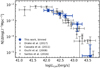 |
Fig. 14. Lyα luminosity function at the median redshift z = 5.6 (blue stars). The blue stars are results obtained from our high redshift sample, the open symbols are previous results from the literature. |
The observed bright end of the luminosity function is in good agreement with Cassata et al. (2011) (for 4.55 < z < 6.6) and Santos et al. (2016) (for LAE at z = 5.7). On the bright end, the number density decreases, but not as fast as reported from the MUSE deep fields (Drake et al. 2017) or Ouchi et al. (2008). However, the uncertainty of the MUSE data is much higher at the bright end due to the low number statistics in the brightest bins, as well as strong cosmic variance due to the small volume sampled (Moster et al. 2011).
One of the important sources of uncertainty in the Lyα luminosity function is the faint end slope. Only recently, some attempts to provide such constraints have been published, still very uncertain (Santos et al. 2016; Drake et al. 2017). Since our data do not effect enough constraints on the faint end slope, we set it to values from the literature as priors when fitting the Lyα luminosity function: α = −1.76, −2.00 (the same values, which we used for the UV luminosity function), and α = −1.69 (as used in Cassata et al. 2011). We also tested a wide range of faint end slopes from α = −1.5 to −2.3. We used uniform priors on  and ϕ* (
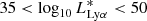 and −15 < log10ϕ* < −1) and ran MCMC minimization to find the best fit of the Lyα luminosity function.
Results are given in Table 3 and Fig. 15. As expected, uncertainties on the faint end slope lead to uncertainties on the Schechter function parameters ϕ* and M*, which were left free in the fit. As the slope α is set to steeper values, a brighter  and a lower ϕ* are obtained.
 |
Fig. 15. Lyα luminosity functions fitted with a Schechter function at redshifts 5.0 < z < 6.6. The colored solid lines are fits to our data with different faint end slopes, the gray lines are results from the literature. The filled stars are the same as in Fig. 14. |
The steep values of the faint end slope (α < −2.0) do not agree well with our data and we could not obtain a satisfactory fit with them. Recent works (Santos et al. 2016; Drake et al. 2017) suggest values of faint end slope below −2.0, but already with a slope α = −2.0, it becomes challenging to fit both the bright and faint ends in our data. A reason for the steeper faint end slope in the MUSE data lies possibly in the method used for measuring Lyα flux. Drake et al. (2017) take into account the Lyα emission in low surface brightness extended haloes. The nature of this emission remains an open question, as it may not necessarily be linked to the young stars inside the galaxy (Wisotzki et al. 2016; Leclercq et al. 2017). Given that it is more consistent with our measurements on the bright end, we conservatively chose a value of the faint end slope α = −1.69 in reporting our results, keeping in mind the uncertainty of the faint end slope constraints.
5. Star formation rate density
Using our UV and Lyα luminosity functions, we proceeded to determine the SFRD within the redshift range of our sample. To calculate the SFRD, we integrated the luminosity functions to compute the luminosity density. For Lyα emitting galaxies, we integrated from 0.04 ×  (with log
 = 43.0 from our best estimate) to log10LLyα = 44. We then transformed it to SFRD as:
![Mathematical equation: $$ \begin{aligned} \mathrm{SFRD}_{\rm Ly\alpha }[M_\odot \,\mathrm{yr}^{-1}\,\mathrm{Mpc}^{-3}] = L_{\rm Ly\alpha }[\mathrm{erg}\,\mathrm{s}^{-1}]/1.1\times 10^{42}. \end{aligned} $$](/articles/aa/full_html/2020/02/aa35400-19/aa35400-19-eq61.gif) (3)
(3)
We used the same conversion factor as Cassata et al. (2011), based on the ratio between LLyα and LHα of Brocklehurst (1971) and the conversion factor between SFR and LHα from Kennicutt (1998). We integrated the UV luminosity function from MFUV = −17.0 down to MFUV corresponding to 100 (Madau & Dickinson 2014). We used
 ![Mathematical equation: $ \kappa_{\mathrm{FUV}}=2.5 \times 10^{-10}\,[M_{\odot}\,\mathrm{yr}^{-1}\,L_{\odot}^{-1}] $](/articles/aa/full_html/2020/02/aa35400-19/aa35400-19-eq63.gif) from Madau & Dickinson (2014) to convert LFUV to SFRDFUV. For both luminosity functions, our lower integration limits correspond to the same lower SFR value enabling consistent comparison between the SFRD traced by UV and Lyα.
from Madau & Dickinson (2014) to convert LFUV to SFRDFUV. For both luminosity functions, our lower integration limits correspond to the same lower SFR value enabling consistent comparison between the SFRD traced by UV and Lyα.
We corrected SFRDFUV for dust extinction using our measurements of β slopes and IRX–β relation from Meurer et al. (1999). In Sect. 3.2, we show that UV continuum slopes steepen as we go to fainter FUV magnitudes. We used this β − MFUV relation to correct for the dust attenuation as a function of FUV magnitude when performing the integral. We obtained dust-corrected 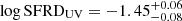 for a sample average extinction AFUV = 0.45. Results are presented in Fig. 16 and Table 3. The error bars include the uncertainties on the fit and cosmic variance. Cosmic variance is calculated using the recipe of Driver & Robotham (2010) and is equal to 5% given the geometry and population of our survey.
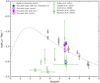 |
Fig. 16. SFRD vs. redshift. The stars are results from this work (unfilled before dust and IGM correction, filled – after). The light green points are Lyα luminosity function based measurements, the gray points are UV-based. The SFRDs from the literature are calculated from the luminosity functions using the same integration limits and conversion factors as in this work. |
We computed a UV derived SFRD of  (obtained from the best fit to the luminosity function parametrized as a DPL). We obtained the same value from the fit with the Schechter function. The increase in number density of the bright end in the case of DPL parameterization does not significantly change the estimate of the SFRD. Our result is slightly higher, by 0.2−0.3 dex, than the best fit to literature measurements as reported by Madau & Dickinson (2014) (Fig. 16), but it is in agreement with Bouwens et al. (2015a) within error bars.
The SFRD results depend evidently on our assumptions of the faint end slope value. A variation of the faint end slope by 0.2 can lead to a 0.1−0.15 dex difference on the SFRD measurement. In case of the SFRDLyα, however, our estimate remains roughly constant within error bars for slopes in a range from α = −1.5 to α = −1.85, This is because when the faint end slope steepens, the normalization density decreases acting as a compensating effect. For steeper values of α, the normalization density starts to decrease faster and the best fit of the luminosity function is forced to fall below our measurements at the bright end, which is not satisfactory. This leads to an underestimate of the contribution of bright galaxies to the SFRD. Therefore, we consider 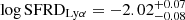 , obtained with α = −1.69, to be our best estimate of the contribution from Lyα emitting galaxies to the SFRD.
This result is in agreement within error bars with previously published results for samples selected in completely different and independent ways (Ouchi et al. 2008; Cassata et al. 2011). It differs by 0.76 dex from results obtained with MUSE observations of Hubble UltraDeep Field (Drake et al. 2017) mainly due to the very steep faint end slope used by Drake et al. (2017). Our results, however, are in broad agreement with Drake et al. (2017) when taking into account the large error bars of their measurements.
The fact that we determined both the UV and Lyα luminosity functions using the same sample of galaxies enables us to obtain a robust constraint of the ratio SFRDLyα/SFRDUV. As discussed in Hayes et al. (2011), this value is an estimate for volumetric Lyα escape fraction  . Using the same formalism, we obtained a robust estimate
 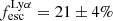 , the same as Hayes et al. (2011) estimate of
 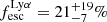 at z = 5.6 (the value from the best fit of a compilation of measurements using previous works on UV and Lyα luminosity functions).
To obtain an estimate of the total number of Lyα photons emitted within a galaxy, one has to correct for the Lyα flux absorption by the IGM. Observations of the Gunn-Peterson trough in high redshift quasars (Fan et al. 2006) indicate that more than half of the Lyα flux is absorbed by the IGM at our redshifts. The same results were obtained by Thomas et al. (2017a) from VUDS at z < 5.5. We estimated the IGM transmission of the Lyα flux directly from the spectra in our sample using the following technique: we fitted spectra with a range of SED templates leaving the IGM transmission as a free parameter. The IGM transmission was modeled using the prescription of Madau (1995), but was allowed to vary around this mean value to take into account the dispersion in transmission along different lines of sight. For the dust, we allowed the E(B − V) to vary in the range [0.0−0.1].
We found that the average Lyα transmission on our spectra is Tr(Lyα) = 0.24. We corrected the observed luminosity density LLyα by this value and thus obtained the intrinsic value of the Lyα-derived SFRD 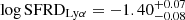 . This result is in excellent agreement with the UV-derived SFRD within error bars (see Fig. 16). Therefore, we show that using either the UV or Lyα luminosity functions, we obtain consistent estimates of the SFRD at z ∼ 5.6. It also indirectly indicates that our assumption on the low dust content of galaxies at these redshifts when computing the Lyα-derived SFRD is broadly correct. While at low redshifts, Lyα is strongly absorbed by the dust in the ISM, at high redshifts, Lyα can more efficiently escape the galaxy before entering into the IGM.
Since surveys of LAE at these redshifts use a sample selection based on the Lyα flux, we then estimated the fraction of the SFRD, which is contained in the bright end of the Lyα luminosity function. Limiting the sample to LAEs chosen to have EW > 25 Å, commonly used in the literature (Ouchi et al. 2008; Santos et al. 2016), we find that the SFRD from LAEs with EW > 25 Å includes 75% of the total SFRDUV.
Estimates of the SFRD from the UV and Lyα luminosity functions both depend on how accurately one corrects for dust, as well as for IGM absorption. The properties and the amount of dust in high redshift galaxies remain very uncertain and poorly constrained by current IR/submm data (Casey et al. 2018). Therefore, a better estimation of the amount of dust at z > 5 is necessary. Recently, Bowler et al. (2018) discovered a galaxy with a substantial dust obscuration already at z ∼ 7. If dust plays an important role in obscuring high redshift galaxies, the total SFRD at these redshifts may be even higher than derived from the UV-selected samples. Observations of the infrared to submm continuum of these galaxies are necessary to obtain more robust estimates of the total SFRD. While there are some indications of low dust content in galaxies in our sample, such as presence of galaxies with the steep β-slopes (see Sect. 3.2), it is not possible with the available data to give more robust constraints.
We note that reionization likely ended later than z ∼ 6.6. Therefore, a major fraction of Lyα emitting galaxies could be hidden at these redshifts. It has been previously shown that the fraction of LAE drops above z ∼ 6 (Stark et al. 2010; Pentericci et al. 2011; Schenker et al. 2012). This effect should be strong for our sample and contribute to a substantial reduction of the observed Lyα luminosity density. We will discuss this in detail in a forthcoming paper.
6. Summary and conclusions
In this paper, we present a sample of 49 galaxies spectroscopically confirmed at redshifts 5.0 < z < 6.6 and give simultaneously statistically robust constraints on the bright end of the Lyα and UV luminosity functions. We carefully selected galaxies using several criteria, including redshift verification, ensuring high completeness and purity. This work extends the results previously obtained to the highest redshifts probed by spectroscopic surveys (Cassata et al. 2011; Tasca et al. 2015).
We observe galaxy number densities for the UV luminosity function somewhat higher than reported in previous works (Fig. 12) but comparable to the deepest results from Bouwens et al. (2015a). The main difference between our sample and previous work is the different selection technique: in previous works (Bowler et al. 2015; Bouwens et al. 2015a) galaxies were selected based only on photometric properties, using the dropout technique. In this study, we produced a list of candidate galaxies selected from three complementary photometric techniques: photometric redshifts, the dropout technique, and the narrow band technique. These candidates were followed up with spectroscopy to establish the redshift and they needed to satisfy a rigorous set of spectroscopic and photometric criteria to make it in our final sample. This made it possible to explore larger parameter space and select galaxies with a broad range of properties, including galaxies with a strong UV-continuum, with or without Lyα in emission but also galaxies with a less pronounced continuum break and with Lyα in emission.
Our main results can be summarized as follows:
-
The brightest galaxies at z > 5 are very diverse. Some have strong Lyα emission; others do not have any Lyα emission at all. Some galaxies have steeper UV-continuum β-slopes than previously observed at this redshift (Bouwens et al. 2014), which can be seen on both spectra and photometry, while other galaxies have a flatter β-slope, indicating that some dust is present. Young dust poor galaxies are mixed with older, more dusty galaxies.
-
We observed the main sequence of galaxies in the SFR vs stellar mass plane, extending previous results (e.g., Tasca et al. 2015) to higher redshifts z > 5.0. We find no evidence for a turn-over of the main sequence at the massive end, indicating that star-formation quenching is not yet effective at these redshifts. We find that the normalization of the main sequence does not show any strong evolution above z ∼ 3.5.
-
We find that the sSFR at z > 5.0 remains similar as for 4.5 < z < 5.5. The evolution of the sSFR is, therefore, less pronounced at z > 3 and up to z ∼ 6.5 compared to the fast evolution observed at z < 3, at odds with current models (Davé et al. 2011; Sparre et al. 2015).
-
We find that the UV luminosity function at z ∼ 5.6 can be represented by either a DPL or a Schechter function, with a better fit obtained with a DPL. The UV luminosity function is comparable to other recent work (Bouwens et al. 2015a) and the integrated UV-based SFRD is 0.27 dex higher than the median reported by Madau & Dickinson (2014) at the mean redshift of z = 5.6 for our sample.
-
We find a higher number density than previous studies on the bright end of the Lyα luminosity function due to our ability to find rare bright emitters thanks to the large volume probed. We find it difficult to reconcile the high number density of bright galaxies that we find with the very steep faint end slope found by the MUSE observations (Drake et al. 2017) in a satisfactory fit with a Schechter function. Our results rather favor a shallower slope of the Lyα luminosity function of α ∼ −1.7, similar to the slope of the UV luminosity function at this redshift. We provide constraints to the SFRD associated with Lyα emitters and discuss the impact of uncertainties on α.
-
As we used the same sample for the UV and Lyα luminosity functions, we are able to compute the SFRDLyα/SFRDUV ratio in a fully consistent way. Correcting the SFRD estimated from the Lyα luminosity function for IGM absorption derived from spectral modelling of the observed spectra, we obtain very similar SFRD estimates from both the UV and Lyα luminosity functions. Limiting our analysis to LAE with EW > 25 Å, the SFRD included in these bright emitters is ∼75% of the SFRD derived from the UV luminosity function, which should be taken into account when estimating the SFRD from surveys based on LAE selection.
-
While our comparative analysis of the UV and Lyα SFRD favors low dust content in most galaxies at z ∼ 5.6, measuring the total SFRD remains dependent on accurate IGM and dust absorption corrections and some SFRD might still be missed from current UV-based surveys.
Our results, based on a sample of galaxies with confirmed spectroscopic redshifts, identify a higher number density of both UV-selected star-forming galaxies and Lyα emitters, particularly on the bright end. The SFRD derived from the corresponding luminosity functions are within the reported range of previous measurements. The steep decrease of the UV SFRD above z = 2 is confirmed up to z ∼ 6. The preferred shape of the Lyα luminosity function on the bright end as well as on the faint end still remains to be further consolidated. Future IR rest-frame surveys, for example, with ALMA and JWST, will be necessary to make further progress on constraining the SFRD at the highest redshifts.
We note that since this is a spectroscopically selected sample, we used this criterion with caution, and only in cases, where the PDF had a distinct peak or two peaks with width <1. If both peaks corresponded to redshifts compatible with zspec (for example, due to Lyman/Balmer break degeneracy), we chose the redshift with a highest probability from PDF. See also the discussion about the reliability of PDF below.
Acknowledgments
This work is supported by funding from the European Research Council Advanced Grant ERC–2010–AdG–268107–EARLY. We acknowledge the support from the grants PRIN-MIUR 2015 and ASI n.I/023/12/0 and ASI n.2018-23-HH.0. This work is based on data products made available at the CESAM data center, Laboratoire d’Astrophysique de Marseille, France.
References
- Arnouts, S., Moscardini, L., Vanzella, E., et al. 2002, MNRAS, 329, 355 [NASA ADS] [CrossRef] [Google Scholar]
- Ashby, M. L. N., Willner, S. P., Fazio, G. G., et al. 2013, ApJ, 769, 80 [NASA ADS] [CrossRef] [Google Scholar]
- Bielby, R., Hudelot, P., McCracken, H. J., et al. 2012, A&A, 545, A23 [NASA ADS] [CrossRef] [EDP Sciences] [Google Scholar]
- Bouwens, R. J., Illingworth, G. D., Oesch, P. A., et al. 2014, ApJ, 793, 115 [Google Scholar]
- Bouwens, R. J., Illingworth, G. D., Oesch, P. A., et al. 2015a, ApJ, 803, 34 [NASA ADS] [CrossRef] [Google Scholar]
- Bouwens, R. J., Illingworth, G. D., Oesch, P. A., et al. 2015b, ApJ, 811, 140 [NASA ADS] [CrossRef] [Google Scholar]
- Bouwens, R. J., Oesch, P. A., Illingworth, G. D., Ellis, R. S., & Stefanon, M. 2017, ApJ, 843, 129 [NASA ADS] [CrossRef] [Google Scholar]
- Bowler, R. A. A., Dunlop, J. S., McLure, R. J., et al. 2015, MNRAS, 452, 1817 [NASA ADS] [CrossRef] [Google Scholar]
- Bowler, R. A. A., Bourne, N., Dunlop, J. S., McLure, R. J., & McLeod, D. J. 2018, MNRAS, 481, 1631 [NASA ADS] [CrossRef] [Google Scholar]
- Brocklehurst, M. 1971, MNRAS, 153, 471 [NASA ADS] [CrossRef] [Google Scholar]
- Bruzual, G., & Charlot, S. 2003, MNRAS, 344, 1000 [NASA ADS] [CrossRef] [Google Scholar]
- Caldwell, J. A. R., McIntosh, D. H., Rix, H.-W., et al. 2008, ApJS, 174, 136 [NASA ADS] [CrossRef] [Google Scholar]
- Calzetti, D., Armus, L., Bohlin, R. C., et al. 2000, ApJ, 533, 682 [NASA ADS] [CrossRef] [Google Scholar]
- Casey, C. M., Zavala, J. A., Spilker, J., et al. 2018, ApJ, 862, 77 [NASA ADS] [CrossRef] [Google Scholar]
- Cassata, P., Le Fèvre, O., Garilli, B., et al. 2011, A&A, 525, A143 [NASA ADS] [CrossRef] [EDP Sciences] [Google Scholar]
- Castellano, M., Fontana, A., Grazian, A., et al. 2012, A&A, 540, A39 [NASA ADS] [CrossRef] [EDP Sciences] [Google Scholar]
- Chabrier, G. 2003, PASP, 115, 763 [Google Scholar]
- Ciardi, B., Ferrara, A., & White, S. D. M. 2003, MNRAS, 344, L7 [NASA ADS] [CrossRef] [Google Scholar]
- Cuillandre, J. C. J., Withington, K., Hudelot, P., et al. 2012, SPIE Conf. Ser., 8448, 84480M [Google Scholar]
- Davé, R., Oppenheimer, B. D., & Finlator, K. 2011, MNRAS, 415, 11 [NASA ADS] [CrossRef] [Google Scholar]
- Dayal, P., & Ferrara, A. 2018, Phys. Rep., 780, 1 [NASA ADS] [CrossRef] [Google Scholar]
- Dekel, A., Birnboim, Y., Engel, G., et al. 2009, Nature, 457, 451 [NASA ADS] [CrossRef] [PubMed] [Google Scholar]
- Drake, A. B., Garel, T., Wisotzki, L., et al. 2017, A&A, 608, A6 [NASA ADS] [CrossRef] [EDP Sciences] [Google Scholar]
- Driver, S. P., & Robotham, A. S. G. 2010, MNRAS, 407, 2131 [NASA ADS] [CrossRef] [Google Scholar]
- Elbaz, D., Daddi, E., Le Borgne, D., et al. 2007, A&A, 468, 33 [NASA ADS] [CrossRef] [EDP Sciences] [Google Scholar]
- Ellis, R. S., McLure, R. J., Dunlop, J. S., et al. 2013, ApJ, 763, L7 [NASA ADS] [CrossRef] [Google Scholar]
- Faisst, A. L., Capak, P., Hsieh, B. C., et al. 2016, ApJ, 821, 122 [Google Scholar]
- Fan, X., Strauss, M. A., Becker, R. H., et al. 2006, AJ, 132, 117 [NASA ADS] [CrossRef] [EDP Sciences] [Google Scholar]
- Finkelstein, S. L., Ryan, Jr., R. E., Papovich, C., et al. 2015, ApJ, 810, 71 [NASA ADS] [CrossRef] [Google Scholar]
- Garilli, B., Fumana, M., Franzetti, P., et al. 2010, PASP, 122, 827 [NASA ADS] [CrossRef] [Google Scholar]
- Grogin, N. A., Kocevski, D. D., Faber, S. M., et al. 2011, ApJS, 197, 35 [NASA ADS] [CrossRef] [Google Scholar]
- Hayes, M., Schaerer, D., Östlin, G., et al. 2011, ApJ, 730, 8 [NASA ADS] [CrossRef] [Google Scholar]
- Hinshaw, G., Larson, D., Komatsu, E., et al. 2013, ApJS, 208, 19 [NASA ADS] [CrossRef] [Google Scholar]
- Hsieh, B.-C., Wang, W.-H., Hsieh, C.-C., et al. 2012, ApJS, 203, 23 [NASA ADS] [CrossRef] [Google Scholar]
- Ilbert, O., Arnouts, S., McCracken, H. J., et al. 2006, A&A, 457, 841 [NASA ADS] [CrossRef] [EDP Sciences] [Google Scholar]
- Ishigaki, M., Kawamata, R., Ouchi, M., et al. 2018, ApJ, 854, 73 [NASA ADS] [CrossRef] [Google Scholar]
- Kashikawa, N., Shimasaku, K., Malkan, M. A., et al. 2006, ApJ, 648, 7 [NASA ADS] [CrossRef] [Google Scholar]
- Kennicutt, Jr., R. C. 1998, ApJ, 498, 541 [NASA ADS] [CrossRef] [Google Scholar]
- Koekemoer, A. M., Faber, S. M., Ferguson, H. C., et al. 2011, ApJS, 197, 36 [NASA ADS] [CrossRef] [Google Scholar]
- Le Fèvre, O., Vettolani, G., Garilli, B., et al. 2005, A&A, 439, 845 [NASA ADS] [CrossRef] [EDP Sciences] [Google Scholar]
- Le Fèvre, O., Cassata, P., Cucciati, O., et al. 2013, A&A, 559, A14 [NASA ADS] [CrossRef] [EDP Sciences] [Google Scholar]
- Le Fèvre, O., Tasca, L. A. M., Cassata, P., et al. 2015, A&A, 576, A79 [NASA ADS] [CrossRef] [EDP Sciences] [Google Scholar]
- Leclercq, F., Bacon, R., Wisotzki, L., et al. 2017, A&A, 608, A8 [NASA ADS] [CrossRef] [EDP Sciences] [Google Scholar]
- Livermore, R. C., Finkelstein, S. L., & Lotz, J. M. 2017, ApJ, 835, 113 [NASA ADS] [CrossRef] [Google Scholar]
- Lotz, J. M., Koekemoer, A., Coe, D., et al. 2017, ApJ, 837, 97 [Google Scholar]
- Madau, P. 1995, ApJ, 441, 18 [NASA ADS] [CrossRef] [Google Scholar]
- Madau, P., & Dickinson, M. 2014, ARA&A, 52, 415 [NASA ADS] [CrossRef] [Google Scholar]
- Mauduit, J. C., Lacy, M., Farrah, D., et al. 2012, PASP, 124, 714 [NASA ADS] [CrossRef] [Google Scholar]
- McCracken, H. J., Milvang-Jensen, B., Dunlop, J., et al. 2012, A&A, 544, A156 [NASA ADS] [CrossRef] [EDP Sciences] [Google Scholar]
- McGreer, I. D., Fan, X., Jiang, L., & Cai, Z. 2018, AJ, 155, 131 [NASA ADS] [CrossRef] [Google Scholar]
- McLure, R. J., Cirasuolo, M., Dunlop, J. S., Foucaud, S., & Almaini, O. 2009, MNRAS, 395, 2196 [NASA ADS] [CrossRef] [Google Scholar]
- Meurer, G. R., Heckman, T. M., & Calzetti, D. 1999, ApJ, 521, 64 [NASA ADS] [CrossRef] [Google Scholar]
- Moster, B. P., Somerville, R. S., Newman, J. A., & Rix, H.-W. 2011, ApJ, 731, 113 [Google Scholar]
- Narayanan, D., Davé, R., Johnson, B. D., et al. 2018, MNRAS, 474, 1718 [NASA ADS] [CrossRef] [Google Scholar]
- Ouchi, M., Shimasaku, K., Akiyama, M., et al. 2008, ApJS, 176, 301 [NASA ADS] [CrossRef] [Google Scholar]
- Pearson, W. J., Wang, L., Hurley, P. D., et al. 2018, A&A, 615, A146 [NASA ADS] [CrossRef] [EDP Sciences] [Google Scholar]
- Pentericci, L., Fontana, A., Vanzella, E., et al. 2011, ApJ, 743, 132 [NASA ADS] [CrossRef] [Google Scholar]
- Planck Collaboration XLVII. 2016, A&A, 596, A108 [NASA ADS] [CrossRef] [EDP Sciences] [Google Scholar]
- Planck Collaboration VI. 2018, A&A, submitted [arXiv:1807.06209] [Google Scholar]
- Prevot, M. L., Lequeux, J., Maurice, E., Prevot, L., & Rocca-Volmerange, B. 1984, A&A, 132, 389 [Google Scholar]
- Robertson, B. E., Furlanetto, S. R., Schneider, E., et al. 2013, ApJ, 768, 71 [NASA ADS] [CrossRef] [Google Scholar]
- Robertson, B. E., Ellis, R. S., Furlanetto, S. R., & Dunlop, J. S. 2015, ApJ, 802, L19 [NASA ADS] [CrossRef] [Google Scholar]
- Salmon, B., Papovich, C., Finkelstein, S. L., et al. 2015, ApJ, 799, 183 [NASA ADS] [CrossRef] [Google Scholar]
- Santini, P., Fontana, A., Castellano, M., et al. 2017, ApJ, 847, 76 [NASA ADS] [CrossRef] [Google Scholar]
- Santos, S., Sobral, D., & Matthee, J. 2016, MNRAS, 463, 1678 [NASA ADS] [CrossRef] [Google Scholar]
- Schechter, P. 1976, ApJ, 203, 297 [Google Scholar]
- Schenker, M. A., Stark, D. P., Ellis, R. S., et al. 2012, ApJ, 744, 179 [NASA ADS] [CrossRef] [Google Scholar]
- Schmidt, M. 1968, ApJ, 151, 393 [NASA ADS] [CrossRef] [Google Scholar]
- Schreiber, C., Pannella, M., Elbaz, D., et al. 2015, A&A, 575, A74 [NASA ADS] [CrossRef] [EDP Sciences] [Google Scholar]
- Scoville, N., Abraham, R. G., Aussel, H., et al. 2007, ApJS, 172, 38 [NASA ADS] [CrossRef] [Google Scholar]
- Sparre, M., Hayward, C. C., Springel, V., et al. 2015, MNRAS, 447, 3548 [Google Scholar]
- Speagle, J. S., Steinhardt, C. L., Capak, P. L., & Silverman, J. D. 2014, ApJS, 214, 15 [NASA ADS] [CrossRef] [Google Scholar]
- Spergel, D. N., Verde, L., Peiris, H. V., et al. 2003, ApJS, 148, 175 [NASA ADS] [CrossRef] [Google Scholar]
- Stark, D. P., Ellis, R. S., Bunker, A., et al. 2009, ApJ, 697, 1493 [NASA ADS] [CrossRef] [Google Scholar]
- Stark, D. P., Ellis, R. S., Chiu, K., Ouchi, M., & Bunker, A. 2010, MNRAS, 408, 1628 [NASA ADS] [CrossRef] [Google Scholar]
- Steidel, C. C., Giavalisco, M., Pettini, M., Dickinson, M., & Adelberger, K. L. 1996, ApJ, 462, L17 [NASA ADS] [CrossRef] [Google Scholar]
- Taniguchi, Y., Scoville, N. Z., Sanders, D. B., et al. 2005, J. Korean Astron. Soc., 38, 187 [NASA ADS] [CrossRef] [Google Scholar]
- Tasca, L. A. M., Le Fèvre, O., Hathi, N. P., et al. 2015, A&A, 581, A54 [NASA ADS] [CrossRef] [EDP Sciences] [Google Scholar]
- Thomas, R., Le Fèvre, O., Le Brun, V., et al. 2017a, A&A, 597, A88 [NASA ADS] [CrossRef] [EDP Sciences] [Google Scholar]
- Thomas, R., Le Fèvre, O., Scodeggio, M., et al. 2017b, A&A, 602, A35 [NASA ADS] [CrossRef] [EDP Sciences] [Google Scholar]
- Volonteri, M., & Gnedin, N. Y. 2009, ApJ, 703, 2113 [NASA ADS] [CrossRef] [Google Scholar]
- Whitaker, K. E., van Dokkum, P. G., Brammer, G., & Franx, M. 2012, ApJ, 754, L29 [NASA ADS] [CrossRef] [Google Scholar]
- Whitaker, K. E., Franx, M., Leja, J., et al. 2014, ApJ, 795, 104 [NASA ADS] [CrossRef] [MathSciNet] [Google Scholar]
- Wisotzki, L., Bacon, R., Blaizot, J., et al. 2016, A&A, 587, A98 [NASA ADS] [CrossRef] [EDP Sciences] [Google Scholar]
- Yue, B., Castellano, M., Ferrara, A., et al. 2018, ApJ, 868, 115 [NASA ADS] [CrossRef] [Google Scholar]
Appendix A: Spectra, images, and physical parameters of the whole sample
We present the physical properties of galaxies in our final sample in Table A.1, selection criteria in Table A.2, and 1D spectra and images for individual objects in the final sample in Fig. A.2. All objects are ordered by redshift. On top of 1D spectra, we plot the best SED fit to photometric points, for most of the objects coinciding with the spectra. In some cases, the SED templates may differ from the spectra due to slit losses. Some spectra have nonzero flux below Lyman limit 912 Å due to either contamination by a nearby object (see Fig. A.1) or noise at the overlap between blue and red grism.
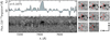 |
Fig. A.1. Spectra and 10 arcsec stamps of a galaxy with photometry contaminated by a close bright foreground object. The galaxy is pointed by red lines on the images and has an emission line seen on 1D and 2D spectra. The continuum below the emission line belongs to the bright object in the center of the images. |
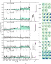 |
Fig. A.2. Spectra and 10 arcsec image stamps of the galaxies in the sample ordered by redshift. All spectra are in the rest-frame and plotted in gray. For galaxies with available photometry the photometric points are plotted in black and the best SED in light green. The PDF of photometric redshifts is plotted on the side with the real redshift marked as magenta cross. |
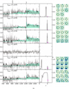 |
Fig. A.2. continued. |
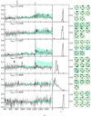 |
Fig. A.2. continued. |
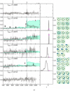 |
Fig. A.2. continued. |
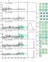 |
Fig. A.2. continued. |
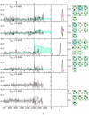 |
Fig. A.2. continued. |
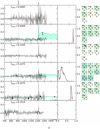 |
Fig. A.2. continued. |
 |
Fig. A.2. continued. |
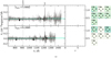 |
Fig. A.2. continued. |
Physical parameters of galaxies in our sample.
Summary of the selection criteria.
All Tables
All Figures
|
Fig. 1. Stacked spectrum of 36 galaxies with Lyα in emission. The solid line and shaded area is the observed spectrum, the dashed blue line is a Gaussian, fitted to the red wing of the emission line. The orange dotted line is the line spread function. The vertical dashed line indicates the position of Lyα line λ = 1215.7 Å. |
| In the text | |
|
Fig. 2. Redshift distribution of our sample. |
| In the text | |
|
Fig. 3. 2D spectra of VUDS galaxies with 5.0 ≤ z ≤ 6.6, ordered by redshift. The spectral range covers from 6300 to 9350 Å following the spectral region around Lyα. Lyα appears in emission or in absorption depending on spectra. |
| In the text | |
|
Fig. 4. Median stack of 36 spectra at 5.0 ≤ z ≤ 6.6 (median z ∼ 5.6) with Lyα in emission. |
| In the text | |
|
Fig. 5. Median stack of 11 spectra at 5.0 ≤ z ≤ 6.6 (median z ∼ 5.6) with Lyα in absorption. |
| In the text | |
|
Fig. 6. β-slope vs. FUV-magnitudes of our sample. Gray circles indicate the individual measurements for the galaxies with most reliable photometry, and gray crosses for the remaining ones. Blue circles are biweight means in bins of 0.7 mag size. The straight blue line is the linear fit to the biweight mean values. The colored crosses are values from Bouwens et al. (2014) and Castellano et al. (2012) at different redshifts. |
| In the text | |
|
Fig. 7. Spectra of UV bright galaxies with flat and steep UV-continuum slopes (id = 528295041 and id = 520180097 at z = 5.487 and 5.1378, respectively). The rest-frame spectra are plotted in gray and the best SED template in light green. The solid blue line shows our fit to the continuum on spectra. |
| In the text | |
|
Fig. 8. SFR–M* diagram of our sample. The solid blue line is the fit to our data, representing the main sequence of star-forming galaxies at these redshifts. The dotted cyan, orange, and green lines are extrapolations of the main sequence at our median redshift from Speagle et al. (2014), Schreiber et al. (2015), Pearson et al. (2018). Filled circles are galaxies with reliable photometry and open circles are galaxies with possible contamination from bright nearby objects. The magenta diamond is the AGN identified in our sample. The gray diamonds are estimations of SFRs from the FUV magnitudes using IRX–β relation. |
| In the text | |
|
Fig. 9. Main sequence of VUDS galaxies at different redshifts. The colored squares show the median SFR in mass bins from Tasca et al. (2015). The black circles are median SFRs from this work at 5.5 < z < 6.6. |
| In the text | |
|
Fig. 10. Redshift evolution of the sSFR. Results of various observations and numerical simulations are shown. The magenta star shows the result of this work, an extension of Tasca et al. (2015) work (light blue stars). The solid line shows the fit to the previous results from VUDS (Tasca et al. 2015), the shaded area and the dashed line shows the results, coming from the observations of EW(Hα) in COSMOS (Faisst et al. 2016). |
| In the text | |
|
Fig. 11. SSR as a function of i magnitude and the corrections applied to TSR at magnitudes i > 25, below the completeness limits. |
| In the text | |
|
Fig. 12. UV luminosity function at the median redshift z = 5.6. The blue stars are UV luminosity function estimations drawn from the bright i < 25 sample, the green stars are from the faint sample with completeness correction as described in Sect. 4.1. The black open symbols are UV luminosity function from the literature at z ∼ 5 and the gray ones at z ∼ 6. |
| In the text | |
|
Fig. 13. Fit of the UV luminosity function with a DPL (blue solid line) at z = 5.6 compared to a Schechter function (red solid line). The dotted lines of respective colors are fits from the literature. The filled stars are the same as in Fig. 12. |
| In the text | |
|
Fig. 14. Lyα luminosity function at the median redshift z = 5.6 (blue stars). The blue stars are results obtained from our high redshift sample, the open symbols are previous results from the literature. |
| In the text | |
|
Fig. 15. Lyα luminosity functions fitted with a Schechter function at redshifts 5.0 < z < 6.6. The colored solid lines are fits to our data with different faint end slopes, the gray lines are results from the literature. The filled stars are the same as in Fig. 14. |
| In the text | |
|
Fig. 16. SFRD vs. redshift. The stars are results from this work (unfilled before dust and IGM correction, filled – after). The light green points are Lyα luminosity function based measurements, the gray points are UV-based. The SFRDs from the literature are calculated from the luminosity functions using the same integration limits and conversion factors as in this work. |
| In the text | |
|
Fig. A.1. Spectra and 10 arcsec stamps of a galaxy with photometry contaminated by a close bright foreground object. The galaxy is pointed by red lines on the images and has an emission line seen on 1D and 2D spectra. The continuum below the emission line belongs to the bright object in the center of the images. |
| In the text | |
|
Fig. A.2. Spectra and 10 arcsec image stamps of the galaxies in the sample ordered by redshift. All spectra are in the rest-frame and plotted in gray. For galaxies with available photometry the photometric points are plotted in black and the best SED in light green. The PDF of photometric redshifts is plotted on the side with the real redshift marked as magenta cross. |
| In the text | |
|
Fig. A.2. continued. |
| In the text | |
|
Fig. A.2. continued. |
| In the text | |
|
Fig. A.2. continued. |
| In the text | |
|
Fig. A.2. continued. |
| In the text | |
|
Fig. A.2. continued. |
| In the text | |
|
Fig. A.2. continued. |
| In the text | |
|
Fig. A.2. continued. |
| In the text | |
|
Fig. A.2. continued. |
| In the text | |
Current usage metrics show cumulative count of Article Views (full-text article views including HTML views, PDF and ePub downloads, according to the available data) and Abstracts Views on Vision4Press platform.
Data correspond to usage on the plateform after 2015. The current usage metrics is available 48-96 hours after online publication and is updated daily on week days.
Initial download of the metrics may take a while.