| Issue |
A&A
Volume 524, December 2010
|
|
|---|---|---|
| Article Number | A46 | |
| Number of page(s) | 14 | |
| Section | Planets and planetary systems | |
| DOI | https://doi.org/10.1051/0004-6361/201015464 | |
| Published online | 23 November 2010 | |
Jupiter’s stratospheric hydrocarbons and temperatures after the July 2009 impact from VLT infrared spectroscopy
1
Atmospheric, Oceanic & Planetary Physics, Department of
PhysicsUniversity of Oxford, Clarendon Laboratory,
Parks Road,
Oxford
OX1 3PU,
UK
e-mail: This email address is being protected from spambots. You need JavaScript enabled to view it.
2
Jet Propulsion Laboratory, California Institute of Technology,
4800 Oak Grove
Drive, Pasadena,
CA, 91109, USA
3
University of California, Berkeley, Astronomy Dept., 601 Campbell Hall,
Berkeley, CA
94720-3411,
USA
4
Institut UTINAM, CNRS-UMR 6213, Observatoire de Besançon,
Université de Franche-Comté, Besançon, France
Received: 23 July 2010
Accepted: 27 August 2010
Abstract
Aims. Thermal infrared imaging and spectroscopy of the July 19, 2009 Jupiter impact site has been used to identify unique features of the physical and chemical atmospheric response to this unexpected collision.
Methods. Images and high-resolution spectra of methane, ethane and acetylene emission (7−13 μm) from the 2009 impact site were obtained by the Very Large Telescope (VLT) mid-infrared camera/spectrometer instrument, VISIR. An optimal estimation retrieval algorithm was used to determine the atmospheric temperatures and hydrocarbon distribution in the month following the impact.
Results. Ethane spectra at 12.25 μm could not be explained by a rise in temperature alone. Ethane was enhanced by 1.7−3.2 times the background abundance on July 26, implying production as the result of shock chemistry in a high C/O ratio environment, favouring an asteroidal origin for the 2009 impactor. Small enhancements in acetylene emission were also observed over the impact site. However, no excess methane emission was found over the impact longitude, either with broadband 7.9-μm imaging 21 h after the impact, or with center-to-limb scans of strong and weak methane lines between 7.9 and 8.1 μm in the ensuing days, indicating either extremely rapid cooling in the initial stages, or an absence of heating in the upper stratosphere (p < 10 mbar) due to the near-horizontal orientation of the impact. Models of 12.3-μm spectra are consistent with a ≈ 3 K rise in the lower stratosphere (p > 10 mbar), though this solution is highly dependent on the spectral properties of stratospheric debris. The enhanced ethane emission was localised over the impact streak, and was diluted in the ensuing weeks by redistribution of heated gases by zonal flow and mixing with the unperturbed jovian air.
Conclusions. The different thermal energy deposition profiles, in addition to the highly reducing (C/O > 1) environment and shallow impactor angle, suggest that (a) the 2009 plume and shock-fronts did not reach the sub-microbar altitudes of the Shoemaker-Levy 9 plumes; and (b) models of a cometary impact are not directly applicable to the unique impact circumstances of July 2009.
Key words: planets and satellites: atmospheres / atmospheric effects / planets and satellites: composition / planets and satellites: individual: Jupiter
© ESO, 2010
1. Introduction
The July 19, 2009 impact of an unidentified object with Jupiter (Sánchez-Lavega et al. 2010) is expected to have deposited significant quantities of thermal energy into the jovian stratosphere, driving unique shock-chemistry in the impact region. Models of the comet Shoemaker Levy 9 impacts in 1994 (SL9, see Harrington et al. 2004, and references therein) predict two sources of atmospheric heating: (a) kinetic energy in the heated entry channel from the incoming bolide, being disrupted and vaporised as it fell to its terminal depth; and (b) heating from the compression shock wave as the ballistic plume of material re-entered the atmosphere (Crawford 1996; Mac Low 1996; Deming & Harrington 2001). The material in the plume was a complex mixture of reprocessed material from the impactor, the unique chemical products from the shock heating of the jovian air and entrained jovian gases from the deeper troposphere (Lellouch 1996; Zahnle 1996). Excess thermal energy in the upper stratosphere was then radiated away with an approximate 1−2 day timescale (Orton et al. 1995) as the atmosphere returned to its unperturbed state.
However, Fletcher et al. (2010) demonstrated that the energy deposition from the 2009 impact was markedly different from the SL9 observations. Infrared spectroscopy from IRSHELL in 1994 (Bézard 1997; Bézard et al. 1997; Griffith et al. 1997) demonstrated that compressional heating from the collapsing plume deposited excess energy in the 5−500 μbar region, at the lower boundary of the shock. The upper stratospheric heating caused enhanced emission from the strongest CH4 lines in the ν4 vibrational band near 7.7 μm, but was absent from the weaker lines probing the lower stratosphere. This enhancement produced a strong 7.85-μm signature in IRTF/MIRAC2 imaging of the SL9 impacts (Orton et al. 1995). The temperature profiles deduced by Bézard (1997) indicated that temperature enhancements could not exceed 20 K at 1 mbar or 10 K at 10 mbar 24 h after impact. Conversely, broad-band 8−13 μm and 17−25 μm spectra of the 2009 impact from Gemini/T-ReCS (Fletcher et al. 2010) were inverted to show that no temperature perturbations were detected in the upper stratosphere, but a lower stratospheric warming of 3.5 ± 2.0 K at 10−30 mbar was observed five days after the impact.
Imaging observations at 7.9 and 12.3-μm sensitive to stratospheric temperatures and hydrocarbons.
In this paper we provide additional evidence for differences in energy deposition between the two impacts as a strong indication that the physical models of the SL9 bolide, plume and shock phases may not be directly applicable to the 2009 impact. Furthermore, we show that enhancements in hydrocarbon abundances at the impact site point to a very different composition for the 2009 impactor compared to SL9. In Sect. 2 we present the results of imaging at 7.9 and 12.3 μm in the month following the 2009 impact. Section 3 compares stratospheric temperature retrievals from CH4 emission in 8.0-μm spectra of the impact latitude obtained on July 26, 2009 and August 12, 2009, and the magnitude of upper stratospheric perturbations permitted by the data. Sections 4 and 5 compare models of ethane and acetylene emission over the impact site near 12.3 μm and 13.3 μm, respectively. The implications of the lack of stratospheric temperature enhancements and the elevated hydrocarbon abundances are discussed in Sect. 6.
2. Thermal imaging of the 2009 impact site
The first hint of differences between the 2009 and 1994 impacts came from thermal infrared imaging of the stratospheric temperature field. Imaging of the SL9 impacts from a thermal array camera, MIRAC2 (Orton et al. 1995; Friedson et al. 1995) demonstrated that 7.85 and 12.2-μm fluxes rose substantially during the R impact and plume phases, and left residual signatures that were detectable for some time afterwards (see also Conrath 1996, and references therein). This analysis of stratospheric temperatures in 2009 uses a successor to MIRAC2 mounted on the same telescope, NASA’s Infrared Telescope Facility (IRTF). The 7.9- and 12.3-μm filters are normally sensitive to stratospheric CH4 and C2H6 emission in the 0.1−20 mbar and 0.4−40 mbar regions, respectively (Fletcher et al. 2009b). If the circumstances of the 2009 impact were the same as SL9 then we would expect (a) to see thermal emission from these wavelengths in the first ≈ 48 h after the 2009 impact; and (b) that this emission would diminish over the ensuing days.
2.1. Observations
Sánchez-Lavega et al. (2010) used visible observations to show that the impact occurred between 07:40 and 14:02 UT on July 19, 2009 on the jovian nightside, creating an impact “core” or “streak” at a latitude of 55.1 ± 0.5°S (planetocentric), and System III longitude of 304.5 ± 0.5°W. Images at 7.9 and 12.3 μm sensitive to the stratospheric temperature field were obtained on several dates between July 20 and August 16, shown in Table 1. The first images from the NASA Infrared Telescope Facility (IRTF) MIRSI instrument (Mid Infrared Spectrometer and Imager, Deutsch et al. 2003) on July 20, 2009, were obtained 21−27 h after the impact occurred. With a 3-m primary mirror, the IRTF provided a diffraction-limited spatial resolution of approximately 0.65′′ ( ≈ 2000 km) at 7.9 μm, sufficient to spatially resolve the 4800 × 2500 km debris field (Sánchez-Lavega et al. 2010). Subsequent imaging was obtained with the Michelle facility mid-infrared camera/spectrometer (De Buizer & Fisher 2005) on Gemini-North and the Very Large Telescope (VLT) mid-infrared camera/spectrometer (VISIR, Lagage et al. 2004), featuring 8.1-m and 8.2-m primary mirrors, respectively. These larger telescopes provided diffraction-limited spatial resolutions as high as 0.25′′ (720 km) at 7.9 μm on nights of excellent seeing.
Images in multiple filters (7−25 μm) from all three observatories were reduced, geometrically registered, cylindrically reprojected and absolutely calibrated using the techniques developed in Fletcher et al. (2009b). Table 1 focusses solely on the 7.9- and 12.3-μm observations, but full details of the IRTF/MIRSI images are described by Orton et al. (2010) and the Gemini-N/Michelle images by de Pater et al. (2010). A subset of these observations are compared in Figs. 1 and 2.
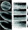 |
Fig. 1 Images of CH4 emission from Jupiter’s stratosphere (0.1−20 mbar, approximately) as described in Table 1. No perturbation from the impact (either the impact streak or crescent) is detected above the background noise and thermal wave activity. Panel a) shows an IRTF/MIRSI image from July 20, with a white arrow indicating the impact longitude. Panels b) and c) show a VLT/VISIR image from July 26, stretched to enhance contrast in panel c). Panels d)−g) are cylindrical reprojections of brightness temperature on four dates (UT times and instruments given in each panel). Any perturbation due to the impact would be expected at 55°S (planetocentric latitude) and 304.5°W (System III). All images were obtained in 7.9-μm filters, with the exception of the 7.7-μm filter on Michelle (July 22). |
2.2. Non-detection in CH4 images
Unlike the residual high-altitude thermal energy following the SL9 impacts, Fig. 1(a) shows that no perturbations of the stratospheric temperatures are evident 21−27 h after the 2009 impact. The cylindrical map of the IRTF/MIRSI data in Fig. 1(d) indicates that thermal variations smaller than approximately 1 K would be overwhelmed by (i) random error on the individual IRTF/MIRSI images and (ii) small-scale stratospheric perturbations related to dynamics and thermal wave activity. Gemini/Michelle high-resolution imaging at 7.7 μm (panel (e)) confirms the absence of stratospheric perturbations 72 h later. Finally, imaging from VLT/VISIR in panel (b) (and stretched to enhance contrasts in panel (c)) clearly demonstrates the presence of longitudinal thermal wave activity in a warm band at 50−54°S (planetocentric) and wave structures in a band poleward of 63°S, possibly associated with the edge of Jupiter’s south polar vortex. The VLT/VISIR data in Fig. 1(f, g), acquired on July 26 (one week after impact) and August 16 (one month later), shows no evidence for perturbations over the impact site. In contrast, Hubble Space Telescope imaging on August 8 (Hammel et al. 2010) showed the continuing presence of stratospheric particulates at this latitude, extending between 320 and 290° System III longitude.
Low resolution spectra of the impact site on July 24 in the 8−13 μm region (Fletcher et al. 2010) showed substantial enhancements in radiance due to the presence of stratospheric ammonia and particulate emission, interpreted as broad emission features of silicate material in the dark debris field. However, the radiance enhancement decreased to zero at the shortest wavelengths (8.0 μm), consistent with the images presented in Fig. 1. We conclude that the stratospheric particulates and ammonia (still present on July 26) had no effect on the upper-stratospheric thermal field sounded by the CH4 imaging, either by heating or cooling the overlying stratosphere. The implications of this observation are discussed in Sect. 6.3.
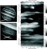 |
Fig. 2 Images of the Jupiter impact site obtained at 12.3 μm, sensitive to both upper tropospheric temperatures (note the fine-scale structure in panel a)) and emission from stratospheric C2H6. Panels a) and b) show the reduced images from IRTF/MIRSI and VLT/VISIR, respectively, with white arrows indicating the impact streak. These are cylindrically reprojected in panels c)−f) for several dates, and show that the excess emission was undetectable above the noise on August 16 (which had the poorest seeing of all the dates sampled). The broad circular artefact and dark region in the lower right of panel d), and the striations in panel e), are problems associated with striping in the VLT/VISIR images and proximity to the planetary limb. Stripes were not completely removed by the median filtering algorithm employed in the reduction. All images were obtained in 12.3-μm filters. |
2.3. Enhanced emission in C2H6 images
Unlike the 7.9-μm imaging, the impact region is clearly detected in 12.3-μm imaging presented in Fig. 2. The 12.3-μm filter is sensitive to both ethane emission in the lower stratosphere and to the collision-induced H2 continuum in the upper troposphere (note the presence of fine structure in the MIRSI image on July 20 – panel (a) – which is typical of the temperature field perturbed by tropospheric dynamics). Furthermore, structure associated with the impact streak is clearly visible in high-resolution VLT/VISIR imaging on July 24 and 26, the latter of which is shown by a white arrow in Fig. 2(b). This enhanced emission was impossible to detect above the background noise by August 16 (panel (f)), although the seeing quality was noticeably poorer on the latter date.
Given the broad spectral range covered by the 12.3-μm filter (approximately 1 μm), it is impossible to distinguish between (a) a rise in upper tropospheric temperature, raising the continuum emission; (b) warm stratospheric particulates, which also contribute to the continuum; and (c) enhanced emission from stratospheric ethane lines. However, the morphology of the 12.3-μm emission is different from images in the 8.8−11.6 μm range obtained on the same dates (e.g., Fig. 2 of de Pater et al. 2010). Instead of the well-separated impact crescent observed at these wavelengths, which is believed to be due to emission from silicate material in the dark debris (Fletcher et al. 2010), the 12.3-μm emission appears to be localised in the impact streak or “core”. The absence of the crescent from the images in Fig. 2 supports the suggestion that the silicate emission feature (peaking at 10.0 μm) contributes negligible opacity to the 12.3-μm region (Fletcher et al. 2010). We can tentatively rule out stratospheric silicate emission as contributing to the 12.3-μm images, but the degeneracy between temperatures and ethane remains problematic. We shall return to this problem with high resolution VLT/VISIR spectra in Sect. 4.
Sequence for the spectral observations from VLT/VISIR.
3. Non-detection in 8.0-μm spectroscopy
In 1994, Bézard et al. (1997) used high-spectral resolution observations to detect strong CH4 enhancements near 8.1-μm from the SL9 K and L impact sites 23 and 11 h after impact, respectively. Unfortunately, high resolution (R = 3200) spectra of the 7.9−8.1 μm region were not obtained until seven days after the 2009 impact, some time after the stratosphere should have cooled. Nevertheless, with the impact debris still present in visible images (Hammel et al. 2010), we conducted a systematic search for perturbations to the stratospheric temperatures at this latitude.
3.1. VISIR observations
Two sets of 7.9−8.1-μm spectra (R = 3200) were obtained by VLT/VISIR on July 26 and August 12, 2009, 7 and 24 days after the impact, respectively. Details of the observational sequence for both dates can be found in Table 2. A slit 32.3′′ long and 0.4′′ wide was orientated east-west, perpendicular to Jupiter’s central meridian, and centered on the latitude of the impact. A broad N-band filter (centered at the peak of the 10-μm emission) was used to identify the impact debris and place the slit at its center. Each spectrum consisted of three pairs of chop-nodded images (six files), which were processed using a combination of the ESO pipeline (via its front-end interface, GASGANO version 2.3.01), with spectral extraction and calibration performed via custom-made IDL software.
Wavelength calibration was performed by the ESO pipeline (Smette & Vanzi 2007) using off-source telluric spectral lines (from one half of the chopping cycle). The half-cycle frame was collapsed to form a one-dimensional telluric spectrum, which was then cross-correlated with a model for the atmospheric emission in this particular mode. This was used to assign wavelengths to each pixel in the dispersion direction. For each of the six files, a single differenced image (i.e. the on-source position of the chopper minus the off-source position, detecting the jovian flux on top of the telluric background) was generated, with bad pixels detected in the half-cycle frames and removed by interpolation over neighbouring pixels. The three nodded pairs were then combined (by shifting and adding using offsets computed for the on-source frames) to form the nodded 2D spectral image. This procedure was repeated for both the jovian spectra and spectra of a Cohen standard star (HD 200914) (Cohen et al. 1999) for flux calibration.
Long-slit VISIR spectra suffer from an optical distortion, which is known analytically and was corrected following the instructions in Smette & Vanzi (2007). The correct pixel values were then calculated by interpolation of the source pixel values (Pantin, pers. commun.). The spectral image was absolutely calibrated by dividing each target spectrum by the stellar spectrum and multiplying by the Cohen spectral model (Cohen et al. 1999) for that star (HD 200914). The stellar spectrum was extracted by summing the measured flux at each wavelength over all pixels with values above a certain threshold. Flux losses from the star due to the narrow width of the slit were estimated as follows: (i) acquisition imaging of the star was modelled with a convolution of an Airy function (with a Bessel correction) to represent diffraction and a Gaussian to represent seeing; (ii) the ratio of the flux lost to the flux retained in the narrow slit was used to scale the stellar spectrum. This resulted in calibrated radiance values close to those expected for Jupiter.
The final step before analysis was the assignment of latitudes, longitudes and emission angles to each position along the 32.3′′ slit. As a maximum chopping amplitude of 25′′ was used in these observations, some of the negative beam obscured the planet and was omitted from subsequent analysis. Jupiter’s limb, visible in acquisition images in the broad 10.0 μm filter, was used to deduce the latitude (54°S) and emission angle for each pixel, and the rotation of Jupiter between the final acquisition image and the time of the spectral observation (Table 2) was used to calculate longitudes.
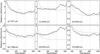 |
Fig. 3 Six examples of the variation of radiance (black dots) from west (left) to east (right) for wavelengths sensitive to CH4 emission obtained by VLT/VISIR on July 26. These radiance curves were obtained in the medium resolution (R = 3200) mode between 7.9 and 8.1 μm. The vertical dashed line is the location of the central meridian. The two dotted lines delimit the extent of the impact debris field as seen at other wavelengths, and show the absence of any thermal signature due to the impact throughout the 7.9−8.1 μm range. The smooth grey line is a model of the expected center-to-limb variation of the radiance, calculated using Cassini/CIRS T(p) profiles for this latitude, but no attempt has been made to fit the observed data. Contrasts between east and west are believed to be caused by longitudinal thermal wave activity visible in Fig. 1. The full spectrum is shown in Fig. 4. |
3.2. Center-to-limb curves
Figure 3 shows a subset of six east-west radiance scans at a particular wavelength in the July 26 dataset (i.e. the radiance values for each pixel along the length of the slit). For a completely homogeneous latitude circle, we would expect the radiance to depend solely on emission angle (higher angles probe higher, warmer stratospheric altitudes), and estimates of the center-to-limb profiles (solid grey curves) were calculated using temperature profiles derived from Cassini observations in 2000 (Fletcher et al. 2009a). However, given the longitudinal variability observed in Fig. 1, we can see that the measured radiance deviates substantially from the smooth center-to-limb curves, particularly in Figs. 3(c) and (d). These contrasts are believed to be caused by the longitudinal thermal wave activity visible in the CH4 imaging in Fig. 1. No attempt has been made to fit the grey curves to the measured data, so the close correspondence of Cassini-derived radiances with the calibrated VISIR results indicates a lack of stratospheric temperature variation during the intervening decade.
The expected location of the 2009 impact, as calculated from the N-band acquisition imaging minutes before (Table 2), is indicated by two vertical dotted lines in Fig. 3. Spectral observations at 11.6 μm (to be presented in a forthcoming publication), taken 5 minutes after the 8.0 μm spectra as part of the same template without moving the slit, showed NH3 emission at precisely the expected location. We conclude that material within the streak and crescent of the 2009 impact, comprising silicate dust and stratospheric ammonia at warm lower stratospheric temperatures, has negligible effect on the 7.9−8.1 μm spectra seven days after the impact.
3.3. Stratospheric temperature retrievals
An optimal estimation retrieval algorithm, Nemesis (Irwin et al. 2008), was used to derive the stratospheric temperature field at the impact latitude for both the July 26 and the August 12 datasets. The reference atmosphere (profiles of temperature and molecular abundances) and sources of line data were described in full by Fletcher et al. (2010). Absorption coefficients (k) for each species were used to generate k-distributions (ranking the coefficients in order of strength within a particular spectral interval) at the R = 3200 spectral resolution of the VISIR spectrometer. The tropospheric temperature structure was fixed to that derived by Cassini in 2000 (Fletcher et al. 2009a), and the temperature field at altitudes higher than the 100-mbar level was allowed to vary to fit the spectrum.
An example of the spectral fit to longitude 300°W from the July 26 data is given in Fig. 4, and this quality is typical of the 180 positions along the slit used to determine the temperature cross section. The rate of change of radiance as we vary the temperature profile (the functional derivative, or weighting function) is shown in Fig. 5. Summing over all wavelengths, the functional derivative peaks at 5.7 mbar, with a FWHM extending between 1.3 and 20.5 mbar. However, Fig. 5 indicates that there is also some sensitivity to the 3−10 μbar level in the cores of the strongest CH4 lines. It is therefore likely that we would have some sensitivity to upper stratospheric perturbations (similar to those observed during SL9 by Bézard et al. 1997) if any were present on July 26.
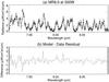 |
Fig. 4 Comparison between measured spectra – circular points with error bars – and a fitted model (solid line) on July 26 at the impact longitude (approximately 300°W). Panel b) shows the residual between the measurements and the model. The high quality of this fit is typical of all points along the VISIR slit (i.e. sampling a range of longitudes) on both dates. |
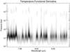 |
Fig. 5 Functional derivative between 7.9 and 8.1 μm (the rate of change of upwelling radiance with the temperature field) calculated for the T(p) profile at the impact latitude and longitude. The functional derivative has been normalised, so that the darkest regions contribute the most to the radiance. VISIR spectra exhibit some sensitivity to temperatures in the 3−10 μbar region. |
The stratospheric temperature cross sections for the impact latitude at 54°S on July 26 and August 12 are compared in Fig. 6. The impact longitude was only just visible on August 12, as it set on the eastern limb. Contrasts from east to west are believed to be caused by zonal thermal wave activity visible in the CH4 imaging in Fig. 1. However, the 17-day separation between these observations prevents characterisation of the waves from these data. On July 26 the region between 285−305°W appears to be cooler by ≈1 K at 2−3 mbar than other longitudes. However, formal retrieval errors on the absolute temperatures are on the order of 3 K at this altitude, so this slight cooling trend is not significant. This is reinforced by the absence of notable perturbations in the center-to-limb curves in Fig. 3.
However, Gemini/T-ReCS observations suggested a lower stratospheric temperature rise of 3.5 ± 2.0 K in the 10−30 mbar region on July 24 (Fletcher et al. 2010). To test the sensitivity of the VISIR spectra to such a temperature enhancement, and to high-altitude temperature perturbations such as those observed in the aftermath of SL9 (Bézard 1997), we used Gaussian perturbations to the best-fitting T(p) profile at 304°W on July 26. These temperature perturbations ranged from 1 to 40 K, and were applied at pressures from 50 mbar to 1 μbar. Uncertainty on the VISIR spectra was estimated to be 1.8 μW/cm2/sr/μm, representative of the range of east-west radiance contrasts observed along the VISIR slit. The surfaces of χ2 are shown in Fig. 7, and indicate that the maximum temperature perturbation that would go undetected within a 3σ confidence (χ2 = 9) is 3 K at 6−10 mbar. In all likelihood, such a temperature perturbation would have been detected in these spectra, suggesting either (a) a cooling of the 3.5 K enhancement at 10−30 mbar detected by T-ReCS on July 24; (b) a redistribution of the heated gases in the intervening two days (compare the impact debris field in Figs. 1, 2) or (c) an inaccurate thermal retrieval from the T-ReCS spectra due to the uncertain effects of particulate emission from the debris on July 24.
Figure 7 also demonstrates the decreasing sensitivity of the 7.9−8.1 μm spectra with altitude – for example, temperature perturbations of around 10−15 K are permitted in the 10−100 μbar region within a 3σ confidence limit. A similar decrease in sensitivity was reported by Conrath (1996) in their review of thermal measurements after SL9. But although these high-altitude temperature enhancements affect only the cores of strong CH4 lines, it is important to note that no discrete perturbations were observed at the impact longitude for any wavelength in the 7.9−8.1 μm range, both weak and strong CH4 lines alike (Fig. 3). This absence of a thermal signature will be discussed in Sect. 6.
4. Enhanced ethane emission at 12.3 μm
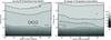 |
Fig. 6 Stratospheric temperatures retrieved from 7.9−8.1 μm spectra on July 26 (left) and August 12 (right) for the mean latitude of the impact debris (54°S). Contours are spaced every 5 K, darker shades indicate cooler temperatures. Typical errors on the stratospheric temperature are 2.7 K at 10 mbar and 3.5 K at 1 mbar. |
Low-resolution spectroscopy in the 12−13 μm region from Gemini/T-ReCS (see Fig. 2 of Fletcher et al. 2010) on July 24 demonstrated that radiances were enhanced over the impact streak but not the impact crescent. Imaging in Fig. 2 confirms that only the streak is visible at 12.3 μm. Crucially, the peak of the C2H6 emission (the ν9 band at 12.2 μm) was just as enhanced as the surrounding continuum, leading Fletcher et al. (2010) to interpret this as a rise in the lower stratospheric temperature over the impact streak. High-resolution cross-dispersed echelle spectroscopy of the impact on July 26 from VLT/VISIR also demonstrated excess emission near 12.25 μm compared to identical observations on August 13.
4.1. VISIR observations
Echelle spectroscopy of the impact site was obtained by VLT/VISIR on July 26 and August 13 2009, 7 and 25 days after the impact, respectively (Table 2). The echelle spectra require a shorter slit length (4.1′′) than the medium resolution spectra discussed in Sect. 3, so no spatial detail could be extracted. Four orders of the echelle spectra provided useful observations of the impact latitude, and here we focus on ethane emission in the 12.236−12.262 μm range. The data reduction process was identical to that described in Sect. 3.1, with the following exceptions – no optical distortion corrections were necessary, and no geometrical registration was performed in longitude-space. Instead, we used acquisition imaging to check that the slit, aligned east-west parallel to the equator, was placed at the correct latitude (53.5°S) and covered the impact longitude (304.5°W) on both dates (see Fig. 8). Radiometric errors were estimated from the standard deviation of the radiance at each wavelength along the 4.1′′ slit length.
4.2. Ethane and temperature retrievals
Using the stratospheric temperature profile retrieved in Sect. 3 as an a priori, we varied both the stratospheric T(p) and C2H6 mole fraction to reproduce the measured radiance in Fig. 9. Model fits to the two datasets are shown as solid (July 26) and dotted (August 13) black lines. Unlike the stated resolution of R = 25000 at 10.0 μm (Smette & Vanzi 2007), we found that k-distributions had to be calculated at R = 35000 at 12.25 μm to reproduce the spectra reliably. Even so, some small-scale oscillations observed in the residual between the models and data (lower panel, Fig. 9) are due to imperfect characterisation of the spectral resolution and small offsets in the wavelength calibration. Nevertheless, Fig. 9 indicates that both the ethane lines and the surrounding continuum were enhanced on July 26 compared to August 13.
The functional derivatives (rate of change of radiance with ethane abundance) in Fig. 11(a) indicate that this spectral range is sensitive to ethane variations at pressures between 0.02 and 40 mbar, permitting the retrieval of vertical profiles of C2H6 and T(p). Several different techniques were used to model the data. Firstly, we could not reproduce the data by varying the temperature profile alone. However, equally successful fits were obtained if we (a) varied both T(p) and C2H6 at the same time; and (b) if we varied C2H6 alone; thus the data does not distinguish between these two scenarios. Fig. 10 shows the outcome of the two scenarios: panels (a)−(e) show the temperature and ethane profiles required to fit the spectra when both are varied, and panels (f)−(h) show that higher C2H6 mole fractions are required when the temperature is fixed at the August 13 values. If the temperature is allowed to vary (a 2.7 ± 1.7 K rise peaking at 3 mbar), then we require a 5.0 ± 3.5 ppm ethane abundance increase centered at 0.3 mbar (Fig. 10(d)), or equivalently an increase of 2.1 ± 0.4 times the background ethane abundance centered at 6 mbar (Fig. 10(e)). Alternatively, if we fix the stratospheric temperatures to the August 13 values, then we need a larger increase of 9.8 ± 4.5 ppm centered on 0.3 mbar (Fig. 10(g)), or equivalently a 2.8 ± 0.4 times enhancement over the background at 6 mbar (Fig. 10(h)). Finally, the inclusion of aerosol opacity in the spectral models had negligible effect on the retrieved profiles, consistent with the large separation between the 12.25-μm emission and the 10-μm peak of silicate emission observed in the Gemini-S/T-ReCS observations.
In summary, the enhanced 12.25-μm emission can be explained by both (a) temperature enhancements consistent with the interpretation of Gemini-S/T-ReCS observations on July 24 (Fletcher et al. 2010); and (b) ethane enhancements over the impact location. Given that a stratospheric temperature enhancement of 2.7 ± 1.7 K is statistically permitted by the 7.9−8.1 μm spectroscopy discussed earlier (Fig. 7), it is plausible that both mechanisms contribute to the enhanced emission here. However, the absence of an 8.0-μm signature suggests that this temperature enhancement is actually at higher pressures than those implied by the C2H6-only retrievals (see Sect. 6.1), and a full explanation for the enhanced C2H6 emission will require hydrodynamic modelling of the 2009 shock circumstances.
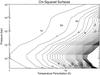 |
Fig. 7 Chi-squared surfaces for the addition of temperature perturbations to the best-fitting T(p) profile at 304°W on July 26. Temperature perturbations were modelled as Gaussian functions, with peak amplitudes between 1 and 40 K. The 1σ, 2σ and 3σ surfaces are labelled, showing the decreasing sensitivity to high altitude temperature perturbations. |
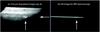 |
Fig. 8 Acquisition images of Jupiter between 07:30 and 07:40 UT on July 26 2009, just prior to echelle spectroscopy of the impact site from VLT/VISIR. White arrows show the location of the impact feature. Panel a) shows the appearance of Jupiter at 10.0 μm and the bright impact debris field (silicate and ammonia emission) in the image center). Panel b) shows that this bright point is also centrally located in the slit, and was in the center of the frame for echelle spectroscopy. |
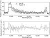 |
Fig. 9 Upper panel: comparison of the data (dots for July 26, diamonds for August 13) with spectral models (solid black line for July 26, dotted black line for August 13), showing the increased C2H6 emission on July 26. The data are an average over the 4.1′′-long slit for the cross-dispersed echelle mode of VLT/VISIR. Lower panel: residual between the data and the model for July 26 (solid black line) and August 13 (dotted black line). Models were calculated for the C2H6-only case, fixing T(p) to the August 13 values. Note that the vertical scales for a) and b) differ from one another. |
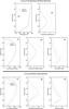 |
Fig. 10 Profiles of temperature and ethane derived from models of VLT/VISIR 12.25 μm spectroscopy of the impact site. Two different techniques for fitting the data were attempted. In the upper panels we fit the data by varying T(p) (a)−b)) and the C2H6 abundances simultaneously (c)−e)). In the lower panels we fit the data by varying C2H6 alone (f)−h)). In all cases, the solid lines are results for July 26, the dashed lines are results for August 13. The dotted lines show the formal retrieval error on the vertical profiles, though these are omitted from panels a, c and f for clarity. An enhancement of ethane is required in both scenarios. |
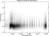 |
Fig. 11 Functional derivatives (rate of chance of radiance with variations of the gaseous abundance at each pressure level) for ethane and acetylene, in the spectral ranges covered by VLT/VISIR spectroscopy of the impact location. These plots show the altitude-sensitivity of each spectrum. The functional derivatives have been normalised to unity, with the darkest colours showing the location of maximum sensitivity. |
5. Acetylene emission at 13.3 μm
The discovery of enhanced ethane emission over the impact site prompted the search for additional hydrocarbon emission, specifically acetylene (C2H2). The zeroth order of the echelle spectroscopy described in Sect. 4.1 and Table 2 covered two C2H2 emission lines at 13.3534 and 13.3697 μm at R = 35000. However, absolute calibration of this spectrum proved particularly problematic due to the presence of a telluric absorption feature centered at 13.362 μm, right between the two jovian emission lines. The low signal to noise on the stellar calibrator in this echelle order prevented determination of the absolute radiance, so we compare line-to-continuum ratios in Fig. 12. The continuum is assumed to be the mean of the uncalibrated flux either side of the emission feature. However, the continuum may have changed between the August 13 and July 26 observations as they had done for the ethane spectra in Fig. 9.
Figure 12(a) appears to show an enhanced emission on July 26 over August 13 for the strongest of the two lines. Conversely, the enhancement observed for the weaker line in Fig. 12(b) is within the estimated error on the spectrum. Furthermore, if we calculate the expected line-to-continuum ratio by scaling the Cassini/CIRS derived C2H2 profiles of Nixon et al. (2007), we find that we need different abundances to fit each of the lines: the strongest line suggests an increased abundance by a factor of 2−3 on July 26, but the weaker line doesn’t show any increase at all. When we calculate the functional derivative (Fig. 11(b), the rate of change of the radiance with respect to C2H2), we find that the stronger line is sensitive to a greater range of altitudes (10 μbar to 20 mbar) than the weaker line (10−1000 μbar only), which suggests that either a temperature perturbation or an acetylene increase in the 1−20 mbar region is responsible for the enhanced emission at 13.3697 μm. In the absence of an absolute calibration, we cannot draw quantitative conclusions from these acetylene lines, other than stating that an increase in C2H2 emission from the 1−20 mbar region was tentatively detected over the impact location.
6. Discussion
The phenomena discussed above – the absence of upper stratospheric temperature perturbations, the possibility of heating in the lower stratosphere and the elevated abundance of ethane – demonstrate that the 2009 impact was substantially different from the collisions of the icy comet SL9. Thermal perturbations to CH4 emission were not observed, either with imaging 21 h after the impact or with high-resolution spectroscopy in the ensuing seven days. Enhancements in C2H6 and C2H2 emission were detected over the impact streak, and persisted for at least 7 days following the impact. The lack of a 7.9-μm signature favours enhanced abundances of hydrocarbons to explain these observations, rather than enhanced temperatures. However, this is inconsistent with Gemini-S/T-ReCS spectra which showed uniform radiance enhancements across the 12−13 μm range (Fletcher et al. 2010), which cannot be explained by C2H6 alone. These results raise several questions, which we discuss below.
6.1. Stratospheric cooling
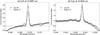 |
Fig. 12 Observations of two C2H2 lines from VLT/VISIR on July 26 (dots) and August 13 (diamonds). As absolute calibration proved difficult for these spectra, the plots are expressed as a line-to-continuum ratio, with the continuum defined by a mean of the uncalibrated flux either side of the emission features. The “dip” of the continuum is an artefact of poorly-corrected telluric absorption. Models of the expected ratio, based on scaling the C2H2 profiles of Nixon et al. (2007), are shown as dotted lines for comparison. The same models were used for panels a) and b), indicating the difficulty in determining a unique profile of C2H2 from this dataset. |
Although both the broad-band 8−13 μm T-ReCS spectra on July 24 and the 12.25-μm VISIR spectra on July 26 are consistent with a ≈ 3 K temperature enhancement in the stratosphere, this is not a unique solution, given the uncertain optical properties of the particulate dust over the impact site. The T-ReCS sensitivity to 8.0-μm (where no flux enhancement was observed) restricted the temperature perturbation to the 10−30 mbar region (Fletcher et al. 2010), whereas the VISIR spectra at 12.25 μm (i.e. without sensitivity to the 8.0-μm emission) permits the temperature enhancement to be higher up, in the 1−10 mbar region. Unfortunately, the different resolutions of the VISIR 7.9−8.1 μm spectra and the 12.25-μm spectra prevent simultaneous retrievals from both datasets, but such a retrieval would likely limit the stratospheric temperature rise to deeper levels (p > 10 mbar). Taken together, the thermal infrared spectra suggest small rises in lower stratospheric temperature (≈3 K at p > 10 mbar) which were detectable on July 24 and July 26 but had dissipated by August 13 (i.e. cooling by at least 0.15 K/day). If such a cooling trend was linear (which is extremely unlikely), then the lower stratosphere over the impact streak may have been ≈4 K warmer than the surroundings following the impact bolide and plume phases. Large temperature enhancements in the 5−500 μbar region, such as those observed following the SL9 impacts at the G, K and L sites (Bézard 1997) are not required to reproduce the 2009 data.
In their review of the available thermal measurements of the SL9 fragments, Conrath (1996) indicated that temperature perturbations of around 3−4 K above the 10-mbar pressure level were consistent with the data, and that similar perturbations in the 10−100 mbar region were feasible in the first 2−3 days following the events (e.g., Fig. 10 of Conrath 1996). They suggested that the sources of such heating could be downward penetration of heating from the fallen plumes, or buoyant adiabatic upwelling from the deeper atmosphere (see the discussion in Orton et al. 2010). Similar mechanisms could explain the lower stratospheric heating (p > 10 mbar) of the 2009 impact.
A minimum cooling rate of 0.15 K/day in the 10−100 mbar region is significantly larger than the nominal rate of radiative cooling (a 2−3 year timescale at these pressures, Bézard 1997; Conrath et al. 1990). Additional radiative cooling from the silicate debris in the 9−11 μm and 17−20 μm regions and stratospheric NH3 at 10.0 μm are likely to contribute, but we also note that significant horizontal redistribution of energy and material occurred in the week following the impact, mixing and diluting the warmer gases with unperturbed regions (Fig. 2). Estimates of the balance between excess heating from the dark silicates (solar absorption mainly at visible wavelengths) and enhanced cooling from thermal emission are extremely sensitive to (a) the mineralogical make-up; (b) the particle size distribution; and (c) the presumed altitude of the debris (Bézard 1997). Bézard’s calculations focussed on small (0.05 μm) particulate grains which condensed in the ascending SL9 plumes (Friedson 1998) and were deposited at high altitudes (p < 0.1 mbar). The estimated cooling rates may therefore be inappropriate for the larger (0.4−0.8 μm radius) tropospheric and stratospheric particulates observed in the 2009 impact (Hammel et al. 2010; de Pater et al. 2010; Orton et al. 2010). Nevertheless, it is likely that emission from the debris dominates the rapid cooling time scale for these impacts, as suggested for SL9 by Bézard (1997).
6.2. Hydrocarbon enhancements over the impact
Irrespective of the chosen temperature structure at the impact location, the VLT/VISIR 12.25-μm spectra suggest that ethane was elevated over the impact streak on July 26 by 1.7−3.2 times the abundance measured on August 13 at 6 mbar (or, equivalently, by 1.5−14.3 ppm at 0.3 mbar). Information on the spatiotemporal variability of ethane in the aftermath of SL9 is lacking due to the difficulties in identifying hydrocarbon emissions after the impacts (see the review by Lellouch 1996). Where enhancements were observed, they were attributed to rises in stratospheric temperature (Conrath 1996). Large ethylene enhancements were certainly seen (Griffith et al. 1997), but 9−14 μm spectra of the R impact (Sprague et al. 1994; Lellouch 1996) seemed to suggest suppressed ethane emission at 12.2 μm, possibly as a result of enhanced continuum emission from dust. This is in stark contrast with the 2009 analysis of the 12.25-μm excess flux, which requires enhanced C2H6 to explain.
The ethane enhancement has implications for the distinctive chemistry in the shocks of the 2009 impactor. Ethane is both destroyed and synthesised by impacts in both the shock-heated entry channel and the subsequent plume splashback, and much of the thermochemistry is controlled by the C/O ratio. The elevated ethane is not present in the crescent and is unlikely to have come from the impactor material itself. Instead, shock chemistry in “dry” jovian air (C/O > 1) leads to reduced products, with excess carbon being sequestered in HCN, C2H2 and other hydrocarbons (Zahnle 1996). Conversely, shock chemistry in “wet” jovian air (C/O < 1) produces oxidised products like CO and H2O from the excess oxygen (Zahnle 1996). Although the models of Zahnle (1996) are more applicable to the plume splashback phase, the shock heating of the entry channel is expected to have similar consequences for hydrocarbon chemistry. We would not expect ethane to be a major product of a collision with a water-rich body (confirmed by the SL9 observations), and indeed Fig. 16 of Zahnle (1996) indicates that ethane is only produced by shock chemistry under “dry” conditions. Furthermore, the “dry air” splashback models (Fig. 14 of Zahnle 1996) suggest that acetylene dominates in shock temperatures greater than 3000 K, whereas ethane and ethylene would be more readily produced at temperatures in the 2000−2600 K range. These sorts of temperatures could have been reached in large volumes surrounding the heated entry channel. The analysis of acetylene lines near 13.3 μm suggests that any enhancements in C2H2 were similar to those of C2H6, and we cannot conclude that either species was dominant.
Finally, slow upwelling of tropospheric air (responsible for the presence of NH3 in the stratosphere in both SL9 and the 2009 impacts, Griffith et al. 1997; Fast et al. 2002; Fletcher et al. 2010) could have raised this newly-produced ethane into the lower stratosphere. But given that the small tropospheric abundance of C2H6 (approximately 0.7 ppm at 200 mbar at 50°S, Nixon et al. 2007) is smaller than the quantities detected over the impact streak, some excess production of C2H6 must have occurred.
Applying these dry-air models to the 2009 impact, we conclude that shock chemistry along the impact streak must have occurred in an environment with a high C/O ratio in order to produce the reduced species. The 2009 impactor was oxygen-depleted (favouring the asteroidal impactor hypothesis, Orton et al. 2010) and small enough that it (a) did not penetrate as deep as the jovian water cloud and (b) did not produce a shock hot enough to favour acetylene over ethane production. On the other hand, the impactor must have been large enough for its shock front to penetrate beneath the NH3 cloud deck at 700−800 mbar (Fletcher et al. 2010; de Pater et al. 2010).
Once generated, ethane is a stable molecule in the Jovian stratosphere. Although photolysis could destroy a tiny fraction of the C2H6 to produce a small quantities of C2H2 in the days following the impact, the photochemical loss rates for C2H6 are so low that neither the ethane nor acetylene abundances would be significantly modified by photochemical processes in the days or even months following the impact (Moses, pers. comm.). As an alternative, the primary reason for the depletion of ethane by August 13 is dilution as the impact region expanded and mixed with unperturbed jovian air. Fast et al. (2010) used HIPWAC spectroscopy to report an increase above the quiescent background by a factor of 1.6 on August 11, two days before our August 13 observations. However, their C2H6 rise was not observed directly over the impact longitude, but was higher west of 310°W and lower to the east. Our August 13 VISIR spectra at 304°W were therefore sensitive to the “quiescent” region according to Fast et al. (2010). However, their ethane distribution is inconsistent with the uniform eastwards and westward spreading of material observed by Hubble (Hammel et al. 2010), and it may be more consistent with longitudinal thermal wave activity unrelated to the impact (i.e., stratospheric temperature perturbations observed in Figs. 1, 2) at the altitudes sensed by HIPWAC.
6.3. Absence of 7.9-μm emission 24 h post-impact
The absence of a thermal perturbation to 7.9-μm imaging from IRTF/MIRSI 21 h after the Wesley impact is puzzling. Using a similar instrument (MIRAC2) on the same telescope in 1994, Orton et al. (1995) detected 7.85-μm remnants from fragments E, Q1+R and L. Images at 7.93-μm from CFHT showed enhanced brightness over the G-Q-R-S and K+W complexes (Billebaud et al. 1995). The E site was indistinguishable 2.6 days after the impact at 7.85 μm (Orton et al. 1995), and Bézard (1997) summarizes that thermal perturbations over large sites decayed faster (1−2 days for K and L) than smaller sites (8−10 days for W, R and Q1, Kostiuk et al. 1996). Differences between the temperature perturbations over each fragment, the luminosity of the plumes and the sizes of the SL9 debris were attributed to (i) heterogeneity between comet fragments; (ii) different processes in each plume; or (iii) the different altitudes of the plume splash back (Bézard 1997; Bézard et al. 1997). Larger impacts were postulated to have produced more particulate material which persisted at high altitudes for longer, enhancing the cooling rate over those of the smaller impacts.
Each of the SL9 fragments described above were classified as large and intermediate impacts (class 1, 2a, 2b or 2c according to the scheme of Hammel et al. 1995). None of the class 3 impacts (B, N and Q2, smaller in extent) were reported to have signatures at 7.9 μm. However, given the large area of debris produced by the Wesley impactor, it seems unlikely that it can be compared to the smallest of the SL9 fragments. Nevertheless, excess thermal emission at 7.9-μm is not always detected for jovian impacts.
A full explanation for the absence of an observable upper stratospheric temperature enhancement will require comprehensive modelling of the 2009 impact circumstances (impact angle, size, mass, density, debris field and energy deposition profile). We know that similar plume and splashback processes occurred in 2009 and 1994, given the similarity of the debris and silicate emission distribution in the crescent (Fletcher et al. 2010), but the orientation and geometry of each collision were rather different. Indeed, the shallow angle of the 2009 impactor (70° from vertical, Sánchez-Lavega et al. 2010) resulted in (i) a near-horizontal orientation of the shock-heated entry channel and (ii) low vertical velocities of the re-impacting plume, which could have led to substantially different altitudes, orientations, shock velocities and energies for the 2009 plume and splashback. These differences in the altitudes of the shocks could be responsible for the absence of the 7.9-μm signature: either (a) a weak shock occurred at much higher altitudes than the microbar pressure levels (where radiative cooling would be much faster); or (b) the shock never reached the 1-mbar pressures sensed by 7.9-μm imaging.
In the first scenario, a sub-microbar weak shock would cause a reduced amount of heating; cooling would be more rapid; and neither IRTF nor VLT 7.9-μm data would be sensitive to the signatures of the impact. However, this is difficult to reconcile with the shock-produced debris (silicates, silicas and other dark particulates) that are known to be present in the upper troposphere and lower stratosphere soon after the impact (Hammel et al. 2010; de Pater et al. 2010; Fletcher et al. 2010). Subsidence of the debris from microbar pressures to the tropopause is extremely unlikely over such short timescales, and our observations seem to favour the second scenario.
For the second scenario, we utilise Eq. (3) of the ballistic trajectory reconstruction of Sánchez-Lavega et al. (2010) (based on the SL9 analysis of Jessup et al. 2000) to estimate the maximum height of the plume above the 100-mbar pressure level. For an ejection velocity of 7.6 ± 0.5 km s-1 and an elevation angle of 70 ± 5°, we estimate maximum altitudes of  km above the 100-mbar pressure level, at a time
  s after the ejection. Conversely, using elevation angles and ejection velocities typical of SL9, we find that the maximum plume height can be up to 2500 km (e.g., consistent with observations, Jessup et al. 2000). Taking the 100-mbar surface as a reference level, the 2009 plume rose no higher than the 1−800 μbar level, so this ballistic analysis suggests a much lower altitude for the shock-related energy deposition and chemistry. Indeed, the 2009 plume may never have left the influence of frictional drag, and particulate trajectories cannot be regarded as truly unimpeded. Given that the shock front penetrated to at least 1 bar (from enhanced NH3 over the impact streak, Fletcher et al. 2010), the shallow entry angle implies that the rising plume would have needed to travel over much greater distances to reach the microbar pressures of the SL9 shock fronts (e.g., Deming & Harrington 2001), and would have been prone to greater frictional dissipation as it travelled through the collapsing entry column (Palotai, pers. comm.).
We must also question our ability to detect the 7.9-μm signature of an impact with a shallow entry angle – kinetic energy transferred to the stratosphere by the incoming bolide would have been distributed over a wider horizontal area and smaller vertical extent compared to SL9. As a result, it would contribute less to the upwelling radiance than if the energy had been deposited over a greater vertical range. Finally, the initial cooling of the plume (over tens of minutes) could have been so rapid that no trace of a 7.9-μm signature remained by the time of the first IRTF/MIRSI observations 21−27 h later. The ultimate resolution of the absence of the 7.9-μm signature will require detailed modelling of the 2009 shock orientation, strength and altitude for rocky and icy bodies of a range of densities and sizes.
7. Conclusions
Spectroscopy of methane, ethane and acetylene emission obtained by VLT/VISIR have been analysed to study the temperature and hydrocarbon distributions over the July 2009 impact site. In addition, contextual imaging for these spectra were provided by a number of ground-based observatories. A synthesis of all the available infrared data allows us to draw the following conclusions:
-
1.
Ethane enhancement: spectra of C2H6 emission at 12.25-μm suggest that ethane was elevated on July 26 by 1.7−3.2 times the abundance measured on August 13 at 6 mbar (or, equivalently, by 1.5−14.3 ppm at 0.3 mbar). Ethane production in shock chemistry is favoured in environments with a high C/O ratio, implying that the 2009 impactor was oxygen-depleted and small enough that it (a) did not penetrate as deep as the jovian water cloud and (b) did not produce a shock hot enough to favour acetylene over ethane production. These results favour an asteroidal rather than cometary origin for the 2009 impactor.
-
2.
Hydrocarbon distribution: 12.3-μm imaging suggested that emission enhancements from C2H6 and the surrounding continuum were localised over the impact streak (and absent from the crescent, consistent with low resolution spectroscopy of the 12−13 μm region, Fletcher et al. 2010). This supports the suggestion that silicate emission from the debris has a negligible contribution to the 12.3-μm spectrum. The ethane enhancements persisted for at least 7 days following the impact, when they were first measured by VISIR spectroscopy. The primary mechanism for the return to the quiescent atmospheric state by August 13 was dilution as the impact region expanded and mixed with unperturbed jovian air.
-
3.
Upper stratospheric temperatures (p < 10 mbar): No excess methane emission from the impact longitude was observed in any of the 7.9-μm datasets – neither 21 h after the collision by IRTF/MIRSI, nor in the ensuing days from center-to-limb spectral scans by VLT/VISIR. It is likely that inhomogeneous emission from these stratospheric levels is dominated by longitudinal thermal wave activity, particularly in a warm band at 50−54°S, which may mask any signature due to the impact shocks. The elevated N-band emission from silicate dust and stratospheric NH3, which was still present in the lower stratosphere on July 26, had no heating or cooling effect on the overlying atmosphere. Finally, no perturbations were observed even in the strongest CH4 lines (sensitive to μbar pressures), so no excess thermal energy was detected in the upper stratosphere.
-
4.
Lower stratospheric temperatures (p > 10 mbar): models of VLT/VISIR 12.3-μm spectra show a degeneracy between temperature and ethane abundance. Although a C2H6 enhancement on July 26 is certainly required, the data are also consistent with a lower stratospheric temperature rise of ≈ 3 K at p > 10 mbar. This is in agreement with low-resolution spectroscopy of the 12−13 μm region by Gemini/T-ReCS on July 24 (Fletcher et al. 2010), and such a small perturbation may not have been detected (to within 3σ) in the CH4 emission spectra. It is plausible that both a small temperature enhancement and a rise in ethane are responsible for the enhanced ethane and continuum emission observed by VISIR and T-ReCS. Finally, an enhancement in acetylene emission at 13.3 μm was also consistent with increased temperature and/or C2H2 in the 1−20 mbar region. Indeed, in the aftermath of SL9, Conrath (1996) speculated that the source of such lower stratospheric heating might be downward penetration of heating from the fallen plumes, or buoyant adiabatic upwelling from the deeper atmosphere.
-
5.
Stratospheric cooling:12−13 μm data were consistent with a lower stratospheric temperature enhancement on July 24 and 26, but this had dissipated by August 13 due to redistribution of heated gases by zonal flow and dilution with unperturbed jovian air. This rate of cooling was considerably faster than typical radiative relaxation times, likely due to the enhanced emission from stratospheric silicate debris and NH3 (Bézard 1997). The efficiency of this cooling (and indeed the magnitude of the temperature perturbation retrieved from thermal infrared spectra) is highly sensitive to the composition, size distribution, spectral properties and altitude of the particulate debris.
The absence of the 7.9-μm signatures of thermal perturbations in the upper stratosphere and the possible presence of lower stratospheric heating, combined with the lower stratospheric population of NH3 and silicate debris, suggests considerable differences between the altitudes reached by the 2009 plume and splash compared to SL9. The low altitudes of the 2009 shock heating, particulate production and chemistry are due to the shallow angle of the impact (70° from vertical, Sánchez-Lavega et al. 2010) and the possible high bulk density (an asteroidal impactor, given the strongly reducing chemistry in a C > O environment). Alternatively, the cooling rate at high altitude may have been so rapid (due to a large population of currently unidentified small dust particles) that no trace of a 7.9-μm signature remained 21 h after impact. For all of these scenarios, it is clear that models of the SL9 impacts are not directly applicable to the July 2009 events, and that there are substantial modelling opportunities to answer remaining questions about the differences between the 2009 and SL9 impacts.
Acknowledgments
Fletcher was supported during this research by a Glasstone Science Fellowship at the University of Oxford. Orton carried out part of this research at the Jet Propulusion Laboratory, California Institute of Technology, under a contract with the National Aeronautics and Space Administration.
We thank E. Pantin, B. Bézard, A. Sánchez-Lavega, R. Hueso, C. Palotai, T. Greathouse and P. Irwin for their helpful comments and suggestions during the writing of this manuscript. In particular, we thank J. I. Moses for a thorough review. We wish to thank observers at the VLT, IRTF and Gemini for their rapid and effective response to the 2009 impact on Jupiter. This work was partially based on the following observations: (1) VLT/VISIR observations from UT3/Melipal collected at the European Organisation for Astronomical Research in the Southern Hemisphere, Chile, under Directors Discretionary program ID 283.C-5043. (2) MIRSI observations in program 2009A-073 obtained at the Infrared Telescope Facility, which is operated by the University of Hawaii under Cooperative Agreement no. NNX-08AE38A with the National Aeronautics and Space Administration, Science Mission Directorate, Planetary Astronomy Program. (3) MICHELLE observations obtained at the Gemini Observatory (Director Discretionary program GN-2009A-DD-7), which is operated by the Association of Universities for Research in Astronomy, Inc., under a cooperative agreement with the NSF on behalf of the Gemini partnership: the National Science Foundation (United States), the Science and Technology Facilities Council (United Kingdom), the National Research Council (Canada), CONICYT (Chile), the Australian Research Council (Australia), Ministrio da Cincia e Tecnologia (Brazil) and Ministerio de Ciencia, Tecnologa e InnovaciŮn Productiva (Argentina).
References
- Smette, A., & Vanzi, L. 2007, VLT/VISIR User Manual, vlt-man-eso-14300-3514 edn., European Southern Observatory [Google Scholar]
- Bézard, B. 1997, Planet. Space Sci., 45, 1251 [NASA ADS] [CrossRef] [Google Scholar]
- Bézard, B., Griffith, C. A., Kelly, D. M., et al. 1997, Icarus, 125, 94 [NASA ADS] [CrossRef] [Google Scholar]
- Billebaud, F., Drossart, P., Vauglin, I., et al. 1995, Geophys. Res. Lett., 22, 1777 [NASA ADS] [CrossRef] [Google Scholar]
- Cohen, M., Walker, R. G., Carter, B., et al. 1999, ApJ, 117, 1864 [Google Scholar]
- Conrath, B. J. 1996, in The Collision of Comet Shoemaker-Levy 9 and Jupiter, ed. K. S. Noll, H. A. Weaver, & P. D. Feldman, IAU Colloq., 156, 293 [Google Scholar]
- Conrath, B. J., Gierasch, P. J., & Leroy, S. S. 1990, Icarus, 83, 255 [NASA ADS] [CrossRef] [Google Scholar]
- Crawford, D. A. 1996, in The Collision of Comet Shoemaker-Levy 9 and Jupiter, ed. K. S. Noll, H. A. Weaver, & P. D. Feldman, IAU Colloq., 156, 133 [Google Scholar]
- De Buizer, J., & Fisher, R. 2005, in High Resolution Infrared Spectroscopy in Astronomy, ed. H. U. Käufl, R. Siebenmorgen, & A. Moorwood, 84 [Google Scholar]
- de Pater, I., Fletcher, L. N., Perez-Hoyos, S., et al. 2010, Icarus, 210, 722 [NASA ADS] [CrossRef] [Google Scholar]
- Deming, D., & Harrington, J. 2001, ApJ, 561, 468 [NASA ADS] [CrossRef] [Google Scholar]
- Deutsch, L. K., Hora, J. L., Adams, J. D., & Kassis, M. 2003, in Instrument Design and Performance for Optical/Infrared Ground-based Telescopes, ed. I. Masanori, & A. F. M. Moorwood, Proc. SPIE, 4841, 106 [Google Scholar]
- Fast, K., Kostiuk, T., Romani, P., et al. 2002, Icarus, 156, 485 [NASA ADS] [CrossRef] [Google Scholar]
- Fast, K., Kostiuk, T., Livengood, T., Hewagama, T., & Amen, J. 2010, in EGU General Assembly, EGU2010–14959 [Google Scholar]
- Fletcher, L. N., Orton, G. S., Teanby, N. A., & Irwin, P. G. J. 2009a, Icarus, 202, 543 [NASA ADS] [CrossRef] [Google Scholar]
- Fletcher, L. N., Orton, G. S., Yanamandra-Fisher, P., et al. 2009b, Icarus, 200, 154 [NASA ADS] [CrossRef] [Google Scholar]
- Fletcher, L. N., Orton, G. S., de Pater, I., et al. 2010, Bull. Am. Astron. Soc., 42, 1010 [NASA ADS] [Google Scholar]
- Friedson, A. J. 1998, Icarus, 131, 179 [NASA ADS] [CrossRef] [Google Scholar]
- Friedson, A. J., Hoffmann, W. F., Goguen, J. D., et al. 1995, Geophys. Res. Lett., 22, 1569 [NASA ADS] [CrossRef] [Google Scholar]
- Griffith, C. A., Bezard, B., Greathouse, T. K., et al. 1997, Icarus, 128, 275 [NASA ADS] [CrossRef] [Google Scholar]
- Hammel, H. B., Beebe, R. F., Ingersoll, A. P., et al. 1995, Science, 267, 1288 [NASA ADS] [CrossRef] [PubMed] [Google Scholar]
- Hammel, H. B., Wong, M. H., Clarke, J. T., et al. 2010, ApJ, 715, 150 [Google Scholar]
- Harrington, J., de Pater, I., Brecht, S. H., et al. 2004, Lessons from Shoemaker-Levy 9 about Jupiter and planetary impacts (New York: Cambridge Planetary Science. Cambridge Univ. Press), 159 [Google Scholar]
- Irwin, P., Teanby, N., de Kok, R., et al. 2008, J. Quant. Spectr. Radiat. Trans., 109, 1136 [NASA ADS] [CrossRef] [Google Scholar]
- Jessup, K. L., Clarke, J. T., Ballester, G. E., & Hammel, H. B. 2000, Icarus, 146, 19 [NASA ADS] [CrossRef] [Google Scholar]
- Kostiuk, T., Buhl, D., Espenak, F., et al. 1996, Icarus, 121, 431 [NASA ADS] [CrossRef] [Google Scholar]
- Lagage, P. O., Pel, J. W., Authier, M., et al. 2004, The Messenger, 117, 12 [NASA ADS] [Google Scholar]
- Lellouch, E. 1996, in The Collision of Comet Shoemaker-Levy 9 and Jupiter, ed. K. S. Noll, H. A. Weaver, & P. D. Feldman, IAU Colloq., 156, 213 [Google Scholar]
- Mac Low, M. 1996, in The Collision of Comet Shoemaker-Levy 9 and Jupiter, ed. K. S. Noll, H. A. Weaver, & P. D. Feldman, IAU Colloq., 156, 157 [Google Scholar]
- Nixon, C. A., Achterberg, R. K., Vinatier, S., et al. 2007, Icarus, submitted [Google Scholar]
- Orton, G., A’Hearn, M., Baines, K., et al. 1995, Science, 267, 1277 [NASA ADS] [CrossRef] [PubMed] [Google Scholar]
- Orton, G. S., Fletcher, L. N., Lisse, C. M., et al. 2010, Icarus, submitted [Google Scholar]
- Sánchez-Lavega, A., Wesley, A., Orton, G., et al. 2010, ApJ, 715, 155 [Google Scholar]
- Sprague, A. L., Hunten, D. M., Witteborn, F. C., et al. 1994, BAAS, 26, 1579 [NASA ADS] [Google Scholar]
- Zahnle, K. 1996, in The Collision of Comet Shoemaker-Levy 9 and Jupiter, ed. K. S. Noll, H. A. Weaver, & P. D. Feldman, IAU Colloq., 156, 183 [Google Scholar]
All Tables
Imaging observations at 7.9 and 12.3-μm sensitive to stratospheric temperatures and hydrocarbons.
All Figures
|
Fig. 1 Images of CH4 emission from Jupiter’s stratosphere (0.1−20 mbar, approximately) as described in Table 1. No perturbation from the impact (either the impact streak or crescent) is detected above the background noise and thermal wave activity. Panel a) shows an IRTF/MIRSI image from July 20, with a white arrow indicating the impact longitude. Panels b) and c) show a VLT/VISIR image from July 26, stretched to enhance contrast in panel c). Panels d)−g) are cylindrical reprojections of brightness temperature on four dates (UT times and instruments given in each panel). Any perturbation due to the impact would be expected at 55°S (planetocentric latitude) and 304.5°W (System III). All images were obtained in 7.9-μm filters, with the exception of the 7.7-μm filter on Michelle (July 22). |
| In the text | |
|
Fig. 2 Images of the Jupiter impact site obtained at 12.3 μm, sensitive to both upper tropospheric temperatures (note the fine-scale structure in panel a)) and emission from stratospheric C2H6. Panels a) and b) show the reduced images from IRTF/MIRSI and VLT/VISIR, respectively, with white arrows indicating the impact streak. These are cylindrically reprojected in panels c)−f) for several dates, and show that the excess emission was undetectable above the noise on August 16 (which had the poorest seeing of all the dates sampled). The broad circular artefact and dark region in the lower right of panel d), and the striations in panel e), are problems associated with striping in the VLT/VISIR images and proximity to the planetary limb. Stripes were not completely removed by the median filtering algorithm employed in the reduction. All images were obtained in 12.3-μm filters. |
| In the text | |
|
Fig. 3 Six examples of the variation of radiance (black dots) from west (left) to east (right) for wavelengths sensitive to CH4 emission obtained by VLT/VISIR on July 26. These radiance curves were obtained in the medium resolution (R = 3200) mode between 7.9 and 8.1 μm. The vertical dashed line is the location of the central meridian. The two dotted lines delimit the extent of the impact debris field as seen at other wavelengths, and show the absence of any thermal signature due to the impact throughout the 7.9−8.1 μm range. The smooth grey line is a model of the expected center-to-limb variation of the radiance, calculated using Cassini/CIRS T(p) profiles for this latitude, but no attempt has been made to fit the observed data. Contrasts between east and west are believed to be caused by longitudinal thermal wave activity visible in Fig. 1. The full spectrum is shown in Fig. 4. |
| In the text | |
|
Fig. 4 Comparison between measured spectra – circular points with error bars – and a fitted model (solid line) on July 26 at the impact longitude (approximately 300°W). Panel b) shows the residual between the measurements and the model. The high quality of this fit is typical of all points along the VISIR slit (i.e. sampling a range of longitudes) on both dates. |
| In the text | |
|
Fig. 5 Functional derivative between 7.9 and 8.1 μm (the rate of change of upwelling radiance with the temperature field) calculated for the T(p) profile at the impact latitude and longitude. The functional derivative has been normalised, so that the darkest regions contribute the most to the radiance. VISIR spectra exhibit some sensitivity to temperatures in the 3−10 μbar region. |
| In the text | |
|
Fig. 6 Stratospheric temperatures retrieved from 7.9−8.1 μm spectra on July 26 (left) and August 12 (right) for the mean latitude of the impact debris (54°S). Contours are spaced every 5 K, darker shades indicate cooler temperatures. Typical errors on the stratospheric temperature are 2.7 K at 10 mbar and 3.5 K at 1 mbar. |
| In the text | |
|
Fig. 7 Chi-squared surfaces for the addition of temperature perturbations to the best-fitting T(p) profile at 304°W on July 26. Temperature perturbations were modelled as Gaussian functions, with peak amplitudes between 1 and 40 K. The 1σ, 2σ and 3σ surfaces are labelled, showing the decreasing sensitivity to high altitude temperature perturbations. |
| In the text | |
|
Fig. 8 Acquisition images of Jupiter between 07:30 and 07:40 UT on July 26 2009, just prior to echelle spectroscopy of the impact site from VLT/VISIR. White arrows show the location of the impact feature. Panel a) shows the appearance of Jupiter at 10.0 μm and the bright impact debris field (silicate and ammonia emission) in the image center). Panel b) shows that this bright point is also centrally located in the slit, and was in the center of the frame for echelle spectroscopy. |
| In the text | |
|
Fig. 9 Upper panel: comparison of the data (dots for July 26, diamonds for August 13) with spectral models (solid black line for July 26, dotted black line for August 13), showing the increased C2H6 emission on July 26. The data are an average over the 4.1′′-long slit for the cross-dispersed echelle mode of VLT/VISIR. Lower panel: residual between the data and the model for July 26 (solid black line) and August 13 (dotted black line). Models were calculated for the C2H6-only case, fixing T(p) to the August 13 values. Note that the vertical scales for a) and b) differ from one another. |
| In the text | |
|
Fig. 10 Profiles of temperature and ethane derived from models of VLT/VISIR 12.25 μm spectroscopy of the impact site. Two different techniques for fitting the data were attempted. In the upper panels we fit the data by varying T(p) (a)−b)) and the C2H6 abundances simultaneously (c)−e)). In the lower panels we fit the data by varying C2H6 alone (f)−h)). In all cases, the solid lines are results for July 26, the dashed lines are results for August 13. The dotted lines show the formal retrieval error on the vertical profiles, though these are omitted from panels a, c and f for clarity. An enhancement of ethane is required in both scenarios. |
| In the text | |
|
Fig. 11 Functional derivatives (rate of chance of radiance with variations of the gaseous abundance at each pressure level) for ethane and acetylene, in the spectral ranges covered by VLT/VISIR spectroscopy of the impact location. These plots show the altitude-sensitivity of each spectrum. The functional derivatives have been normalised to unity, with the darkest colours showing the location of maximum sensitivity. |
| In the text | |
|
Fig. 12 Observations of two C2H2 lines from VLT/VISIR on July 26 (dots) and August 13 (diamonds). As absolute calibration proved difficult for these spectra, the plots are expressed as a line-to-continuum ratio, with the continuum defined by a mean of the uncalibrated flux either side of the emission features. The “dip” of the continuum is an artefact of poorly-corrected telluric absorption. Models of the expected ratio, based on scaling the C2H2 profiles of Nixon et al. (2007), are shown as dotted lines for comparison. The same models were used for panels a) and b), indicating the difficulty in determining a unique profile of C2H2 from this dataset. |
| In the text | |
Current usage metrics show cumulative count of Article Views (full-text article views including HTML views, PDF and ePub downloads, according to the available data) and Abstracts Views on Vision4Press platform.
Data correspond to usage on the plateform after 2015. The current usage metrics is available 48-96 hours after online publication and is updated daily on week days.
Initial download of the metrics may take a while.